Abstract
Plant breeders make selection decisions based on multiple traits, such as yield, plant height, flowering time, and disease resistance. A commonly used approach in multi-trait genomic selection is index selection, which assigns weights to different traits relative to their economic importance. However, classical index selection only optimizes genetic gain in the next generation, requires some experimentation to find weights that lead to desired outcomes, and has difficulty optimizing nonlinear breeding objectives. Multi-objective optimization has also been used to identify the Pareto frontier of selection decisions, which represents different trade-offs across multiple traits. We propose a new approach, which maximizes certain traits while keeping others within desirable ranges. Optimal selection decisions are made using a new version of the look-ahead selection (LAS) algorithm, which was recently proposed for single-trait genomic selection, and achieved superior performance with respect to other state-of-the-art selection methods. To demonstrate the effectiveness of the new method, a case study is developed using a realistic data set where our method is compared with conventional index selection. Results suggest that the multi-trait LAS is more effective at balancing multiple traits compared with index selection.
Keywords: multi-trait genomic selection, simulation, optimization, Genomic Prediction
GENOMIC selection (GS), which was initially proposed by Meuwissen et al. (2001), is a special form of marker assisted selection (MAS) that simultaneously estimates the effects of genome-wide markers in a training population consisting of genotyped and phenotyped individuals. Selection decisions are based on genomic estimated breeding values (GEBVs) in a breeding population, which are calculated as the sum of the estimated marker effects. The advantages of GS have been demonstrated by simulation and empirical studies (Meuwissen et al. 2001; Schaeffer 2006; Goddard 2009; Makowsky et al. 2011; Wang et al. 2018).
Previous studies have focused mainly on the development of models to improve the accuracy of GEBV prediction. Until recently, few studies have considered alternatives to truncation selection on GEBVs followed by random mating of the selected individuals. These studies have focused on selecting the parents of the next generation by defining new quantitative selection metrics (Goddard 2009; Daetwyler et al. 2015; Goiffon et al. 2017; Moeinizade et al. 2020) or jointly considering selection and mating decisions (Akdemir and Sánchez 2016; Moeinizade et al. 2019). The latter two methods are forms of mate selection (Kinghorn and Shepherd 1999) that optimize the contributions of potential parents to the next generation based on maximizing a desired breeding objective. Typically, the optimization is performed with respect to the next generation (Akdemir and Sánchez 2016; Kinghorn and Kinghorn 2016). Look-ahead mate selection (LAMS) schemes that optimize parental contributions with respect to grand-progeny (i.e., two generations in the future) have also been proposed in the context of animal breeding (Hayes et al. 1998, 2002; Shepherd and Kinghorn 1998).
Moeinizade et al. (2019) implemented a LAMS scheme—look-ahead selection (LAS)—in a stochastic simulation framework that seeks to optimize the performance of the best possible progeny in an arbitrarily defined terminal generation. This strategy was shown to outperform conventional genomic selection (Meuwissen et al. 2016), optimal haploid value selection (Daetwyler et al. 2015), and optimal population value selection (Goiffon et al. 2017) using empirical data from a population of maize inbred lines. LAS outperformed previous approaches by achieving more genetic gain and preserving more genetic diversity over the course of a simulated breeding program.
Although LAS presents a significant improvement over competing methods, it is confined to single trait genomic selection (ST-GS). Generally, the productivity of a crop variety is dependent on multiple characteristics such as yield, grain quality, and disease resistance. Hence, selection and mating decisions should be based on several different characteristics with potentially different breeding goals. Multi-trait selection poses difficulties for breeders because it often requires balancing competing breeding objectives. Four principle multi-trait genomic selection (MT-GS) strategies have been proposed in the literature: (1) tandem selection, whereby different traits are selected independently in different generations (Burgess and West 1993); (2) independent culling, whereby truncation selection is performed on multiple traits simultaneously with independent thresholds (Hazel 1943); (3) index selection, whereby multiple traits are selected at the same time by constructing an index that is a linear combination of multiple traits (Hazel and Lush 1942; Hazel 1943); and (4) mate selection, whereby multiple traits are selected at the same time by finding Pareto optimal solutions of a mate selection index (Kinghorn and Kinghorn 2016).
Tandem selection, by definition, is not capable of selecting multiple traits simultaneously, and is most useful when some traits should be selected in earlier generations than others. Independent culling does perform simultaneous selection but is very sensitive to the truncation points for the different traits. Index selection has become an important method that has been widely used for the development of superior varieties in both animal and plant breeding (Villanueva and Woolliams 1997; Jannink et al. 2000; Ivkovich and Koshy 2002; Sharma and Duveiller 2003; Long et al. 2006; Yan and Frégeau-Reid 2008). This often takes the form of truncation selection on an index constructed by integrating information on the economic values of the different traits and their phenotypic and additive genetic covariances. Brascamp (1984) provides a concise summary of different selection indices. Mate selection can consider different constraints and breeding goals for multiple traits, and evaluates these criteria in the context of a proposed set of matings. Two recent studies in plants have evaluated the use of mate selection on long-term genetic gains (Suontama et al. 2018; Cowling et al. 2019). Additionally, Akdemir and Sánchez (2016) and Akdemir et al. (2019) have developed new mate-selection methods for single- and multi-trait scenarios, respectively, with an emphasis on application to plant breeding.
An additional challenge in multi-trait selection is the definition of breeding objectives for each trait. For example, a breeder wishing to maximize grain yield might also need to maintain minimum standards for standability and disease resistance, and an acceptable range of plant heights. Kempthorne and Nordskog (1959) proposed maintaining a trait at an optimal level by weighting its squared deviations from the optimum. Wilton et al. (1968) generalized this approach to include both squares and cross products of multiple traits. Moav and Hill (1966) developed a graphical method to calculate explicitly nonlinear indices on two traits. Later, iterative solutions were developed to identify the optimal weights for a nonlinear index on an arbitrary number of traits Itoh and Yamada (1988); Pasternak and Weller (1993). However, the general solution for the weights of a nonlinear index is dependent on the population mean prior to selection and the intensity of selection (Weller et al. 1996). Therefore, the optimum selection index changes each generation and will be different from an index that maximizes gains over multiple generations.
In this paper, we propose an extension of the single-trait LAS method to multiple traits with different breeding objectives. The method maximizes a single, main trait while constraining other traits to fall within flexibly defined ranges. It retains the advantages of single-trait LAS derived from considering the impacts of selection, mating, and resource allocation decisions on the performance of individuals in the terminal generation of the breeding program.
Materials and Methods
Data sets
A dataset of 5022 maize recombinant inbred lines (RILs) from the US nested association mapping (US-NAM) (Yu et al. 2008) and intermated B73xMo17 (IBM) (Lee et al. 2002) populations was used in this study. Best linear unbiased predictors (BLUPs) for total kernel weight were taken from Yang et al. (2018). BLUPs for ear height were calculated from the phenotypic data in Kusmec et al. (2017) using a mixed model with genotype and environment as random effects. The mixed model was implemented in the R package lme4 (Bates et al. 2015).
SNPs from Kusmec et al. (2017) were thinned using PLINK v1.90b (Chang et al. 2015) using the “indep-pairwise” function with a window size of 250 kb, a step size of 50 SNPs, and a linkage disequilibrium (LD) threshold of 0.6. Thinned SNPs were imputed and phased with Beagle v4.0 (Browning and Browning 2008) using default parameters. This produced 359,826 imputed and phased SNPs. SNP effects for each phenotype were estimated using the BayesB algorithm (Meuwissen et al. 2001) implemented in GenSel4 (Fernando and Garrick 2009). Recombination rates were estimated using the genetic map for the US-NAM population (Yu et al. 2008) following the procedure outlined in Goiffon et al. (2017).
Simulation design
A total of 100 independent simulations of a 10-generation breeding program were performed using a maize data set. An initial population of 200 individuals was randomly selected from the full data set, and, in each generation, 20 individuals were selected to make 10 crosses. More details on the simulation steps are available in Goiffon et al. (2017) and Moeinizade et al. (2019).
Single-trait LAS
In this section, we review the LAS method that was recently proposed for single-trait genomic selection (Moeinizade et al. 2019). To make this algorithm more robust, we present an equivalent reformulation of this method and then discuss how this algorithm can be extended for multiple trait settings in the next section.
The single-trait LAS (ST-LAS) method anticipates the consequences of selection and mating decisions over several generations via simulation by quantitatively taking into account recombination frequencies during meiosis. The ST-LAS method has made three major contributions to the literature: (1) time management: ST-LAS is the only GS method that takes time constraints into account and is deadline sensitive; (2) mating strategy optimization: the ST-LAS method not only makes the selection decisions but also specifies how to pair the selected individuals for mating; and (3) resource allocation: this method uses a heuristic strategy to allocate more progeny to crosses between more diverse parents to increase the probability of producing high performing individuals.
The cornerstone of this method is evaluating a given selection and mating strategy by estimating the distribution of progeny GEBVs in the final generation. By simulating the GEBVs of a random sample of individuals in the final generation, a breeder can make better selection and mating decisions. This method can be formulated as the following optimization model (Moeinizade et al. 2019):
| (1) |
| (2) |
| (3) |
| (4) |
| (5) |
This optimization model has two decision variables: x, which represents the selection strategy, and y, which represents the mating strategy. Below is a detailed description of the objective as well as all variables and parameters used in this model:
fLas: The expected GEBV of the best offspring in the terminal generation.
xn: A binary decision variable that shows whether individual n is selected or not
yi,j: A binary variable that shows whether individual i is mated with individual j or not
The recombination frequency vector.
τ: The remaining number of generations ( where t is the current generation and T is the deadline generation number).
N: The number of individuals in the population.
S: The number of individuals that are to be selected out of the current population.
As demonstrated in Equation (1), the objective of the ST-LAS method is dependent on selection (x), mating (y), recombination frequencies (r), and remaining number of generations (τ). Constraint (2) states that S individuals are selected from total N individuals in the population to make S/2 crosses (assuming that S is an even number) and constraint (3) ensures that the decision variable x, is binary. Constraint (4) ensures that each selected individual is mated once. Finally, constraint (5) states that the decision variable y is binary.
In this model, evaluation of is very challenging because of the uncertainty involved due to recombination frequencies (r) and also selection (x) and mating (y) decisions over T − t generations. To deal with these challenges, a simulation optimization algorithm was designed that estimates and maximizes the LAS objective function by exploring the selection and mating solution space efficiently.
Equivalent formulation of ST-LAS
According to Moeinizade et al. (2019), the objective of ST-LAS is to maximize the expected GEBV of the best offspring in the terminal generation (Equation 1). The best offspring can be the individual with maximum expected GEBV in the final generation; however, the maximum value does not necessarily represent the whole distribution. To make the prediction more robust and reduce the influence of outliers, we present an equivalent reformulation of the ST-LAS method (Equations 6–8) where the best offspring is defined as the 100γth percentile among predicted GEBVs of individuals in the terminal generation.
| (6) |
| (7) |
| (8) |
Here, φ is a threshold value, equivalent to the previous objective fLas, which represents the expected GEBV of the best offspring in the final generation, where best is defined as the 100γth percentile of the simulated GEBV distribution. The new variables and parameters are defined as follow:
φ: The expected GEBV of the best offspring in the terminal generation.
The expected GEBV of a random progeny in the terminal generation (for trait 1 which is the only trait in the case of ST-LAS).
γ: A parameter that defines which percentile of the GEBV distribution is evaluated in the final generation.
In this model, constraint (8) states that, for a random progeny in the final generation, the probability of having an expected GEBV at least equal to the threshold value is ≥1 − γ. For example, for a random sample of 1000 progeny, if γ = 0.98, then ϕ will evaluate the GEBV of the top 2% of progeny.
Multi-trait LAS
In this section, we present a new approach for MT-GS problems to optimize the main goal of a breeding program while keeping other traits within desired ranges. This new approach, multi-trait LAS (MT-LAS), extends the ST-LAS method to multiple trait settings. It should be noted that the same resource allocation heuristic from Moeinizade et al. (2019) is applied to MT-LAS. This resource allocation strategy aims to preserve more genetic diversity by varying the number of progeny produced from each cross relative to their breeding parents genetic diversity.
Assume there exists J different traits, of which one, j = 1 (e.g., yield), should be maximized while the other traits, (e.g., plant height, ear height, etc.), should satisfy certain criteria. This problem can be formulated as an optimization model as follows:
| (9) |
| (10) |
| (11) |
This model shares the same objective and constraints (2), (3), (4), and (5) with the equivalent reformulation of ST-LAS. However, constraint (11) is a modification of constraint (8), which focuses on making sure that traits fall into desired ranges by defining a conditional probability. Below is a detailed description of all new variables and parameters: his model shares the same objective and constraints (2), (3), (4), and (5) with the equivalent reformulation of ST-LAS. However, constraint (11) is a modification of constraint (8), which focuses on making sure that traits j ∈ { 2,3,..., J } fall into desired ranges by defining a conditional probability. Below is a detailed description of all new variables and parameters:
: The expected GEBV of a random progeny in the terminal generation for trait j where
lj: The lower value for trait j.
uj: The upper value for trait j.
This model aims to maximize the expected GEBV of the top 100 (1−γ)% of offspring in the terminal generation for the trait of interest (e.g., yield) among offspring that also meet thresholds with respect to other traits (e.g., plant height, grain quality, etc.). Without loss of generality, or capture the cases when only a lower bound or upper bound should be considered. Note that when only one trait (j = 1) is considered, this formulation is equivalent to ST-LAS.
The ST-LAS optimization model was already challenging to solve, and, after adding a nonlinear and nonconvex constraint (11), the computational complexity increases significantly. To overcome this challenge, we redefine constraint (11) by converting the conditional probability on l and u to a penalty that dynamically adjusts the objective function in response to violations of the boundaries. The penalty allows violations of the boundaries that are offset by improvements in the objective function. Take, for example, the case that the decision maker wants to maximize yield while making sure that plant height does not exceed a certain value. What if we could improve yield by slightly violating the height constraint? We want the height constraint to be true, but not at the expense of losing the main objective.
The following mathematical model formulates the problem:
| (12) |
| (13) |
| (14) |
| (15) |
| (16) |
| (17) |
Here, θj is the probability that a random progeny is acceptable in the final generation with respect to trait j for and The new function is a linear combination of the expected GEBV of a random progeny for trait and the penalty of violating the desired range for traits
Here are some properties of constraints (14)–(17):
The term in Equation (15) represents the penalty for violating the upper or lower bounds for a random progeny in the terminal generation. As the magnitude of the violation increases, the penalty term increases. In the case of no violation, the penalty becomes 0.
From Equation (17), the term is the weighted sum of penalties for all traits of The weight (1 − θj) is the probability that a random progeny violates the desired range.
When all the individuals with respect to traits (e.g., height) are acceptable, θ1 = 1 and the focus will be only on the trait of interest (e.g., yield).
The sum of all weights in Equation (17) equals 1
The larger θ1, the more weight is placed on the trait of interest (e.g., yield) in selection and mating decisions.
After evaluation of the MT-LAS objective function, the next step is to optimize the model. A similar heuristic algorithm from Moeinizade et al. (2019) is used to optimize the MT-LAS model. This algorithm is defined as follows.
Algorithm 1 Heuristic for optimizing the MT-LAS model
Select S random individuals from the population
Randomly mate selected individuals
Set as list of positions to check
Set as number of positions to check
while nf ≥ 0 do
Generate as a random integer
Swap j with every unselected individual from population
for every possible swap w
if then
Reject the swap and keep j
Remove the zth position on from f
else
Accept the swap
nf = S − 1
end
end
Example with illustration
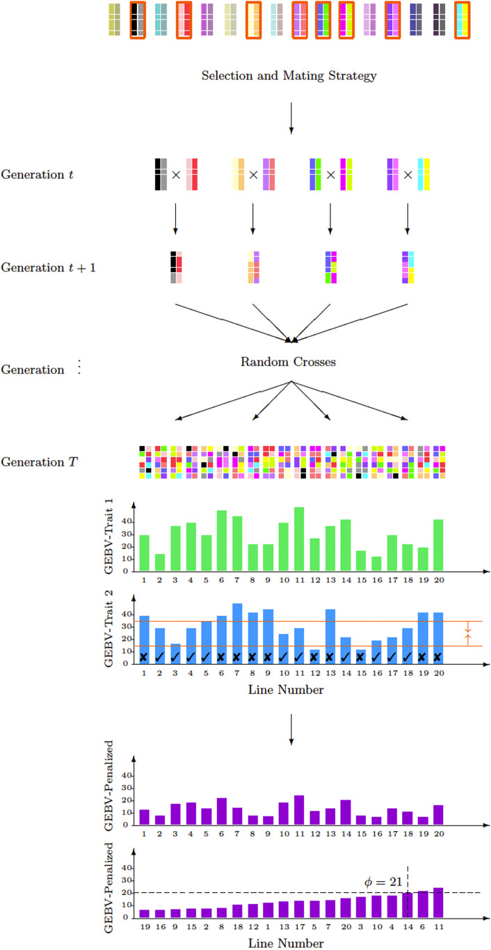
In this section, we illustrate the MT-LAS method with an example to provide a more intuitive description. Assume that the goal is maximizing yield (trait 1) while ensuring that plant height (trait 2) falls within a desired range. For a given selection and mating strategy at the current generation (t), the look-ahead stochastic simulation predicts the GEBV of individuals in the final generation (T) with respect to both traits as illustrated in Figure 1.
Figure 1.
The look-ahead simulation illustration for MT-LAS method. In this example, the population consists of 16 individuals. In generation t, eight individuals are selected from the population and mated accordingly to make four crosses. Each breeding parent produces one progeny in generation t + 1 and from generation t + 1 to T − 1 all progeny are crossed with each other in the same generation, each producing one progeny. Then, the look-ahead objective can be approximated by taking a random sample of progeny in generation T. In this example, 20 lines are produced and the GEBV of each individual with respect to traits 1 and 2 are measured and visualized with green and blue bars, respectively. Our goal is to maximize trait 1 after T − t generations while making sure that trait 2 does not exceed a certain value of u = 35 and is not <l = 15. We observe that 10 individuals among 20 are not acceptable. The progeny with acceptable values for bounded trait are distinguished with check marks. The penalized GEBVs are calculated and represented as purple bars and calculation of the objective ϕ is demonstrated for a given γ.
In this example, 20 random progeny are produced in the final generation. The GEBVs of these progeny for both traits are approximated with the look-ahead algorithm. In Figure 1, the green and blue bars represent the GEBVs for each progeny with respect to traits 1 and 2 [i.e., and , respectively]. GEBVs for plant height are constrained to fall between 15 and 35. Hence, among all progeny, lines 1, 6, 7, 8, 9, 12, 13, 15, 19, and 20 are not acceptable for plant height. These progeny are distinguished from progeny that meet the height requirements with a cross mark. Because 10 out of 20 individuals meet the height criterion, θ1 and θ2 are both 0.5. Finally, the penalty (∆) and penalized GEBVs for each progeny are calculated using Equations (15) and (17), respectively. Penalized GEBVs are plotted as the purple bars in Figure 1.
After sorting the progeny with respect to penalized GEBVs, we can calculate the objective ϕ. Let us assume γ = 0.90. The 90th percentile among 20 individuals is the third best individual and according to Figure 1, line 14 is the third best individual. Hence, we have which is the value of for line 14.
Data availability
The authors state that all data necessary for confirming the conclusions presented in the article are represented fully within the article. Data are available at figshare (DOI: 10.25380/iastate.12145752).
Results
In this section, we present a case study with real data. Without loss of generality, two traits—total kernel weight (TKW) and ear height (EHT)—are used in this case study. Our objective is to maximize TKW given a constraint on EHT.
We first present the performance of ST-LAS where the goal is to maximize TKW only. In this way, we can observe the behavior of EHT vs. TKW in the absence of any constraints on EHT. Then, we investigate truncation selection on a selection index for TKW and EHT with different choices of weights. However, this does not allow keeping a trait within a specified range. Hence, we define a penalized index by assigning a negative weight on the absolute deviations from the specified range. The penalized index is used as a benchmark against the performance of MT-LAS. Finally, we present the MT-LAS results and compare the effectiveness of MT-LAS to that of the penalized index.
ST-LAS : maximizing TKW
In this section, we investigate the behavior of EHT over 10 generations when the objective is to maximize TKW and there is no constraint on EHT. This will help provide reasonable bounds for EHT when testing the MT-LAS algorithm.
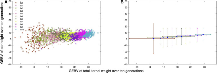
Figure 2A presents the total kernal weight and ear height GEBVs over 10 generations for a single simulation when selection is only on TKW. Over 10 generations, the mean GEBV of TKW increases from 2.78 to 40.25 with a maximum of 47.09. For EHT, the range of GEBVs changes from [−21.87,25.42] to [−1.68,14.77]. Figure 2B presents the minimum, mean, and maximum GEBVs of both traits over 10 generations averaged over 100 simulation replicates. On average, the GEBVs of EHT fall in a range of [−2.73, 16.54] in the final generation.
Figure 2.
(A) Population GEBVs of EHT vs. TKW for one simulation replicate over 10 generations when selection and mating decisions are optimized using ST-LAS algorithm with an objective of maximizing TKW. Each generation includes 200 individuals represented by stars and different colors are distinguishing between generations. The final generation has a minimum, mean, and maximum of 34.36, 40.25, 47.09 for TKW and −1.68, 7.17, 14.77 for EHT respectively. (B) Minimum, mean and maximum GEBVs of TKW and EHT over 10 generations averaged over 100 simulation replicates. Selection and mating decisions are optimized using ST-LAS algorithm with an objective of maximizing TKW. The final generation has a minimum, mean, and maximum of 33.30, 39.04, 44.51 for TKW and −2.73, 7.00, 16.54 for EHT respectively.
Index selection: maximizing TKW and EHT with assigned weights
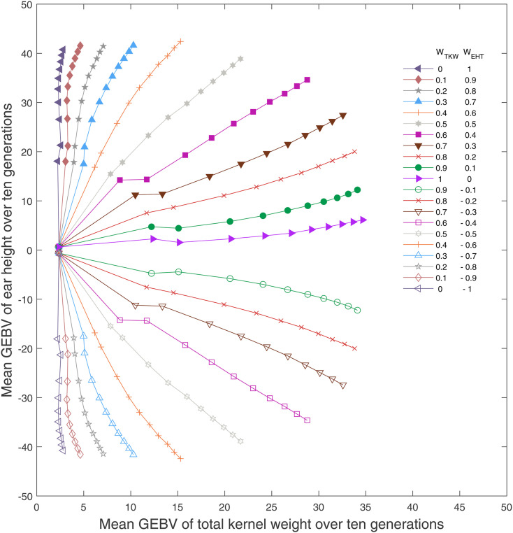
A selection index is a linear combination of traits according to some weighting scheme. Typically, truncation selection is applied to the index. Here, we construct an index for TKW and EHT where the index is the weighted sum of the GEBVs for each trait and truncation selection is applied to the index. Let WTKW and WEHT be the weights placed on the GEBVs for total kernel weight and ear height, respectively. Weights are chosen from the real numbers between −1 and 1. It should be noted that, in this scheme, we are selecting for larger values of both TKW and EHT. Placing a negative weight on a trait selects for smaller values and produces progress in the opposite direction to that under strictly positive weights. Figure 3 presents the average GEBVs over 10 generations averaged over 100 replicate simulations under index selection with varying weights, including the case where the weight on EHT is negative.
Figure 3.
Index selection considering different weights for TKW and EHT averaged over 100 simulation replicates. The mean GEBV of individuals over 10 generation are calculated given a pair of weights for two traits. The absolute values of the weights add up to one. Each curve demonstrates the mean GEBV of individuals (represented by markers) over 10 generations for assigned weights.
As expected, increased weight for EHT (positive or negative) negatively impacts the efficiency of selection for TKW. The mean GEBVs for both traits change in the direction of their assigned weights over time, indicating the lack of strong genetic correlations between TKW and EHT. The highest mean GEBV for TKW (34.67) is achieved by selection solely on TKW Table 1 provides the minimum, mean, and maximum GEBVs for TKW in the final generation under the different choices for weights. It should be noted that the maximum GEBV for TKW achieved after 10 generations of selection is less than that achieved using ST-LAS (36.05 vs. 44.51). This considerable impact on response is due to the fact that the LAS focuses on maximizing the expected GEBV of the best offspring in the terminal generation, considering uncertainty in recombination in each generation, whereas truncation selection on GEBVs focuses on maximizing the genetic gain in the next generation. Additionally, LAS selects pairs of individuals as a group and recognizes the importance of mating.
Table 1. Summary statistics of population GEBV values in generation 10 averaged over 100 replicate simulations for TKW using conventional genomic selection with different weights (index selection).
| WTKW | WEHT | Min | Mean | Max |
|---|---|---|---|---|
| 0 | ±1 | 0.22 | 2.81 | 5.41 |
| 0.1 | ±0.9 | 1.86 | 4.63 | 7.53 |
| 0.2 | ±0.8 | 4.23 | 7.08 | 9.86 |
| 0.3 | ±0.7 | 7.21 | 10.28 | 13.3 |
| 0.4 | ±0.6 | 12.07 | 15.30 | 18.43 |
| 0.5 | ±0.5 | 18.53 | 21.68 | 24.69 |
| 0.6 | ±0.4 | 25.86 | 28.77 | 31.6 |
| 0.7 | ±0.3 | 30.21 | 32.57 | 34.85 |
| 0.8 | ±0.2 | 32.00 | 33.81 | 35.49 |
| 0.9 | ±0.1 | 32.69 | 34.11 | 35.48 |
| 1 | 0 | 33.29 | 34.67 | 36.05 |
These results are based on simulations in Figure 3
Penalized index selection: maximizing TKW with a constraint on EHT
In this section, we reformulate the index selection to be able to specify a desired range for the secondary trait. This enables a direct comparison to the MT-LAS method. After applying ST-LAS to TKW, the GEBVs for EHT in the final generation fell between −2.73 and 16.54. We subsequently investigated three cases where EHT is constrained to fall outside this range of variation. The three cases are as follows:
• Case 1:
• Case 2:
• Case 3:
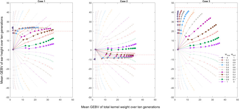
Similar to the use of a quadratic index to approach an optimum phenotype (Kempthorne and Nordskog 1959; Wilton et al. 1968), we define an index that penalizes the absolute deviations from a desired range. The constructed index is formulated as . Weights are chosen from the real numbers between 0 and 1, constrained to sum to unity. Figure 4 presents the average GEBVs over 10 generations averaged over 100 replicate simulations under penalized index selection for three different cases. These results are compared against the index selection without penalization from Figure 3. We observe that the nonpenalized index selection cannot satisfy the EHT criterion. As expected, over multiple generations of selection the GEBV of TKW increases and the penalty term accommodates keeping EHT within the specified range. For case 1 and case 2, the EHT criterion is satisfied when WEHT ≥ 0.3. However, for case 3, the criterion cannot be satisfied even with the penalized index selection because the bound represents an extreme case. The behavior of case 3 is very similar to the index selection without penalization.
Figure 4.
Penalized index selection considering different weights for TKW and EHT averaged over 100 simulation replicates for three different cases. Each curve demonstrates the mean GEBV of individuals (represented by markers) over 10 generations for assigned weights. The transparent curves in the background present the index selection results without penalization and the red dashed lines are the decision boundaries.
MT-LAS: maximizing TKW with a constraint on EHT
The MT-LAS method aims to maximize genetic gain in a target trait while ensuring that one or more secondary traits fall within specified boundaries. Here, we maximize TKW subject to constraints on EHT for three different cases.
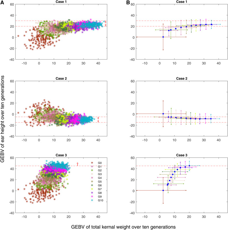
Population GEBVs over 10 generations for one simulation replicate are presented in Figure 5A, and the average of 100 simulation replicates are presented in Figure 5B. For cases 1 and 2, the GEBVs for EHT of ∼90% of the individuals in the final generation fall within the specified boundaries. For case 3, only a lower bound on EHT GEBV was specified. This bound represents an extreme case where index selection is unable to achieve the lower bound even when selecting solely on EHT. However, MT-LAS is able to exceed the bound, with ∼50% of the population falling into the acceptable range.
Figure 5.
(A) GEBVs of individuals over 10 generations for one simulation replicate. Optimal selection and mating decisions were made using the MT-LAS method in all three cases. Generations are distinguished with different colors. Over multiple generations of selection, the GEBV of TKW increases and the GEBV of EHT falls within the desired range. The red dashed lines are the decision boundaries and the arrows demonstrate the direction for which the condition is satisfied. (B) Minimum, mean and maximum GEBVs over 10 generations averaged over 100 simulation replicates. The blue markers in the middle of cross marks are the mean GEBVs and the end of the cross marks represent minimum and maximum GEBVs.
Comparison: performance of MT-LAS against penalized index selection
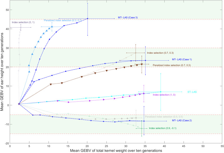
Figure 6 compares the performance of MT-LAS with the results of nonpenalized and penalized index selection using weights that produced results satisfying the desired ranges for three cases. We also show that ST-LAS for TKW exceeds the performance of truncation selection on TKW alone For both cases 1 and 2, MT-LAS is able to produce populations that surpass the performance of the comparable index selection scenarios with respect to TKW, and also keep almost all individuals within the specified boundaries for EHT. For case 3, the highest EHT achieved by index selection with or without penalization cannot satisfy the desired range criterion. However, MT-LAS not only achieves the expected EHT, but also improves the TKW considerably.
Figure 6.
Comparison of MT-LAS, ST-LAS and index selection methods. The mean GEBVs of population over 10 generations are averaged over 100 simulation replicates and represented for two traits. Furthermore, the minimum and maximum GEBVs in the final generation are demonstrated using the cross marks. The green bar specifies the boundaries.
Overall, using MT-LAS with optimization of selection and mating decisions, and a soft penalty on EHT, improves the response. It should be noted that the distributions of look-ahead methods are quite different from index selection. As shown in Figure 6 the look-ahead methods achieve wider distributions in the terminal generation.
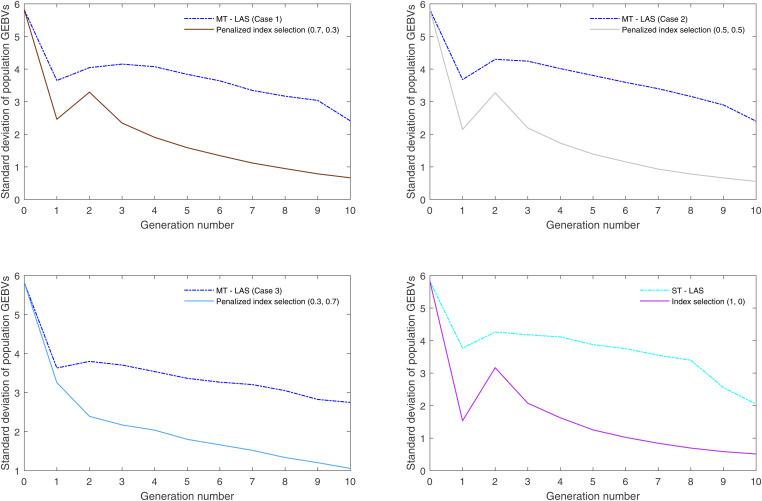
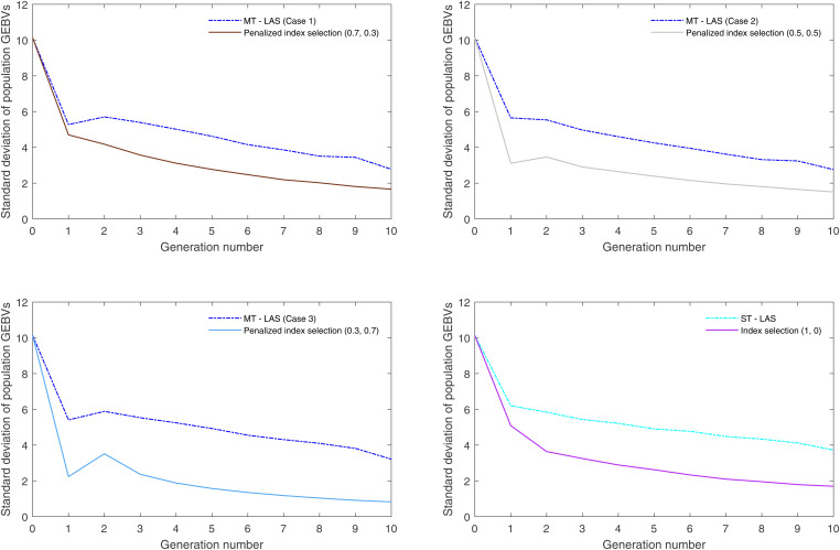
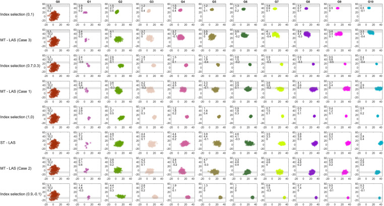
Figures 7 and 8 display the SD of population GEBVs over 10 generations for 100 simulation replicates and compare the performance of MT-LAS/ST-LAS with index selection. As expected, look-ahead methods maintain more genetic variance than index selection, indicating that there is greater room for population improvement after 10 generations. Furthermore, the genetic correlations between two traits are presented over time for one simulation replicate, which indicate the lack of strong correlation between TKW and EHT (see Figure 9 in Appendix).
Figure 7.
SD of total kernel weight GEBVs over time averaged for 100 simulation replicates.
Figure 8.
SD of ear height GEBVs over time averaged for 100 simulation replicates.
Figure 9.
Comparison of the population performance for MT-LAS, ST-LAS, and index selection methods over 10 generations for one simulation replicate. The gray bars specify boundaries. Each box has three numbers including SD of population GEBVs for trait 1 and trait 2 as well as the correlation between two traits from top to bottom, respectively.
Discussion
The production of a crop variety depends on multiple characteristics, such as grain quality, yield, and drought resistance, which are subject to different breeding objectives. In this study, we proposed a new multi-trait selection approach using genomic information that maximizes genetic gain with respect to a focal trait while controlling the variation in multiple secondary traits.
To demonstrate the effectiveness of the proposed method, we conducted a case study using real data where MT-LAS is compared with index selection with varying weights. In this case study, the goal was to maximize TKW while constraining EHT. Three different cases with varying bounds were investigated, and the results suggested that MT-LAS was more effective at balancing multiple traits than index selection.
Fundamentally, the MT-LAS algorithm surpassed conventional index selection because of four reasons. The first reason is the satisfiability of this method. MT-LAS automatically and dynamically balances multiple traits and is able to optimize selection and mating decisions in a way that satisfies the constraints for bounded traits, while simultaneously maximizing the main trait of interest in the terminal generation. For two of our three scenarios, the penalized index was able to satisfy the constraints on the bounded trait, but at the cost of reduced performance in the maximized trait. Moreover, with index selection, it may not be possible to achieve some values for the bounded traits without mate selection. For example, in case 3, we investigate the performance of MT-LAS with a lower bound of 45, which is not reached with either nonpenalized or penalized index selection (Figures 3 and 4).
The second advantage of MT-LAS is its dynamic adjustability. The MT-LAS method places more emphasis on feasibility requirements (having individuals that meet the thresholds for the bounded traits) when most of the individuals are not predicted to fall within the bounds for the bounded traits in the terminal generation. On the other hand, this algorithm focuses on the main trait when most of the individuals become acceptable for the bounded trait. Overall, selection and mating decisions are dynamically adjusted in every generation by making a trade off between optimizing the main goal and reaching the desired range for the bounded traits.
A third benefit of MT-LAS is its interpretability. By defining the weights in terms of bounds on the desired values of the trait, MT-LAS provides an intuitive description of the breeding objective on the original measurement scale.
A fourth benefit of MT-LAS is its time-awareness. As opposed to classical index selection, which maximizes genetic merit in the next generation, MT-LAS maximizes genetic merit in an arbitrary terminal generation. This is similar to work on look-ahead mate selection in animal breeding (Hayes et al. 1998; Shepherd and Kinghorn 1998; Hayes et al. 2002), where the quantity to be maximized is the genetic merit of grand-progeny. Additionally, this shift alleviates the difficulties posed by the dependence of classical nonlinear indices on the current generation mean and intensity of selection, which can cause such an index to be nonoptimal over multiple generations (Weller et al. 1996).
The main contribution of MT-LAS is constraints (14), (16), and (17), which allow the algorithm to adjust the objective function dynamically according to the progress of the current population. Future research is needed to more fully characterize the MT-LAS algorithm and address the limitations of this study. First, the current paper considers only two traits, although the model is formulated for J traits. Further simulations to explore the behavior of the algorithm when constraining more than one trait are desirable. Second, the hyper-parameter γ plays a crucial role in identifying the optimal selection and mating decisions. In this study, we selected γ after experimenting with several values. Future work is needed to design systematic methods for optimizing this parameter. Third, the objective of the look-ahead selection relates to the final generation and future research can focus on designing new selection methods that also consider intermediate generations in the objective. Finally, we based our simulations on a single data set from a single crop organism. Further simulations considering more diverse populations are necessary to demonstrate the general applicability of MT-LAS.
Acknowledgments
Any opinions, findings, conclusions, or recommendations expressed in this publication are those of the author(s) and do not necessarily reflect the view of the United States Department of Agriculture (USDA). This work is supported by Agriculture and Food Research Initiative grant no. 2017-67007-26175/accession no. 1011702 from the USDA National Institute of Food and Agriculture. This work is also supported by the Plant Sciences Institute’s Faculty Scholars program at Iowa State University.
Appendix
Genetic correlations
Figure 9 demonstrates population GEBVs for one simulation replicate over 10 generations for different methods. The SD of population GEBVs for TKW and EHT are presented over time. It is observed that, almost in every generation, the population has higher genetic variation for both traits when selection and mating decisions are optimized using look-ahead methods. Furthermore, the genetic correlations between two traits are presented over time, which shows these two traits are correlated with a low degree.
Repeatability of the results
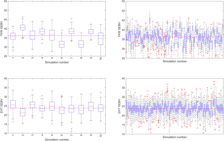
The simulations are stochastic because they model stochastic recombination events. Figure 10 (right panels) depicts the distribution of breeding values in the final generation for 100 simulations using the same starting population but different random seeds. The left panels provide a closer look at the first 10 simulations. As expected, there is variation around the average performance across all simulations. The average of the first 10 simulations is similar to the average of all 100 simulations, suggesting that the results are repeatable.
Figure 10.
Population GEBV box-plots for 10 and 100 independent simulations (left and right panels, respectively). Selection and mating decisions are optimized using MT-LAS method [with an objective of maximizing TKW and having a constraint on EHT (lower-bound 20 and upper-bound 30, similar to case 1)]. The purple dashed line demonstrates the average of GEBVs across all simulations.
Footnotes
Communicating editor: H. Daetwyler
Literature Cited
- Akdemir D., and Sánchez J. I., 2016. Efficient breeding by genomic mating. Front. Genet. 7: 210 10.3389/fgene.2016.00210 [DOI] [PMC free article] [PubMed] [Google Scholar]
- Akdemir D., Beavis W., Fritsche-Neto R., Singh A. K., and Isidro-Sánchez J., 2019. Multi-objective optimized genomic breeding strategies for sustainable food improvement. Heredity 122: 672–683. 10.1038/s41437-018-0147-1 [DOI] [PMC free article] [PubMed] [Google Scholar]
- Bates D., Mächler M., Bolker B., and Walker S., 2015. Fitting linear mixed-effects models using lme4. J. Stat. Softw. 67: 1–48. 10.18637/jss.v067.i01 [DOI] [Google Scholar]
- Brascamp E., 1984. Selection indices with constraints. Anim. Breed. Abst. 52: 645–654. [Google Scholar]
- Browning B., and Browning S., 2008. A unified approach to genotype imputation and haplotype-phase inference for large data sets of trios and unrelated individuals. American Journal of Human Genetics 84: 210–223. [DOI] [PMC free article] [PubMed] [Google Scholar]
- Burgess J. C., and West D., 1993. Selection for grain yield following selection for ear height in maize. Crop Sci. 33: 679–682. 10.2135/cropsci1993.0011183X003300040006x [DOI] [Google Scholar]
- Chang C. C., Chow C. C., Tellier L. C., Vattikuti S., Purcell S. M. et al. , 2015. Second-generation plink: rising to the challenge of larger and richer datasets. Gigascience 4: 7 10.1186/s13742-015-0047-8 [DOI] [PMC free article] [PubMed] [Google Scholar]
- Cowling W. A., Li L., Siddique K. H., Banks R. G., and Kinghorn B. P., 2019. Modeling crop breeding for global food security during climate change. Food Energy Secur. 8: e00157 10.1002/fes3.157 [DOI] [Google Scholar]
- Daetwyler H. D., Hayden M. J., Spangenberg G. C., and Hayes B. J., 2015. Selection on optimal haploid value increases genetic gain and preserves more genetic diversity relative to genomic selection. Genetics 200: 1341–1348. 10.1534/genetics.115.178038 [DOI] [PMC free article] [PubMed] [Google Scholar]
- Fernando R., and Garrick D., 2009. Gensel—user manual for a portfolio of genomic selection related analyses. Technical report. Available at: http://bigs.ansci.iastate.edu/bigsgui. Accessed: June 13, 2017.
- Goddard M., 2009. Genomic selection: prediction of accuracy and maximisation of long term response. Genetica 136: 245–257. 10.1007/s10709-008-9308-0 [DOI] [PubMed] [Google Scholar]
- Goiffon M., Kusmec A., Wang L., Hu G., and Schnable P. S., 2017. Improving response in genomic selection with a population-based selection strategy: optimal population value selection. Genetics 206: 1675–1682. 10.1534/genetics.116.197103 [DOI] [PMC free article] [PubMed] [Google Scholar]
- Hayes, B., R. Shepherd, S. Newman, and B. Kinghorn, 1998 A tactical approach to improving long term response in across breed mating plans. In: Proceedings of the Sixth World Congress on Genetics Applied to Livestock Production, Armidale, Australia, vol. 23, 439–442.
- Hayes B., Shepherd R., and Newman S., 2002. Look ahead mate selection schemes for multi-breed beef populations. Anim. Sci. 74: 13–23. 10.1017/S1357729800052206 [DOI] [Google Scholar]
- Hazel L. N., 1943. The genetic basis for constructing selection indexes. Genetics 28: 476–490. [DOI] [PMC free article] [PubMed] [Google Scholar]
- Hazel L., and Lush J. L., 1942. The efficiency of three methods of selection. J. Hered. 33: 393–399. 10.1093/oxfordjournals.jhered.a105102 [DOI] [Google Scholar]
- Itoh Y., and Yamada Y., 1988. Linear selection indices for non-linear profit functions. Theor. Appl. Genet. 75: 553–560. 10.1007/BF00289120 [DOI] [Google Scholar]
- Ivkovich M., and Koshy M., 2002. Optimization of multiple trait selection in western hemlock (tsuga heterophylla (raf.) sarg.) including pulp and paper properties. Ann. For. Sci. 59: 577–582. 10.1051/forest:2002043 [DOI] [Google Scholar]
- Jannink J.-L., Orf J., Jordan N. R., and Shaw R. G., 2000. Index selection for weed suppressive ability in soybean. Crop Sci. 40: 1087–1094. 10.2135/cropsci2000.4041087x [DOI] [Google Scholar]
- Kempthorne O., and Nordskog A. W., 1959. Restricted selection indices. Biometrics 15: 10–19. 10.2307/2527598 [DOI] [Google Scholar]
- Kinghorn B., and Shepherd R. K., 1999. Mate selection for the tactical implementation of breeding programs. Proceedings of the Advancement of Animal Breeding and Genetics 13: 130–133. [Google Scholar]
- Kinghorn B. and Kinghorn A., 2016. Instructions for matesel. Available at https://www.matesel.com/content/documentation/MateSelInstructions.pdf.
- Kusmec A., Srinivasan S., Nettleton D., and Schnable P. S., 2017. Distinct genetic architectures for phenotype means and plasticities in zea mays. Nat. Plants 3: 715–723. 10.1038/s41477-017-0007-7 [DOI] [PMC free article] [PubMed] [Google Scholar]
- Lee M., Sharopova N., Beavis W. D., Grant D., Katt M. et al. , 2002. Expanding the genetic map of maize with the intermated b73× mo17 (ibm) population. Plant Mol. Biol. 48: 453–461. 10.1023/A:1014893521186 [DOI] [PubMed] [Google Scholar]
- Long J., Holland J. B., Munkvold G. P., and Jannink J.-L., 2006. Responses to selection for partial resistance to crown rust in oat. Crop Sci. 46: 1260 10.2135/cropsci2005.06-0169 [DOI] [Google Scholar]
- Makowsky R., Pajewski N. M., Klimentidis Y. C., Vazquez A. I., Duarte C. W. et al. , 2011. Beyond missing heritability: prediction of complex traits. PLoS Genet. 7: e1002051 10.1371/journal.pgen.1002051 [DOI] [PMC free article] [PubMed] [Google Scholar]
- Meuwissen T. H. E., Hayes B. J., and Goddard M. E., 2001. Prediction of total genetic value using genome-wide dense marker maps. Genetics 157: 1819–1829. [DOI] [PMC free article] [PubMed] [Google Scholar]
- Meuwissen T., Hayes B., and Goddard M., 2016. Genomic selection: a paradigm shift in animal breeding. Anim. Front. 6: 6–14. 10.2527/af.2016-0002 [DOI] [Google Scholar]
- Moav R., and Hill W., 1966. Specialised sire and dam lines. iv. selection within lines. Anim. Sci. 8: 375–390. 10.1017/S000335610003806X [DOI] [Google Scholar]
- Moeinizade S., Hu G., Wang L., and Schnable P. S., 2019. Optimizing selection and mating in genomic selection with a look-ahead approach: an operations research framework. G3 (Bethesda) 9: 2123–2133. 10.1534/g3.118.200842 [DOI] [PMC free article] [PubMed] [Google Scholar]
- Moeinizade S., Wellner M., Hu G., and Wang L., 2020. Complementarity-based selection strategy for genomic selection. Crop Sci. 60: 149–156. 10.1002/csc2.20070 [DOI] [Google Scholar]
- Pasternak H., and Weller J., 1993. Optimum linear indices for non-linear profit functions. Anim. Sci. 56: 43–50. 10.1017/S0003356100006140 [DOI] [Google Scholar]
- Schaeffer L., 2006. Strategy for applying genome-wide selection in dairy cattle. J. Anim. Breed. Genet. 123: 218–223. 10.1111/j.1439-0388.2006.00595.x [DOI] [PubMed] [Google Scholar]
- Sharma R., and Duveiller E., 2003. Selection index for improving helminthosporium leaf blight resistance, maturity, and kernel weight in spring wheat. Crop Sci. 43: 2031–2036. 10.2135/cropsci2003.2031 [DOI] [Google Scholar]
- Shepherd R., and Kinghorn B., 1998. A tactical approach to the design of crossbreeding programs. In Proceedings of the sixth world congress on genetics applied to livestock production, volume 25, pp. 431–438. [Google Scholar]
- Suontama, M., B. Kinghorn, W. Cowling, and H. Dungey, 2018 Tactical desired gains for control of red needle cast in radiata pine under optimal contributions selection. In: Proceedings of the World Congress on Genetics Applied to Livestock Production, vol. Electronic Poster Session - Biology - Disease Resistance 3, p. 375, 2018.
- Villanueva B., and Woolliams J., 1997. Optimization of breeding programmes under index selection and constrained inbreeding. Genet. Res. 69: 145–158. 10.1017/S0016672397002656 [DOI] [Google Scholar]
- Wang L., Zhu G., Johnson W., and Kher M., 2018. Three new approaches to genomic selection. Plant Breed. 137: 673–681. 10.1111/pbr.12640 [DOI] [Google Scholar]
- Weller, J., H. Pastermak, and A. Groen, 1996 Selection indices for non-linear breeding objectives, selection for optima. Proceedings of the International Workshop on Genetic Improvement of Functional Traits in Cattle, Gembloux, Belgium. Interbull Bull 12: 206–214. [Google Scholar]
- Wilton J., Evans D. A., and Van Vleck L., 1968. Selection indices for quadratic models of total merit. Biometrics 24: 937–949. 10.2307/2528881 [DOI] [Google Scholar]
- Yan W., and Frégeau-Reid J., 2008. Breeding line selection based on multiple traits. Crop Sci. 48: 417–423. 10.2135/cropsci2007.05.0254 [DOI] [Google Scholar]
- Yang J., Ramamurthy R. K., Qi X., Fernando R. L., Dekkers J. C. et al. , 2018. Empirical comparisons of different statistical models to identify and validate kernel row number-associated variants from structured multi-parent mapping populations of maize. G3: Genes, Genomes. Genetics 8: 3567–3575. [DOI] [PMC free article] [PubMed] [Google Scholar]
- Yu J., Holland J. B., McMullen M. D., and Buckler E. S., 2008. Genetic design and statistical power of nested association mapping in maize. Genetics 178: 539–551. 10.1534/genetics.107.074245 [DOI] [PMC free article] [PubMed] [Google Scholar]
Associated Data
This section collects any data citations, data availability statements, or supplementary materials included in this article.
Data Availability Statement
The authors state that all data necessary for confirming the conclusions presented in the article are represented fully within the article. Data are available at figshare (DOI: 10.25380/iastate.12145752).


