A fractional-order SEIHDR model for COVID-19 with inter-city networked coupling effects

Abstract

In the end of 2019, a new type of coronavirus first appeared in Wuhan. Through the real-data of COVID-19 from January 23 to March 18, 2020, this paper proposes a fractional SEIHDR model based on the coupling effect of inter-city networks. At the same time, the proposed model considers the mortality rates (exposure, infection and hospitalization) and the infectivity of individuals during the incubation period. By applying the least squares method and prediction-correction method, the proposed system is fitted and predicted based on the real-data from January 23 to March $18-m$ where m represents predict days. Compared with the integer system, the non-network fractional model has been verified and can better fit the data of Beijing, Shanghai, Wuhan and Huanggang. Compared with the no-network case, results show that the proposed system with inter-city network may not be able to better describe the spread of disease in China due to the lock and isolation measures, but this may have a significant impact on countries that has no closure measures. Meanwhile, the proposed model is more suitable for the data of Japan, the USA from January 22 and February 1 to April 16 and Italy from February 24 to March 31. Then, the proposed fractional model can also predict the peak of diagnosis. Furthermore, the existence, uniqueness and boundedness of a nonnegative solution are considered in the proposed system. Afterward, the disease-free equilibrium point is locally asymptotically stable when the basic reproduction number $R_0\le 1$, which provide a theoretical basis for the future control of COVID-19.

Introduction

A infectious disease caused by a new coronavirus was discovered firstly in Wuhan, China, in the end of 2019. Contrary to the initial report [1], it is indeed spread from person to person through frequent interpersonal communication [2]. Then, it quickly spread all over the word. By 5 February, 2020, more than 24,550 had been confirmed. Since January 23, 2020, the Wuhan government has gradually implemented city-wide quarantine, which has greatly suppressed the spread of the virus.

As the main transportation hub in central China, Wuhan has a large population movement during the Spring Festival. During the transmission of the new coronavirus, population migration caused by geographical factors has added fundamental difficulties for the prevention and intervention of this epidemic, such as the domestic passenger flow from Wuhan is estimated at 5 million during the Spring Festival, which makes it difficult for following the infected people. Prasse et al. studied a discrete epidemic model with network to describe this infectious disease and their work pointed out that the epidemic model with network helped to accurately predict the outbreak of epidemics [3]. Peng et al. found that the first appearance of COVID-19 could be dated back to the beginning of December 2019 in China by a generalized SEIR model [4]. Furthermore, the basic reproduction number $R_0$ represents number of cases in which an infected individual is expected to have a second infection in a fully susceptible population. If $R_0\le 1$, an infected person, on average, infects fewer than one infection in its infectious period, and the epidemic will not exist. Conversely, if $R_0>1$, each infected individual infects more than one infected individual, and the disease will affect the entire population [5]. At present, there are a large number of articles that estimate the basic reproduction number $R_0$ to further determine whether COVID-19 will widespread in the population [6–8]. Meanwhile, during the transmission of infectious diseases, susceptible people come into contact with infected people and are infected with a probability. A great deal of evidence shows that incidence rates are an important method for describing infectious diseases [9–11]. Bilinear incidence rate is often used in the modeling process of COVID-19 because of its high infectivity. The incubation period of the infected person in the traditional SEIR model is not infectious, but there is already evidence that for COVID-19, the incubation period is very high infectious [12]. Not only that, due to various conditions, all patients infected with COVID-19 could not be sent to the hospital, and infected individuals have a high mortality rate before hospitalization.

It is worth noting that in the classic integer-order epidemic model, the state of the model does not depend on the history. However, not only does the infectious diseases depends on its current state, but also on its past state in real life. At the same time, the fractional order system can describe the change of the system whose instantaneous rate of change depended on the past state. This way of description is called the memory effect [13]. And it is confirmed that the fractional model perfectly fits the test data of memory phenomena in different disciplines by using numerical least square method. That is, a physical meaning of the fractional-order is an index of memory [14]. A large number of articles have discussed the stability of fractional order systems in different ways [15–17], such as Jan et al. concerned with some stability properties of linear autonomous fractional differential and difference systems involving derivative operators of the Riemann–Liouville type and they showed discretizations based on backward differences can retain the key qualitative properties of underlying fractional differential systems [15], and Deng et al. derived the sufficient conditions for the local asymptotical stability of nonlinear fractional differential equations, including Riemann–Liouville fractional order and Caputo fractional order derivative [16]. Furthermore, Smethurst et al. found that the waiting time for patients follows the power law model [18]. And the power law distribution $P[J_n>t]=B{x}^{-\alpha }$ generates Caputo fractional-order derivative ${}_{t_0}^C{D}_t^{\alpha }$ of the same order [19]. When dealing with practical problems, Caputo fractional order and integer order derivatives have the same initial conditions, which has a specific physical meaning. At the same time, the Caputo derivative of its constant is zero. More importantly, the accuracy of Caputo derivative can supersede the integer derivative caused by its change and non-local behavior. Angstmann et al. derived a fractional-order infectivity SIR model from a stochastic process and they found the fractional derivative appears in the generalized master equations of a continuous time random walk through SIR compartments, with a power-law function in the infectivity [20]. Khan et al. described the interaction between bats and unknown hosts, people to people, and the source of infection (seafood market), and their work shown fractional model played an important role in limiting the number of infected people [21]. Chen et al. established a fractional delay dynamic system (FTDD) to describe COVID-19, and they used reconstruction coefficients to predict the spread of new coronaviruses COVID-19 [22]. Amjad et al. constructed the fractional order COVID-19 model. In their work, the effects of preventive measures, various mitigation measures are estimated, and future outbreaks and potential control strategies are predicted [23]. A fractional SEIQRD model is analyzed by Xu et al., which is of guiding significance for predicting the possible outbreaks of some epidemic diseases [24].

To incorporate the time fractional order and the coupling effect between cities, a SEIHDR epidemic model is established to study the dynamic behavior of COVID-19. Many studies on COVID-19 shown that not only infected individuals are infectious, but people in the incubation period have same infectivity with infected individuals. Therefore, the infectivity of the incubation period is considered here. Further, the mortality of different individuals (exposed, infected and hospitalization) is considered in this model. Furthermore, during the outbreak of COVID-19, due to the limitation of various resources, the patients with infection cannot be diagnosed immediately and the patients with diagnosis cannot be hospitalized immediately, all need waiting time. Thus, from the analysis made above, a fractional inter-city network SEIHDR model for COVID-19 is established. Then, the fractional inter-city network model is verified to be rational by several numerical examples with the official data [25]. Compared with the integer system, the non-network fractional model has been verified to fit the data of Beijing, Shanghai, Wuhan and Huanggang better. The analysis with inter-city network shows that the proposed system may not have a positive effect on the spread of viruses in China, but may be important to other countries. Finally, the stability of the proposed system is analyzed through $R_0$, which has theoretical significance for further intervention and prevention of this infectious disease.

The rest of the article is organized as follows. COVID-19’s SEIHDR fractional model is established in Sect. 2. Then, some dynamic behaviors of the proposed system are analyzed in Sect. 3. In Sect. 4, numerical simulations are provided to illustrate the theoretical results. Finally, the conclusion is held in Sect. 5.

Model development

It has been found that the fractional-order derivatives have a wide range of applications in the modeling of many asynchronous dynamic processes, such as engineering, biology, medicine and many other fields [26–30]. Before presenting the fractional epidemic model, some necessary preliminaries are introduced.

Preliminaries

This section begins with some definitions and results.

Definition 2.1

[31] The Gamma function satisfies the following equation:

$$\begin{array}{c}\hfill \Gamma (\alpha )={\int }_0^{\infty }{x}^{\alpha -1}{e}^{-x}\mathrm{d}x.\end{array}$$

Definition 2.2

[31] For $\forall t>t_0$, the Caputo fractional-order derivative of order $\alpha$ ($n-1<\alpha <n)$ for a function $g(t)\in \mathbb{R}$ is defined by

$$\begin{array}{c}\hfill {}_{t_0}^C{D}_t^{\alpha }g\left(t\right)=\frac{{\mathrm{d}}^{\alpha }g\left(t\right)}{\mathrm{d}{t}^{\alpha }}=\frac{1}{\Gamma \left(n-\alpha \right)}{\int }_{t_0}^t\frac{g^{(n)}}{{\left(t-s\right)}^{\alpha -n+1}}\mathrm{d}s.\end{array}$$

Remark 2.1

If $\alpha =n$,

$$\begin{array}{c}\hfill {}_{t_0}^C{D}_t^{\alpha }g\left(t\right)=g^{(n)}(t).\end{array}$$

Definition 2.3

[32] Consider the Caputo fractional dynamical system:

$$\begin{array}{c}\hfill {}_{t_0}^C{D}_t^{\alpha }x(t)=g(t,x),x(t_0)\ge 0,\end{array}$$

a constant $x^{\ast }$ is an equilibrium point of the above system if and only if $g(t,x^{\ast })=0$.

Lemma 2.1

[33] The fractional-order system is considered as followed:

$$\begin{array}{c}\hfill {}_{t_0}^C{D}_t^{\alpha }x(t)=g(t,x),t_0>0,\end{array}$$

with the initial condition $x(t_0)=x_0$, where $\alpha \in (0,1]$ and $g:[t_0,\infty )\times \Omega \to {\mathbb{R}}^n,\Omega \in {\mathbb{R}}^n$. If g(t, x) satisfies the Lipschitz condition on x, the above system has a unique solution.

Lemma 2.2

[34] Consider the following fractional-order system:

$$\begin{array}{c}\hfill {}_{t_0}^C{D}_t^{\alpha }x(t)=g(x),x(t_0)=x_0,\end{array}$$

where $0<\alpha \le 1$, $x\in \mathbb{R}$. The equilibrium points are locally asymptotically stable if and only if all eigenvalues $\lambda$ of the Jacobian matrix $J=\frac{\partial g}{\partial x}$ satisfy the following equation:

$$\begin{array}{c}\hfill |arg(\lambda )|>\frac{\alpha \pi }{2}.\end{array}$$

System description

In December 2019, a new coronavirus was first discovered in Wuhan, China. There are a large number of epidemic models that describe the spread of this infectious disease [35]. And the spread of COVID-19 started during the Chinese New Year, and the massive population movement had made the connection between cities closer. Meanwhile, Wuhan, the most severely affected area, as a major transportation hub in central China, COVID-19 is mainly spread by means of transportation. Therefore, it is necessary to establish an inter-city network to observe the transmission of this infectious disease. Due to the limitation of medicine, latent individuals and infection individuals cannot be hospitalized immediately, which will increase the mortality rate. In addition, Tang et al. considered that the incubator of COVID-19 infection is highly infectious [12]. From the analysis made above, a fractional inter-city network SEIHDR epidemic model is constructed as follows:

$$\begin{array}{c}\hfill \begin{array}{c}\hfill \left\{\begin{array}{c}{}_0^C{D}_t^{\alpha }{S}_k={\Lambda }_k-\sum _{j=1}^n{\beta }_{\mathit{kj}}^{\alpha }\left(\frac{S_k{I}_j}{N_k},+,\frac{S_k{E}_j}{N_k}\right)-{\mu }_k^{\alpha }{S}_k,\hfill \\ {}_0^C{D}_t^{\alpha }{E}_k=\sum _{j=1}^n{\beta }_{\mathit{kj}}^{\alpha }\left(\frac{S_k{I}_j}{N_k},+,\frac{S_k{E}_j}{N_k}\right)-{\mu }_{1k}^{\alpha }{E}_k-r_k^{\alpha }{E}_k,\hfill \\ {}_0^C{D}_t^{\alpha }{I}_k=r_k^{\alpha }{E}_k-{\delta }_k^{\alpha }{I}_k-{\mu }_{2k}^{\alpha }{I}_k,\hfill \\ {}_0^C{D}_t^{\alpha }{H}_k={\delta }_k^{\alpha }{I}_k-{\lambda }_k^{\alpha }(t)H_k-{\kappa }_k^{\alpha }(t)H_k,\hfill \\ {}_0^C{D}_t^{\alpha }{R}_k={\lambda }_k^{\alpha }(t)H_k,\hfill \\ {}_0^C{D}_t^{\alpha }{D}_k={\mu }_k^{\alpha }{S}_k+{\mu }_{1k}^{\alpha }{E}_k+{\mu }_{2k}^{\alpha }{I}_k+{\kappa }_k^{\alpha }(t)H_k,\hfill \end{array}\right)\end{array}\end{array}$$ 1

with the initial condition

$$\begin{array}{c}\hfill \begin{array}{cc}& S_{\mathrm{k}}(0)=S_{\mathrm{k}}(0)\ge 0,E_{\mathrm{k}}(0)=E_{\mathrm{k}}(0)\ge 0,\hfill \\ \hfill & I_{\mathrm{k}}(0)=I_{\mathrm{k}}(0)\ge 0,H_{\mathrm{k}}(0)=H_{\mathrm{k}}(0)\ge 0,\hfill \\ \hfill & R_{\mathrm{k}}(0)=R_{\mathrm{k}}(0)\ge 0,D_{\mathrm{k}}(0)=D_{\mathrm{k}}(0)\ge 0.\hfill \end{array}\end{array}$$ 2

The city k’s total population is presented by $N_k$ that is classified into $S_k(t)$, $E_k(t)$, $I_k(t)$, $H_k(t)$, $D_k(t)$ and $R_k(t)$ denoted the class of susceptible individuals, exposed individuals, infective individuals (infected but not hospitalized), hospitalization individuals, death individuals and recovered individuals, respectively. The susceptible individual $S_k$ contact with $E_j$ and $I_j$ then infected by ${\sum }_{j=1}^n{\beta }_{\mathit{kj}}^{\alpha }(\frac{S_k{I}_j}{N_k}+\frac{S_k{E}_j}{N_k})$, where ${\beta }_{\mathit{kj}}^{\alpha }$ is the transmission coefficient. The dead individual $D_k$ includes death during susceptible ${\mu }_k^{\alpha }{S}_k$, exposure ${\mu }_{1k}^{\alpha }{E}_k$, infection ${\mu }_{2k}^{\alpha }{I}_k$, and hospitalization ${\kappa }_k^{\alpha }(t)H_k$, where ${\mu }_k$ denotes the natural death rates, ${\mu }_{\mathit{ik}}^{\alpha }$ $(i=1,2)$ and ${\kappa }_k^{\alpha }(t)$ imply the disease-related mortality. The parameter ${\Lambda }_k$ denotes the inflow number of susceptible individuals; ${\lambda }_k^{\alpha }$ be the recovery rate; $r_k^{\alpha }$ imply the transit rate of the exposed class $E_k$; ${\delta }_k$ denote hospitalization rate. Furthermore, ${\beta }_{\mathit{kj}}^{\alpha }$, ${\mu }_{\mathit{ik}}^{\alpha }$, ${\delta }_k^{\alpha }$ and $r_k^{\alpha }$ are positive constants; bounded function ${\lambda }_k^{\alpha }(t)$ and ${\kappa }_k^{\alpha }(t)$ satisfy $|{\lambda }_k^{\alpha }(t)|\le M_{1k}$ and $|{\kappa }_k^{\alpha }(t)|\le M_{2k}$ for $\forall t\ge 0$, where $M_{1k}$ and $M_{2k}$ are positive constants. Without loss of generality, ${\beta }_{\mathit{kj}}^{\alpha }$, ${\mu }_k^{\alpha }$, ${\mu }_{\mathit{ik}}^{\alpha }$, $r_k^{\alpha }$, ${\delta }_k^{\alpha }$, ${\kappa }_k^{\alpha }$ and ${\lambda }_k^{\alpha }$ are still denoted as ${\beta }_{\mathit{kj}}$, ${\mu }_k$, ${\mu }_{\mathit{ik}}$, $r_k$, ${\delta }_k$, ${\kappa }_k$ and ${\lambda }_k$, respectively.

However, during the outbreak of COVID-19, individual migration has been tightly controlled, especially for the city of Wuhan to implement the closure measures, and the natural death rate of individuals is negligible compared to the death caused by COVID-19. By the above assumptions, the improved SEIHDR model is given as followed:

$$\begin{array}{c}\hfill \begin{array}{c}\hfill \left\{\begin{array}{c}{}_0^C{D}_t^{\alpha }{S}_k=-\sum _{j=1}^n{\beta }_{\mathit{kj}}\left(\frac{S_k{I}_j}{N_k},+,\frac{S_k{E}_j}{N_k}\right),\hfill \\ {}_0^C{D}_t^{\alpha }{E}_k=\sum _{j=1}^n{\beta }_{\mathit{kj}}\left(\frac{S_k{I}_j}{N_k},+,\frac{S_k{E}_j}{N_k}\right)-{\mu }_{1k}{E}_k-r_k{E}_k,\hfill \\ {}_0^C{D}_t^{\alpha }{I}_k=r_k{E}_k-{\delta }_k{I}_k-{\mu }_{2k}{I}_k,\hfill \\ {}_0^C{D}_t^{\alpha }{H}_k={\delta }_k{I}_k-{\lambda }_k(t)H_k-{\kappa }_k(t)H_k,\hfill \\ {}_0^C{D}_t^{\alpha }{R}_k={\lambda }_k(t)H_k,\hfill \\ {}_0^C{D}_t^{\alpha }{D}_k={\mu }_{1k}{E}_k+{\mu }_{2k}{I}_k+{\kappa }_k(t)H_k.\hfill \end{array}\right)\end{array}\end{array}$$ 3

Then, the transmission diagram of a fractional SEIHDR model without inter-city network for COVID-19 is shown in Fig. 1.

Fig. 1.

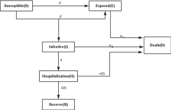
Transmission diagram for system (2)

Basic properties about the model

The dynamical analysis of the proposed system (1) is studied in this section. Here, it can be seen that the susceptible individual $S_k$, the exposed individual $E_k$, the infected individual $I_k$ and the hospitalized individual $H_k$ of system (1) are not effected by the recovered individual $R_k$ and the death class $D_k$, so the following system is considered:

$$\begin{array}{c}\hfill \begin{array}{c}\hfill \left\{\begin{array}{c}{}_0^C{D}_t^{\alpha }{S}_k={\Lambda }_k-\sum _{j=1}^n{\beta }_{\mathit{kj}}\left(\frac{S_k{I}_j}{N_k},+,\frac{S_k{E}_j}{N_k}\right)-{\mu }_k{S}_k,\hfill \\ {}_0^C{D}_t^{\alpha }{E}_k=\sum _{j=1}^n{\beta }_{\mathit{kj}}\left(\frac{S_k{I}_j}{N_k},+,\frac{S_k{E}_j}{N_k}\right)-{\mu }_{1k}{E}_k-r_k{E}_k,\hfill \\ {}_0^C{D}_t^{\alpha }{I}_k=r_k{E}_k-{\delta }_k{I}_k-{\mu }_{2k}{I}_k,\hfill \\ {}_0^C{D}_t^{\alpha }{H}_k={\delta }_k{I}_k-{\lambda }_k(t)H_k-{\kappa }_k(t)H_k,\hfill \end{array}\right)\end{array}\end{array}$$ 4

with the initial condition

$$\begin{array}{c}\hfill \begin{array}{cc}& S_{\mathrm{k}}(0)=S_{\mathrm{k}}(0)\ge 0,E_{\mathrm{k}}(0)=E_{\mathrm{k}}(0)\ge 0,\hfill \\ \hfill & I_{\mathrm{k}}(0)=I_{\mathrm{k}}(0)\ge 0,H_{\mathrm{k}}(0)=H_{\mathrm{k}}(0)\ge 0.\hfill \end{array}\end{array}$$ 5

Nonnegativity and boundedness

Before the numerical process, the existence, uniqueness and boundedness of the nonnegative solution of system (4) must be proved. Therefore, this subsection discusses the above properties of system (4).

Theorem 3.1

Consider the following initial condition:

$$\begin{array}{c}\hfill (S_k(0),E_k(0),I_k(0),H_k(0))\ge (\not\equiv )(0,0,0,0),\end{array}$$

system (4) has a unique bounded and nonnegative solution $(S_1(t),E_1(t)$, $I_1(t),H_1(t),\dots ,S_n(t),E_n(t)$, $I_n(t),H_n(t))$.

Proof

Let $N_k=S_k+E_k+I_k+H_k$. Adding all equations of system (4) yields

$$\begin{array}{c}\hfill {}_0^C{D}_t^{\alpha }{N}_k\le {\Lambda }_k-\mu N_k,\end{array}$$

which $\mu =min\{{\mu }_k,{\mu }_{1k},{\mu }_{2k},M_{1k}+M_{2k}\}$, then one has

$$\begin{array}{c}\hfill N_k(t)\le (N_k(0)-\frac{{\Lambda }_k}{\mu })E_{\alpha }(-\mu t^{\alpha })+\frac{{\Lambda }_k}{\mu }.\end{array}$$

So one has $S_k\le \frac{{\Lambda }_k}{\mu }$, $E_k\le \frac{{\Lambda }_k}{\mu }$, $I_k\le \frac{{\Lambda }_k}{\mu }$ and $H_k\le \frac{{\Lambda }_k}{\mu }$.

Let $X_{1k}=(S_k,E_k,I_k,H_k)$, $X_{2k}=({\overline{S}}_k,{\overline{E}}_k,{\overline{I}}_k,{\overline{H}}_k)$ and $F_k=(f_{1k},$ $f_{2k},f_{3k},f_{4k})$ where

$$\begin{array}{c}\hfill \begin{array}{cc}& f_{1k}={\Lambda }_k-\sum _{j=1}^n{\beta }_{\mathit{kj}}\left(\frac{S_k{I}_j}{N_k},+,\frac{S_k{E}_j}{N_k}\right)-{\mu }_k{S}_k,\hfill \\ \hfill & f_{2k}=\sum _{j=1}^n{\beta }_{\mathit{kj}}\left(\frac{S_k{I}_j}{N_k},+,\frac{S_k{E}_j}{N_k}\right)-{\mu }_{1k}{E}_k-r_k{E}_k,\hfill \\ \hfill & f_{3k}=r_k{E}_k-{\delta }_k{I}_k-{\mu }_{2k}{I}_k,\hfill \\ \hfill & f_{4k}={\delta }_k{I}_k-{\lambda }_k(t)H_k-{\kappa }_k(t)H_k.\hfill \end{array}\end{array}$$ 6

Obviously, one has

$$\begin{array}{c}\hfill \begin{array}{cc}\hfill ||F_k(X_{1k})-F_k(X_{2k})||& \le ||f_{1k}(X_{1k})-f_{1k}(X_{2k})||\hfill \\ \hfill & +||f_{2k}(X_{1k})-f_{2k}(X_{2k})||\hfill \\ \hfill & +||f_{3k}(X_{1k})-f_{3k}(X_{2k})||\hfill \\ \hfill & +||f_{4k}(X_{1k})-f_{4k}(X_{2k})||\hfill \\ \hfill & \le L_k||X-\overline{X}||,\hfill \end{array}\end{array}$$ 7

where $L_k=max(L_{1k},L_{2k},L_{3k},L_{4k},L_{5k})$, $L_{1k}=\frac{2{\beta }_{\mathit{kj}}{M}_k}{N_k}+{\mu }_k$, $L_{2k}=L_{1k}+{\mu }_{1k}+r_k$, $L_{3k}=r_k+{\mu }_{2k}+{\delta }_k$, $L_{4k}=M_{1k}+M_{2k}$. So $F_k$ satisfies the Lipschitz condition on $X_k$. Then, system (4) has a unique bounded solution ${(S_k,E_k,I_k,H_k)}_{1\le k\le n}$.

Further, the auxiliary system is considered as followed:

$$\begin{array}{c}\hfill \begin{array}{c}\hfill \left\{\begin{array}{c}{}_0^C{D}_t^{\alpha }{\underset{\_}{S}}_k=-\sum _{j=1}^n{\beta }_{\mathit{kj}}(\frac{{\underset{\_}{S}}_k{\underset{\_}{I}}_j}{N_k}+\frac{{\underset{\_}{S}}_k{\underset{\_}{E}}_j}{N_k})-{\mu }_k{\underset{\_}{S}}_k,\hfill \\ {}_0^C{D}_t^{\alpha }{\underset{\_}{E}}_k=\sum _{j=1}^n{\beta }_{\mathit{kj}}(\frac{{\underset{\_}{S}}_k{\underset{\_}{I}}_j}{N_k}+\frac{{\underset{\_}{S}}_k{\underset{\_}{E}}_j}{N_k})-{\mu }_{1k}{\underset{\_}{E}}_k-r_k{\underset{\_}{E}}_k,\hfill \\ {}_0^C{D}_t^{\alpha }{\underset{\_}{I}}_k=r_k{\underset{\_}{E}}_k-{\delta }_k{\underset{\_}{I}}_k-{\mu }_{2k}{\underset{\_}{I}}_k,\hfill \\ {}_0^C{D}_t^{\alpha }{\underset{\_}{H}}_k={\delta }_k{\underset{\_}{I}}_k-{\lambda }_k{\underset{\_}{H}}_k-{\kappa }_k{\underset{\_}{H}}_k,\hfill \\ {\underset{\_}{S}}_k={\underset{\_}{E}}_k={\underset{\_}{I}}_k={\underset{\_}{H}}_k=0.\hfill \end{array}\right)\end{array}\end{array}$$

Through the comparison theorem, it is found that

$$\begin{array}{c}\hfill (S_k,E_k,I_k,H_k)\ge ({\underset{\_}{S}}_k,{\underset{\_}{E}}_k,{\underset{\_}{I}}_k,{\underset{\_}{H}}_k)=(0,0,0,0).\end{array}$$

Thus, it can be concluded that $S_k\ge 0$, $E_k\ge 0$, $I_k\ge 0$ and $H_k\ge 0$ for $k=1,2,\dots ,n$. $\square$

Stability analysis

Now, exploring the stability of the system (4) through the basic reproduction number $R_0$. Obviously, the disease-free equilibrium for system (4) is $E^0=(\frac{{\Lambda }_1}{{\mu }_1},0,0,0,\dots ,\frac{{\Lambda }_n}{{\mu }_n},0,0,$ 0).

Theorem 3.2

The basic reproduction number $R_0$ of system (4) is

$$\begin{array}{c}\hfill R_0=\rho (F_1(V_{21}-V_{20}){(V_{21}{V}_{10})}^{-1}),\end{array}$$

where $F_1={(\frac{{\beta }_{\mathit{kj}}{\Lambda }_k}{N_k{\mu }_k})}_{1\le k,j\le n}$, $V_{10}=\mathrm{diag}({\mu }_{11}+r_1,\dots ,{\mu }_{1n}+r_n)$, $V_{20}=\mathrm{diag}(-r_1,\dots ,-r_n)$, $V_{21}=\mathrm{diag}({\delta }_1+{\mu }_{21},\dots ,{\delta }_n+{\mu }_{2n})$ and the spectral radius $\rho (F_1(V_{21}-V_{20}){(V_{21}{V}_{10})}^{-1})$.

Proof

Let $F_0=({\sum }_{j=1}^n\frac{{\beta }_{\mathit{kj}}{S}_k(I_j+E_j)}{N_k})$, $V_{01}=(({\mu }_{1k}+r_k)E_k)$, $V_{02}=({\delta }_k{I}_k+{\mu }_{2k}{I}_k-r_k{E}_k)$ and $V_{03}=({\lambda }_k{H}_k+{\kappa }_k{H}_k-{\delta }_k{I}_k)$ $(k=1,2,\dots ,n)$. Then, taking the derivative of $F_0$, $V_{01}$, $V_{02}$ and $V_{03}$ with respect to $E_k$, $I_k$ and $H_k$ $(k=1,2,\dots ,n)$ at $E^0$, it can be concluded that

$$\begin{array}{cc}\hfill F=& \left(\begin{array}{ccc}{F}_1& F_1& 0\\ 0& 0& 0\\ 0& 0& 0\end{array}\right),\hfill \\ \hfill V=& (V_1,V_2.V_3),\hfill \end{array}$$

where $V_1=(V_{10},0,0)$, $V_2=(V_{20},V_{21},0)$, $V_3=(0,V_{30},V_{31})$, $F_1={(\frac{{\beta }_{\mathit{kj}}{\Lambda }_k}{N_k{\mu }_k})}_{n\times n}$, $V_{10}=\mathrm{diag}({\mu }_{11}+r_1,\dots ,{\mu }_{1n}+r_n)$, $V_{20}=\mathrm{diag}(-r_1,\dots ,-r_n)$, $V_{21}=\mathrm{diag}({\delta }_1+{\mu }_{21},\dots ,{\delta }_n+{\mu }_{2n})$, $V_{30}=\mathrm{diag}(-{\delta }_1,\dots ,-{\delta }_n)$ and $V_{31}=\mathrm{diag}({\lambda }_1+{\kappa }_1,\dots ,{\lambda }_n+{\kappa }_n)$. Then, according to [5], it can be yielded that

$$\begin{array}{c}\hfill R_0=\rho (F{V}^{-1})=\rho (F_1(V_{21}-V_{20}){(V_{21}{V}_{10})}^{-1}).\end{array}$$

$\square$

It is obvious to get the following theorem:

Theorem 3.3

If the basic reproduction number $R_0\le 1$, system (4) is locally stability at the disease-free equilibrium point $E^0=(\frac{{\Lambda }_1}{{\mu }_1},0,0,0,\dots ,\frac{{\Lambda }_n}{{\mu }_n},0,0,$ 0).

Proof

Consider the following Jacobian matrix of system (4) at $E^0$

$$\begin{array}{c}\hfill J^0=\left(\begin{array}{cccc}W& -F_1& -F_1& 0\\ 0& F_1-V_1& F_1& 0\\ 0& -V_{20}& -V_{21}& 0\\ 0& 0& -V_{30}& -V_{31}\end{array}\right),\end{array}$$

where $W=\mathrm{diag}(-{\mu }_1,$ $\dots ,-{\mu }_n)$. One can calculate that the eigenvalues are $s_{1k}=-{\mu }_k$ $(k=1,2,\dots ,n)$ and $s_2=-s(V_{31})$ and

$$\begin{array}{c}\hfill \begin{array}{c}{s}_3+s_4=s(F_1-V_{10}-V_{21}),\hfill \\ s_3{s}_4=s(F_1(V_{20}-V_{21})+V_{21}{V}_{10}),\hfill \end{array}\end{array}$$

where $s(V_{31})$, $s(F_1-V_{10}-V_{21})$ and $s(F_1(V_{20}-V_{21})+V_{21}{V}_{10})$ are all eigenvalues of the matrix $V_{31}$, $F_1-V_{10}-V_{21}$ and $F_1(V_{20}-V_{21})+V_{20}{V}_{21}$, respectively. Then, if $R_0\le 1$, it can be yielded that $|arg(s)|>\frac{\pi }{2}>\frac{\alpha \pi }{2}$. Thus, system (4) is locally stability at the disease-free equilibrium point $E^0=(\frac{{\Lambda }_1}{{\mu }_1},0,0,0,$ $..,\frac{{\Lambda }_n}{{\mu }_n},0,0,0)$. $\square$

Remark 3.1

When city k and city j have no communication (ie, city k is closed), the basic reproduction number of city k can be expressed as followed:

$$\begin{array}{c}\hfill R_0^k=\frac{{\beta }_{\mathit{kk}}{\Lambda }_k({\delta }_k+{\mu }_{2k}+r_k)}{({\delta }_k+{\mu }_{2k})({\mu }_{1k}+r_k){\mu }_k{N}_k}.\end{array}$$

So, $E_k^0$ is local stability when the basic reproduction number $R_0^k\le 1$.

Remark 3.2

It is evident that $R_0^k$ are dependent on ${\lambda }_k$ and ${\kappa }_k$. The sensitivity of $R_0^k$ to the other parameters ${\beta }_{\mathit{kk}}$, ${\mu }_{1k}$, $r_k$, ${\mu }_{2k}$ and ${\delta }_k$ is calculated as follows:

$$\begin{array}{cc}& A_{{\beta }_{\mathrm{kk}}}=\frac{{\beta }_{\mathrm{kk}}}{R_0}\frac{\partial R_0}{\partial {\beta }_{\mathrm{kk}}}=1,A_{{\mu }_{1\mathrm{k}}}=\frac{{\mu }_{1\mathrm{k}}}{R_0}\frac{\partial R_0}{\partial {\mu }_{1\mathrm{k}}}=-\frac{{\mu }_{1\mathrm{k}}}{{\mu }_{1\mathrm{k}}+r_k},\hfill \\ \hfill & A_{{\mu }_{2\mathrm{k}}}=\frac{{\mu }_{2\mathrm{k}}}{R_0}\frac{\partial R_0}{\partial {\mu }_{2\mathrm{k}}}=-\frac{r_k}{({\delta }_k+{\mu }_{2\mathrm{k}})({\delta }_k+{\mu }_{2\mathrm{k}}+r_k)},\hfill \\ \hfill & A_{r_{\mathrm{k}}}=\frac{r_{\mathrm{k}}}{R_0}\frac{\partial R_0}{\partial r_{\mathrm{k}}}=\frac{r_k({\mu }_{1\mathrm{k}}-{\mu }_{2\mathrm{k}}-{\delta }_k)}{({\delta }_k+{\mu }_{2\mathrm{k}}+r_k)},\hfill \\ \hfill & A_{{\delta }_{\mathrm{k}}}=\frac{{\delta }_{\mathrm{k}}}{R_0}\frac{\partial R_0}{\partial {\mu }_{2\mathrm{k}}}=-\frac{r_k{\delta }_k}{({\delta }_k+{\mu }_{2\mathrm{k}})({\delta }_k+{\mu }_{2\mathrm{k}}+r_k)},\hfill \end{array}$$

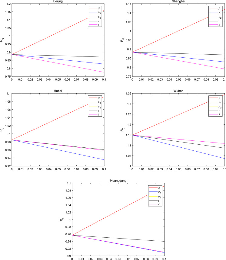
where $A_{{\beta }_{\mathit{kk}}}$, $A_{{\mu }_{1k}}$, $A_{{\mu }_{2k}}$ and $A_{{\delta }_k}$ represent the normalized sensitivity on ${\beta }_{\mathit{kk}}$, ${\mu }_{1k}$, ${\mu }_{2k}$ and ${\delta }_k$, respectively. It is worth noting that the n times’ increase on ${\beta }_{\mathit{kk}}$ leads to the n times’ increase on $R_0^k$, but the n times’ increase on ${\mu }_{1k}$, ${\mu }_{2k}$, ${\delta }_k$ and $r_k$ leads to the n times’ decrease on $R_0^k$.

Numerical analysis

It can be seen from the previous discussion that system (1) has a unique bounded solution, and the disease-free equilibrium point $E^0$ is locally asymptotically stable, which can provide theoretical support for the further control and prediction of COVID-19. Then, the numerical solutions of system (1) are analyzed by least squares method [36] and predictor-correctors scheme. In order to predictions, it is possible to move the data by a fixed date m before March 18. Determine predictions are made based on data of $18-m$ from January 23 to March 18, 2020. Then, it can be predict the number of people diagnosed on March 18 and m represents the predicted number of days. Like in [12], the disease-related mortality $\kappa (t)$ and the cure rates $\lambda (t)$ are time-varying functions as

$$\begin{array}{c}\hfill \begin{array}{c}\hfill \kappa (t)={\kappa }_0{e}^{-{\kappa }_{1}t},\lambda (t)={\lambda }_0(1-e^{{\lambda }_{1}t}),\end{array}\end{array}$$ 8

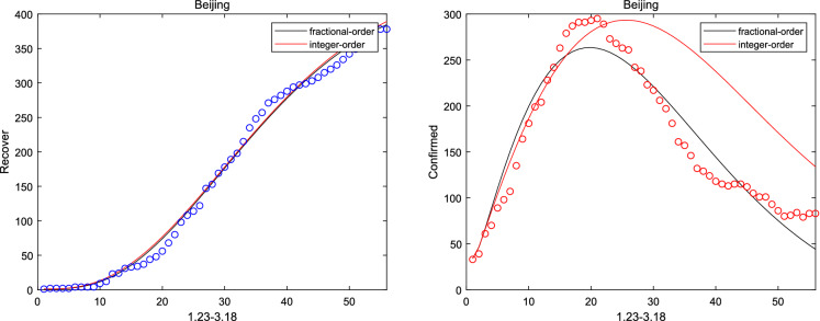
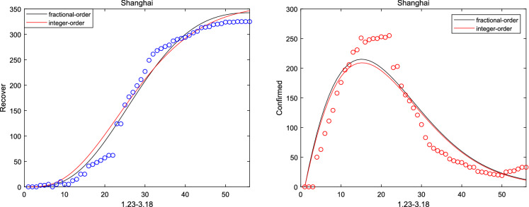
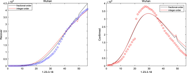
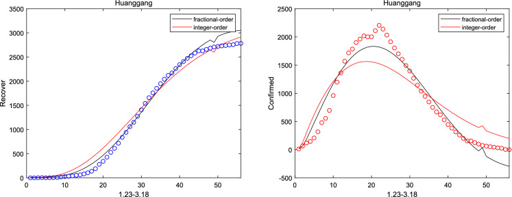
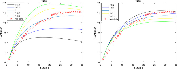
where ${\lambda }_0$ and ${\kappa }_0$ are initial cure rate and mortality. Considering without the network, it can be seen that the fitting effect of the fractional system (3) on the peak value and the peak time is a little bit better than that of the integer system (ie $\alpha =1$) from Figs. 2, 3, 4, 5 and 6. And the relative error between the real-date and the numerical solutions of $\alpha =1$ and $\alpha \ne 1$ can be seen from Table 1. Particularly, corresponding the basic reproduction number $R_k^0$ and the fractional-order are shown in Table 2. Then, consistent with Remark 3.2, Fig. 7 indicates the sensitivity of $R_0^k$. Furthermore, according to Fig. 8, it is observed that the peak time and the peak value are given as the coefficient ${\beta }_{\mathit{kk}}$ and the hospitalization rate ${\delta }_k$ change. The numerical results show that strict control of individual exposure and increased detection of nucleic acid reagents play a vital role in reducing confirmed cases and delaying the peak period. However, from Fig. 8, it can also be found that the peak time reaches earlier and the peak value becomes larger as the disease coefficient ${\beta }_{\mathit{kk}}$ increases. So, the non-closed policy adopted by many countries are also reasonable

Fig. 2.

The number of recovered and confirmed for Beijing (m = 6)

Fig. 3.

The number of recovered and confirmed for Shanghai ($m=6$)

Fig. 4.

The number of recovered and confirmed for Hubei ($m=6$)

Fig. 5.

The number of recovered and confirmed for Wuhan ($m=6$)

Fig. 6.

The number of recovered and confirmed for Huanggang ($m=6$)

Table 1.

Error with the real-data and the numerical solutions

Error ($\%$)	Different country
	Beijing	Shanghai	Hubei	Wuhan	Huanggang
$\alpha =1$	23.6	34.3	21.8	19.2	78.3
$\alpha \ne 1$	5.9	14.1	16.2	19.1	49.7

Table 2.

Performance comparison with different city

Different country	Different index
	$\alpha$	$R_0$
Beijing	1.1913	0.8855
Shanghai	0.9844	0.8833
Hubei	1.4343	0.9848
Wuhan	0.9995	1.2675
Huanggang	0.0332	0.9568
America	0.7945	1.1443
Japan	0.3279	1.6346
Italy	0.7056	$1.3368\times {10}^3$

Fig. 7.

The sensitivity of the basic reproduction number

Fig. 8.

Prediction of peak in Hubei province

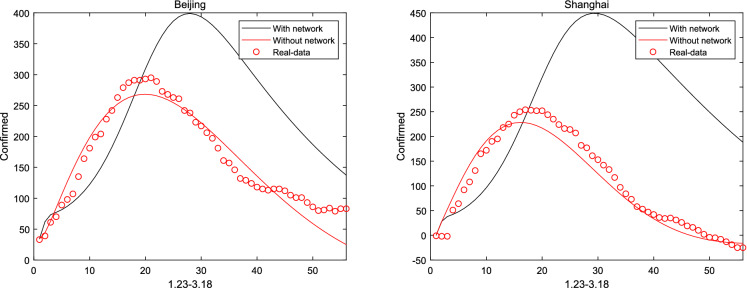
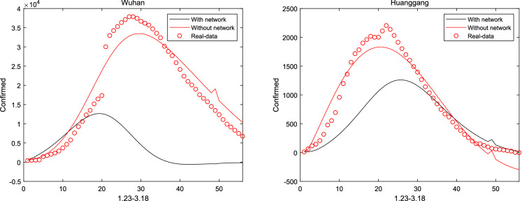
When considered Hubei and other cities interacting with each other, the communication between cities is not clear and can be identified from system (1). Then, Figs. 9 and 10 describe the network coupling between Beijing, Shanghai, Wuhan and Huanggang. It can be seen that since China closed the city on January 23, the epidemic model with network is no longer suitable for China. However, regarding the population movements in other countries, a network-based model can be established to describe the spread of the virus, which will show better performance, and this will also be the focus of future research

Fig. 9.

With and without inter-city network in Beijing and Shanghai

Fig. 10.

With and without considering inter-city network in Wuhan and Huanggang

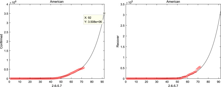
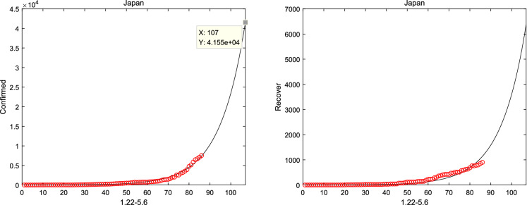
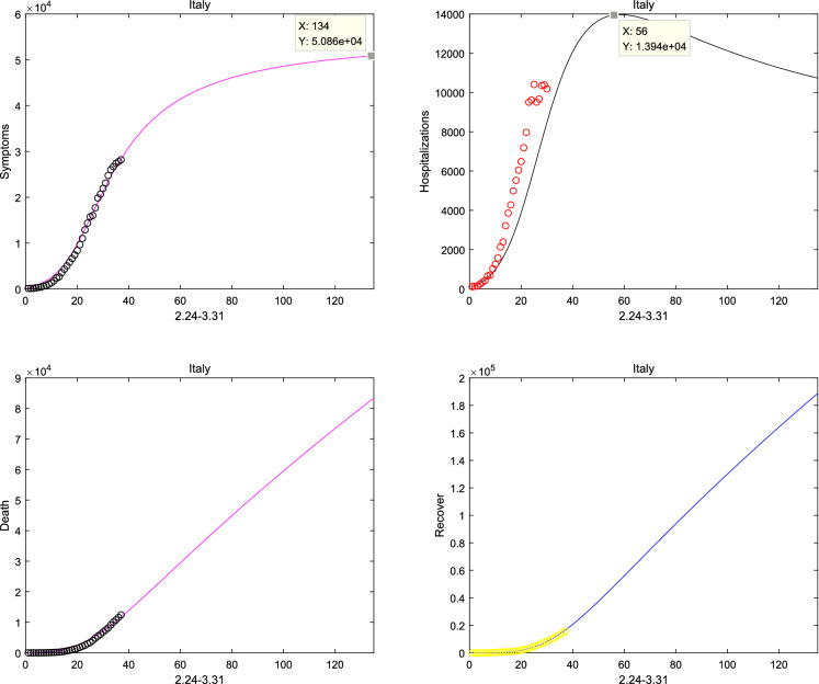
Meanwhile, considering system (1) without the natural death rate ${\mu }_k$, the short-term prediction for America and Japan is shown in Figs. 11, 12 when considered the real-date dating from 22 January and 1 February to 16 April, 2020 [37], respectively. And it can be shown from Figs. 11 and 12 that the number of confirmed and recovery individuals will keep increasing for America and Japan. Finally, the prediction is considered in Fig. 13, according to the Italian real-data of hospitalization, death and recovery from February 24 to March 31 [38]. And it is obviously that the peak time of symptomatic individuals and hospitalizations reach on 30 June and 20 April, respectively. Then, the basic reproduction number and the fractional order can be seen from Table 2, which suggests that the epidemic model of Italy, America and Japan will not disappear in a short time.

Fig. 11.

American report and forecast from 22 January to 16 April

Fig. 12.

Japan report and forecast from 1 February to 16 April

Fig. 13.

Italy report and forecast from 24 February to 31 March

Discussion

Based on the coupling effects of inter-city network in Beijing, Shanghai, Wuhan and Huanggang, this paper proposes a fractional SEIHDR model. By applying the method of least squares and prediction-correction, the numerical solution of the system (3) is compared with the actual value of Beijing, Shanghai, Hubei, Wuhan and Huanggang from January 23 to March 18, 2020. It can be found from this study that fractional systems have a better fitting effect than integer systems. Besides, based on the inter-city network, the analysis shows that the system with inter-city network could not be a better description of infectious transmission in China. At the same time, system (1) fits the data of Japan, the USA from January 22 to April 16 and Italy from February 24 to March 31, and predicts the peak value and the peak time, respectively. Moreover, the existence, uniqueness and boundedness of a nonnegative solution are established. Further, the local stability at the disease-free equilibrium point is studied by $R_0\le 1$. And the sensitivity of $R_0^k$ without network are researched to provide a theoretical basis for infectious disease control.

Although the above study may not be able to show the impact of the inter-city network-based epidemic model on disease transmission in China because of strict locking measures, it may on the whole indicates that the fractional epidemic model with network may predict more accurate than independent. Although the situation of COVID-19 can be effectively predicted in China, this study raises some questions that require further research: whether the network model can be used to predict epidemics in other regions; how medical and other factors affect the virus transmission trend. Further study how to predict and intervene in the development of epidemic situations in other countries when the dynamic model includes network effects.

Compliance with ethical standards

Conflict of interest

The authors declare no conflicts of interest.

References

- 1.Fasina FO. Novel coronavirus (2019-nCoV): what we know and what is unknown. Asian Pac. J. Trop. Med. 2020;13(3):97. doi: 10.4103/1995-7645.277795. [DOI] [Google Scholar]
- 2.Chan J, Yuan S, Kok K, To K, Chu H, Yang J, Xing F, Liu J, Yip CC, Poon R, Tsoi H, Lo S, Chan K, Poon V, Chan W, Cai JDJ, Cheng C, Chen H, Hui C, Yuen K. A familial cluster of pneumonia associated with the 2019-novel coronavirus indicating person-to-person transmission: a study of a family cluster. Lancet. 2020;395(10223):514–523. doi: 10.1016/S0140-6736(20)30154-9. [DOI] [PMC free article] [PubMed] [Google Scholar]
- 3.Prasse, B., Massimo A.A., Van Mieghem, L.M.P.: Network-based prediction of the 2019-ncov epidemic outbreak in the Chinese province Hubei. Physics and Society (2020). arxiv:2002.04482 [DOI] [PMC free article] [PubMed]
- 4.Peng, L., Yang, W., Zhang, D., Zhuge, C., Hong, L.: Epidemic analysis of COVID-19 in China by dynamical modeling. Populations and Evolution (2020). arXiv:2002.06563. 10.1101/2020.02.16.20023465
- 5.van den Driessche P, Watmough J. Reproduction numbers and sub-threshold endemic equilibria for compartmental models of disease transmission. Math. Biosci. 2002;180(1–2):29–48. doi: 10.1016/S0025-5564(02)00108-6. [DOI] [PubMed] [Google Scholar]
- 6.Lai C, Shih T, Ko W, Tang H, Hsueh P. Severe acute respiratory syndrome coronavirus 2 (SARS-CoV-2) and coronavirus disease-2019 (COVID-19): The epidemic and the challenges. Int. J. Antimicrob. Agents. 2020;55(3):105924. doi: 10.1016/j.ijantimicag.2020.105924. [DOI] [PMC free article] [PubMed] [Google Scholar]
- 7.Liu Y, Gayle A, Wilder-Smith A, Rocklov J. The reproductive number of COVID-19 is higher compared to SARS coronavirus. J. Travel Med. 2020;27(2):taaa021. doi: 10.1093/jtm/taaa021. [DOI] [PMC free article] [PubMed] [Google Scholar]
- 8.Sahafizadeh E, Sartoli S. Estimating the Reproduction Number of COVID-19 in Iran Using Epidemic Modeling. Cold Spring Harbor: Cold Spring Harbor Laboratory; 2020. [Google Scholar]
- 9.Anderson R, Anderson B, May R. Infectious Diseases of Humans: Dynamics and Control. Oxford: Oxford University Press; 1992. [Google Scholar]
- 10.Bailey N. The Mathematical Theory of Infectious Diseases and Its Applications. London: Charles Griffin & Company Ltd.; 1975. [Google Scholar]
- 11.Upadhyay R, Pal A, Kumari S, Roy P. Dynamics of an SEIR epidemic model with nonlinear incidence and treatment rates. Nonlinear Dyn. 2019;96(4):2351–2368. doi: 10.1007/s11071-019-04926-6. [DOI] [Google Scholar]
- 12.Tang Z, Li X, Li H. Prediction of New Coronavirus Infection Based on a Modified SEIR Model. Cold Spring Harbor: Cold Spring Harbor Laboratory; 2020. [Google Scholar]
- 13.Zhou P, Ma J, Tang J. Clarify the physical process for fractional dynamical systems. Nonlinear Dyn. 2020;100:1–12. doi: 10.1007/s11071-020-05520-x. [DOI] [Google Scholar]
- 14.Du M, Wang Z, Hu H. Measuring memory with the order of fractional derivative. Sci. Rep. 2013;3:1–3. doi: 10.1038/srep03431. [DOI] [PMC free article] [PubMed] [Google Scholar]
- 15.Jan C, Tomás K, Ludek N. Stability regions for linear fractional differential systems and their discretizations. Appl. Math. Comput. 2013;219:7012–7022. [Google Scholar]
- 16.Deng WH. Smoothness and stability of the solutions for nonlinear fractional differential equations. Nonlinear Anal. 2010;72:1768–1777. doi: 10.1016/j.na.2009.09.018. [DOI] [Google Scholar]
- 17.Huang CD, Cao JD, Xiao M, Alsaedi A, Hayat T. Bifurcations in a delayed fractional complex-valued neural network. Appl. Math. Comput. 2017;292:210–227. [Google Scholar]
- 18.Smethurst D, Williams H. Are hospital waiting lists selfregulating? Nature. 2001;410(6829):652–653. doi: 10.1038/35070647. [DOI] [PubMed] [Google Scholar]
- 19.Meerschaert M, Sikorskii A. Stochastic Models for Fractional Calculus. Berlin: De Gruyter; 2011. [Google Scholar]
- 20.Angstmann CN, Henry BI, McGann AV. A fractional-order infectivity SIR model. Phys. A. 2018 doi: 10.1016/j.physa.2016.02.029. [DOI] [PubMed] [Google Scholar]
- 21.Khan MA, Atangana A. Modeling the dynamics of novel coronavirus (2019-nCov) with fractional derivative. Alex. Eng. J. 2020 doi: 10.1016/j.aej.2020.02.033. [DOI] [Google Scholar]
- 22.Chen, Y., Cheng, J., Jiang, X., Xu, X.: The reconstruction and prediction algorithm of the fractional TDD for the local outbreak of COVID-19. Physics and Society (2020). arXiv:2002.10302
- 23.Amjad S.S., Iqbal N.S., Kottakkaran Sooppy, N.: A mathematical model of COVID-19 using fractional derivative: outbreak in India with dynamics of transmission and control. Preprints (2020). 10.20944/preprints202004.0140.v1 [DOI] [PMC free article] [PubMed]
- 24.Xu C, Yu Y, Chen Y, Lu Z. Forecast analysis of the epidemics trend of COVID-19 in the United States by a generalized fractional-order SEIR model. Nonlinear Dyn. 2020 doi: 10.1101/2020.04.24.20078493. [DOI] [PMC free article] [PubMed] [Google Scholar]
- 25.https://wjw.hubei.gov.cn/bmdt/ztzl/fkxxgzbdgrfyyq/xxfb/
- 26.Hossein K, Mohsen J. Stability analysis of a fractional order model for the HIV/AIDS epidemic in a patchy environment. J. Comput. Appl. Math. 2019;346:323–339. doi: 10.1016/j.cam.2018.06.055. [DOI] [Google Scholar]
- 27.Huo J, Zhao H, Zhu L. The effect of vaccines on backward bifurcation in a fractional order HIV model. Nonlinear Anal. Real World Appl. 2015;26:289–305. doi: 10.1016/j.nonrwa.2015.05.014. [DOI] [Google Scholar]
- 28.Yang Y, Xu LG. Stability of a fractional order SEIR model with general incidence. Appl. Math. Lett. 2020;105:106303. doi: 10.1016/j.aml.2020.106303. [DOI] [Google Scholar]
- 29.Ricardo A. Analysis of a fractional SEIR model with treatment. Appl. Math. Lett. 2018;84:56–62. doi: 10.1016/j.aml.2018.04.015. [DOI] [Google Scholar]
- 30.Sierociuk D, Skovranek T, Macias M, Podlubny I, Petras I, Dzielinski A, Ziubinski P. Diffusion process modeling by using fractional-order models. Appl. Math. Comput. 2015;257:2–11. [Google Scholar]
- 31.Podlubny I. Fractional Differential Equations. Cambridge: Academic Press; 1999. [Google Scholar]
- 32.Li Y, Chen Y, Podlubny I. Mittag–Leffler stability of fractional order nonlinear dynamic systems. Automatica. 2009;45(8):1965–1969. doi: 10.1016/j.automatica.2009.04.003. [DOI] [Google Scholar]
- 33.Li Y, Chen Y, Podlubny I. Stability of fractional-order nonlinear dynamic systems: Lyapunov direct method and generalized Mittag-Leffler stability. Comput. Math. Appl. 2010;59(5):1810–1821. doi: 10.1016/j.camwa.2009.08.019. [DOI] [Google Scholar]
- 34.Petras I. Fractional-Order Nonliear Systems: Modeling Analysis and Simulation. Beijing: Higher Education Press; 2011. [Google Scholar]
- 35.Wang, M., Qi, J.T.: A deterministic epidemic model for the emergence of COVID-19 in China (2020). 10.37473/dac/10.1101/2020.03.08.20032854
- 36.Cheynet, E.: Generalized SEIR Epidemic Model (Fitting and Computation) (2020). http://www.github.com/ECheynet/SEIR
- 37.https://github.com/CSSEGISandData/COVID-19/tree/master/csse_covid_19_data
- 38.https://github.com/pcm-dpc/COVID-19