Abstract
COVID-2019 is a global threat, for this reason around the world, researches have been focused on topics such as to detect it, prevent it, cure it, and predict it. Different analyses propose models to predict the evolution of this epidemic. These analyses propose models for specific geographical areas, specific countries, or create a global model. The models give us the possibility to predict the virus behavior, it could be used to make future response plans. This work presents an analysis of COVID-19 spread that shows a different angle for the whole world, through 6 geographic regions (continents). We propose to create a relationship between the countries, which are in the same geographical area to predict the advance of the virus. The countries in the same geographic region have variables with similar values (quantifiable and non-quantifiable), which affect the spread of the virus. We propose an algorithm to performed and evaluated the ARIMA model for 145 countries, which are distributed into 6 regions. Then, we construct a model for these regions using the ARIMA parameters, the population per 1M people, the number of cases, and polynomial functions. The proposal is able to predict the COVID-19 cases with a RMSE average of 144.81. The main outcome of this paper is showing a relation between COVID-19 behavior and population in a region, these results show us the opportunity to create more models to predict the COVID-19 behavior using variables as humidity, climate, culture, among others.
Keywords: Covid-19 epidemic, Forecast, ARIMA model, Geographic region
1. Introduction
In December 2019 in Wuhan, China started the pandemic of COVID-19, commonly known as Coronavirus, which has caused havoc around the world. World Health organization reported on June 7 [1], the virus is in 216 Countries, there are 6 750 521 active cases, and it has produced 395 779 deaths. For this reason, scientists around the world have been focused on topics such detect it [2], prevent it [3], cure it [4], and predict it [5], [6], [7], [8], [9], [10], [11], [12], [13]. To predict the coronavirus different schemes has been applied, for example in [11] proposes an approach, which is based Composite Monte Carlo enhanced by deep learning and fuzzy rule induction to predict the COVID-19, [14] detailed models for forecasting the course of the pandemic, these models demonstrate the utility of parsimonious models for early-time data. Using the official data forecasting, [15] studied the spread of COVID-19, they realized forward prediction and backward inference of the epidemic. [16] applied mathematical models and time-series to describe the outbreak among passengers and crew members on Princess Cruises Ship.
A model using early forecasting from Small Dataset is proposed by [6]. In [5] the authors proposed used ARIMA models to predict the spread around the world, in specific they use two models ARIMA (1,2,0) and ARIMA (1,0,4). An ARIMA (1,1,2) model is selected to fit the predictions in Italy by [8], [10] proposed ARIMA models to predict cases and deaths per 3 countries Italy, Turkey, and Spain. A ARIMA (2,2,2) model is used by [9] to predict the spread in India. Models for different regions of Italy are proposed by [7]. [13] uses (ARIMA) model to analyze two data sets and predict the daily new confirmed cases for the 7-day period. In [12], the authors have studied 15 countries (USA, Spain, Italy, France, Germany, United Kingdom (UK), Turkey, Iran, China, Russia, Brazil, Canada, Belgium, Netherlands and Switzerland) to predict the spread of the Coronavirus in these countries.
As we can see, advanced prediction models used ARIMA [17] to predict the spread of Coronavirus, this is because the ARIMA models give results in terms of its predictive performance. The models give us the possibility to predict the virus behavior, it could be used to make future response plans. There are countries, which have faced the COVID-19 in the same way, (Brazil and Sweden) but with totally different consequences. The differences between these countries are geographical, demographic, economic, public health, cultural, poverty, among others. These differences have caused that Brazil has 694,116 cases while Sweden has 45,133 cases on June 8. As we can see, Brazil has 15.3 times more cases than Sweden. For this fact, in this work, we propose to create a relationship between the countries and two variables more to predict the COVID-19 behavior. These variables are the geographic region and the total population in the country. The geographic regions are North America, South America, Africa, Asia and Europe. The countries in the same geographic region (continent) different variables with similar values such as quantifiable data (climate, humidity, natural regions, etc.) and other non-quantifiable (cultural similarities, similar gastronomy, among others).
We propose an algorithm to performed and evaluated the Auto-Regressive Integrated Moving Average (ARIMA) model for 145 countries, which are distributed in 6 geographic regions. The ARIMA models using the available information until April 25 2020. Next, the information is divided into 2 sets, the first set is used to create the ARIMA models and the second set is used to calculate the RMSE between the real data and predict data. The First set uses 90% of the data and the second set uses 10% of the data. Then, the calculated parameters of ARIMA models, the population per 1M people per country, the number of cases per country are used to create polynomial functions, which are able to predict the ARIMA parameters. These polynomial functions generate models for the next geographic regions: North America, South America, Africa, Oceania, Asia, and Europe.
The results are evaluated using RMSE. The main contributions can be summarized as follows:
-
•
We propose an algorithm to calculate the best ARIMA parameters per country with low RMSE.
-
•
The algorithm to calculate the best parameter of ARIMA is tested with 10% of the original data.
-
•
Our approach is analyzing 145 countries, almost 10 times more than another proposed scheme.
-
•
The approach starts analyzing particular cases (countries) to create a general case (geographic region).
-
•
Our approach is able to show a relation between the prediction error and other variables. In this work, a relation between the prediction error and the population per 1M people is shown.
The organization of the paper is as follows. Section 2 briefs the databases used. Section 3 presents the proposed approach. The paper ends with the Results, a Discussion section and Conclusion.
2. Databases
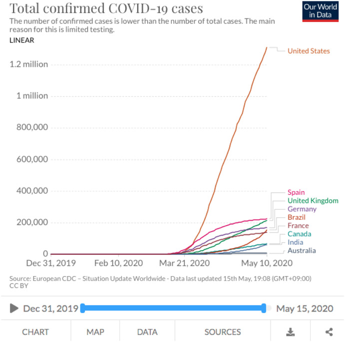
The time series created in this work using the data of “Our World in Data” [18], which is completely open access. They collect the data from the European Centre for Disease Prevention and Control (ECDC), the WHO, Johns Hopkins, United Nations, World Bank, Global Burden of Disease, Blavatnik School of Government, etc. They standardized names of countries using “Our World in Data” [18] standard entity names, they discarded detected inconsistencies in the original data, detailed documentation for each country is available [18]. Multiple time series for a country are collected, the complete COVID-19 dataset only includes the most complete number of people tested, confirmed cases and deaths. The data on the coronavirus pandemic is updated daily. “Our World in Data” has 77 charts on COVID-19. Fig. 1 shows an example of one chart. The data of charts contain information from 207 countries. Then, we can explore the statistics on COVID-19 for the countries in the world. This work uses the available information until May 28. The consulted chart is “Total and daily confirmed COVID-19 cases”, which is used to create the time series per country called “Total confirmed COVID-19 cases”. The time series start on the day when each country presented the first case of COVID-19 and finish on May 28. This fact means the length of time series are different per each country. For example, the time series of Canada starts on January 26 (123 days until May 28), Egypt time series starts on February 15 (103 days until May 28), time series of China starts on December 31 (149 days until May 28), Italy time series starts on January 31 (118 days until May 28), time series of Australia starts on January 25 (124 days until May 28), Brazil time series starts on February 26 (92 days until May 28), etc.
Fig. 1.
Example of the available information on “Our World in Data”.
This paper proposes a model per geographic region. The countries are separated in 6 regions which are North America (13 countries), South America (12 countries), Africa (43 countries), Asia (40 countries) and Europe (33 countries). To create the models per region, we use the “total population in the age groups” available in the website of United Nations [19]. The population in the age groups is added to generate a total population. The values for each country are shown in the Tables in Appendix A.
3. Proposed approach
The proposed approach consists of two stages “Building the model” and “Evaluating the model”. These stages are applied 6 times, one time per region. We use the time series “Total confirmed COVID-19 cases”. The first stage “Building the model” requires the time series per country, which starts on the day when each country presented the first case of COVID-19 and it finishes on April 25. The second stage “Evaluating the model” requires the information of COVID-19 on May 28. Then the forecasting between May 12 and May 28 is calculated and compared with the real values. In the following subsections, the proposed approach is explained in a general way and using an example. The example calculates the “p, D, q” values of ARIMA to Canada and builds the North America model.
3.1. Building the model
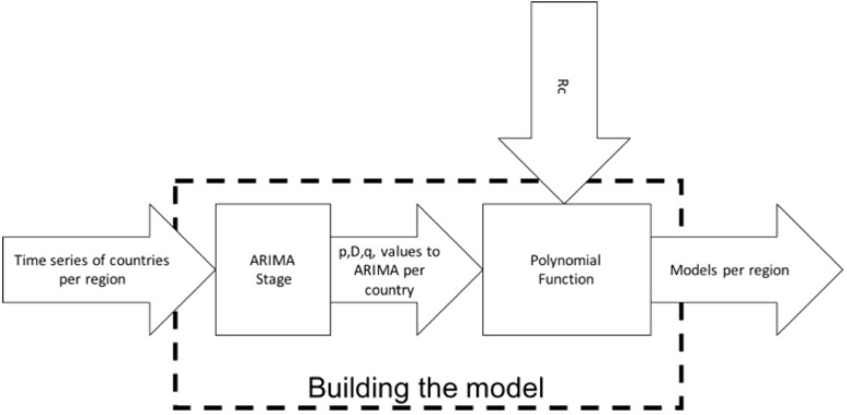
Fig. 2 shows a block diagram of this stage, which consists of the ARIMA and polynomial functions. The inputs of this stage are time series of the countries per region and Rc, which are explained in Section 3.1.1 (Arima Stage) and 3.1.2 (Polynomial Functions), respectively.
Fig. 2.
Block diagram of Building the model.
3.1.1. ARIMA stage
We use the time series “Total confirmed COVID-19 cases” per country. Then, we have a time series presented in the following equations:
| (1) |
| (2) |
In Eq. (1), y means the total confirmed cases per day presented in a country. In Eq. (2), means the day when each country detected the first COVID-19 patient. Then represents the number of days elapsed until April 25. For example, Canada detected the first patient on January 26. Then, we can rewrite Eq. (2) as shown Eq. (3).
| (3) |
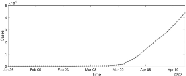
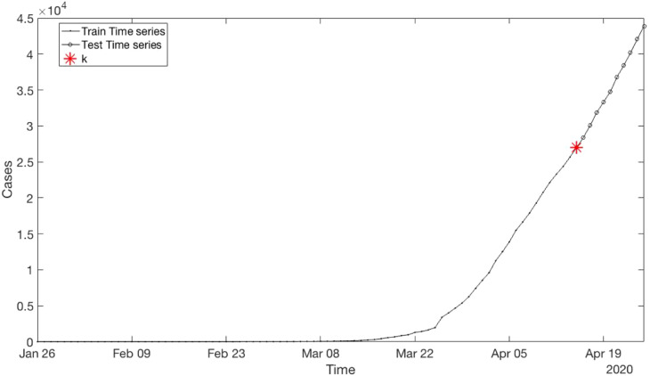
The Fig. 3 shows the time series of Canada. To compute the best parameters of ARIMA, the time series is separated into training time series and testing time series. To train time series is created using 90% of the data from the original time series. At the same time, test time series is created using 10% of the data from the original time series. The Fig. 4 shows the example using time series of Canada.
Fig. 3.
COVID-19 time series of Canada.
Fig. 4.
Canada time series separated into training and testing time series.
Then, we have two time series (Train and Test). The next equations presented in a formal way these time series.
| (4) |
| (5) |
| (6) |
| (7) |
| (8) |
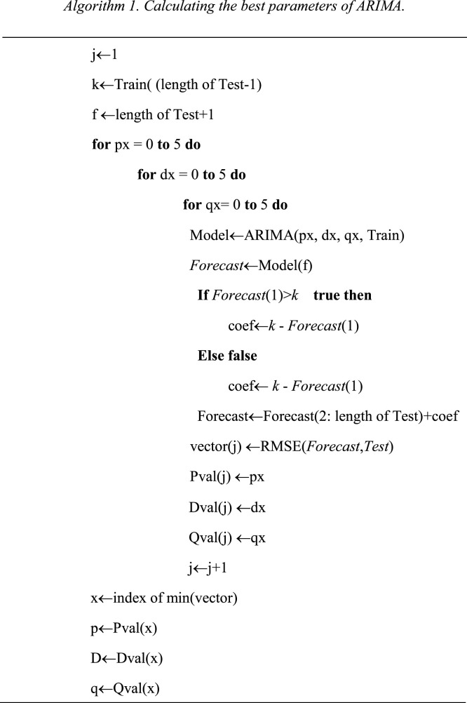
In Eq. (4), the k value is calculated, this value is the threshold to separate the data between Train and Test. Eqs. (5), (7) present the Train and the Test time series, respectively. Then, Algorithm 1 is applied to calculate the best parameters of an autoregressive integrated moving average (ARIMA).
ARIMA is a statistical analysis, it uses time series data. The ARIMA predicts future values by examining the differences between values in the time series. An ARIMA model consists of 3 components Auto regression (AR), Integrated (I), and Moving average (MA). Each component is a parameter. To represent these parameters, ARIMA models use a standard notation p, D, and q. This standard notation indicates the type of ARIMA model used. Where p means the number of lag observations, D means the degree of difference, and q means the order of the moving average, for further details refer to [14], [20], [21].
In the previous Algorithm, Root Mean Square Error (RMSE) [22] measures the stability between the original data and forecast data, RMSE is calculate using Eq. (9).
| (9) |
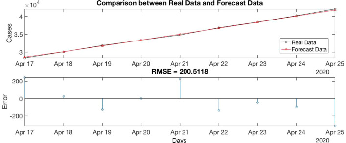
In our example, the algorithm 1 is applied into Train Canada Time series. Then, we have p, D, q values, p is 3, D is 2 and q is 4. Fig. 5 shows a comparison between the Real data (Test Time series) and Forecast Data of Canada.
Fig. 5.
Comparison between Real data and Forecast Data of Canada.
This process is applied to each country. Appendix A presents the p, D, q values of the ARIMA model and the RMSE to each analyzed country.
3.1.2. Polynomial functions
The ARIMA stage calculated the p, D, q values to each country. In this stage, we use these values, the information of cases confirmed COVID-19 per million people on April 25, and the Population per million people (ppMP). Table 1 shows an example of the obtained values in the previous stage, which are used in this stage.
Table 1.
Data of North America.
| Country | Population per million people (ppMp) | Total confirmed COVID-19 cases per 1M people |
ARIMA Parameters |
RMSE average 640.61 | |||
|---|---|---|---|---|---|---|---|
| April 25 | May-11 | p | D | q | |||
| Belize | 0.390 | 45.269 | 45.269 | 0 | 2 | 0 | 2.830E−07 |
| Canada | 37.411 | 1162.546 | 1824.167 | 3 | 2 | 3 | 2.611E+02 |
| Cuba | 11.333 | 113.450 | 155.916 | 5 | 1 | 3 | 2.128E+01 |
| Dominican Republic | 10.739 | 529.964 | 953.825 | 5 | 0 | 3 | 6.851E+01 |
| Grenada | 0.112 | 133.311 | 186.635 | 5 | 1 | 3 | 2.452E−01 |
| Guatemala | 17.581 | 24.001 | 58.720 | 2 | 2 | 5 | 1.671E+01 |
| Haiti | 11.263 | 6.314 | 15.961 | 3 | 3 | 1 | 2.392E+00 |
| Honduras | 9.746 | 59.669 | 199.099 | 4 | 3 | 1 | 1.719E+01 |
| Jamaica | 2.948 | 97.259 | 169.528 | 5 | 3 | 3 | 7.446E+00 |
| Mexico | 127.576 | 99.835 | 271.630 | 2 | 3 | 0 | 1.614E+02 |
| Nicaragua | 6.546 | 1.660 | 2.415 | 5 | 5 | 3 | 3.859E−01 |
| Panama | 4.246 | 1237.146 | 1957.927 | 3 | 1 | 5 | 2.141E+01 |
| United States | 329.065 | 2690.383 | 4017.488 | 4 | 1 | 3 | 7.750E+03 |
This stage calculates the polynomial function for ARIMA parameters (p, D, q). This fact means, we must calculate 3 polynomial functions, one for each ARIMA Parameter. Then, we create the Matrixes V , V , V , which have the p, D, q values for the countries in the region. Rc is a matrix, each one of the elements of Rc belongs to one country. These elements are calculated per country as follows: the numbers of confirmed COVID-19 cases on April 25 multiply per the population (ppMp).
| (10) |
| (11) |
| (12) |
| (13) |
| (14) |
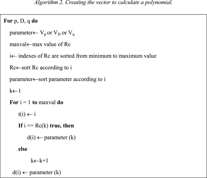
In our example k=1, 2, 3, …, 13. Then we need to apply the Algorithm 2 on V , V , V .
The Algorithm 2 creates the vectors t and d. The vector t starts in 1 and finishes in the maximum value of Rc. The vector d has the information of the ARIMA parameters. Then, we need to calculate a polynomial p(t) of degree n, that is the best fit for the data in the vector d, as shown Eq. (15).
| (15) |
| (16) |
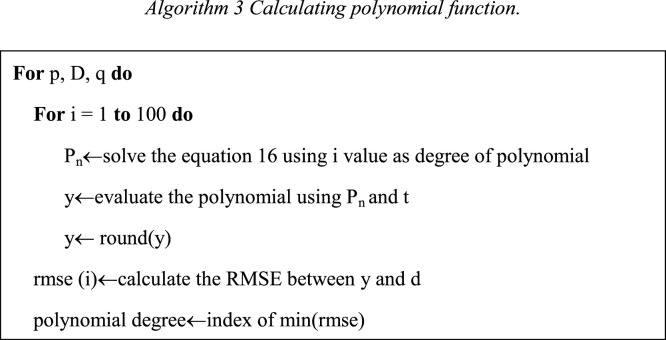
To solve Eq. (15), we present the problem as shown the Eq. (16). Then, t is used to form Vandermonde matrix [15] V with n+1 columns and m rows. Where m is the length of d. After to solve the Eq. (16), we find the values of , P 2,…, P . To calculate the best values of , we propose the Algorithm 3.
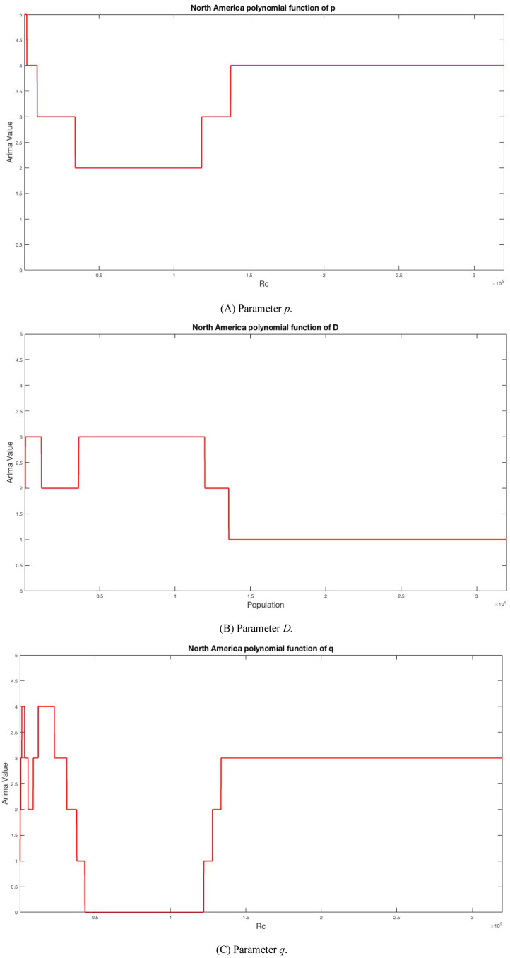
At the beginning of the Algorithms 2–3, we can take one of the ARIMA parameters, this fact means that the Algorithms 2 and 3 must be applicate 3 times, one time per ARIMA parameter. After the Algorithms 2 and 3 are applied the values to North America model are: 14 is degree of polynomial to parameter p, 15 is degree of polynomial to parameter D, and 47 is degree of polynomial to parameter q. The Eq. (18) shows an example of the polynomial created for ARIMA parameter D. Fig. 6 shows the polynomial functions for ARIMA parameters.
| (17) |
Fig. 6.
Polynomial Functions for North America Model.
The next Eqs. (18)–(20) show the polynomial functions for North America, the polynomials of all regions are available in Appendix B.
North America
| (18) |
| (19) |
| (20) |
3.2. Evaluating the model
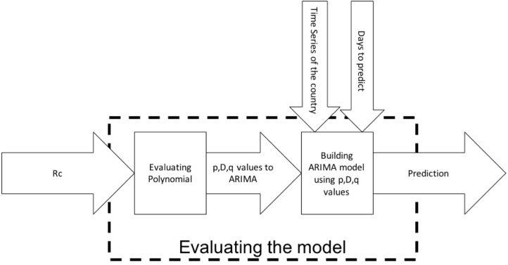
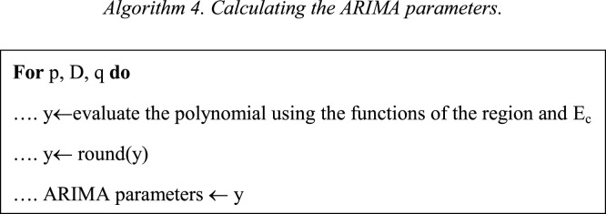
The Fig. 7 shows the block diagram of the Evaluating model stage. This stage has 3 inputs Ec, time series of the country until May 11, and days to predict. has the value of Total confirmed COVID-19 cases multiply per the population for the country to be evaluated in the region. In this evaluation, we use the data on May 11 and the polynomial functions creates in the previous stage. The Algorithm 4 is used to calculate the ARIMA parameters.
Fig. 7.
Block Diagram of Evaluating the model.
We apply the Algorithm 4 using the values of Canada on May 11 and the functions P(t), P(t), and P(t) Eqs. (18)-(20). Canada belongs to North America, so we use the functions of North America to calculate the ARIMA parameters. To calculate another country, we must use the functions which belong to the region of the country.
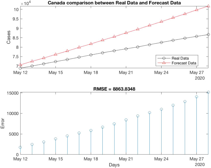
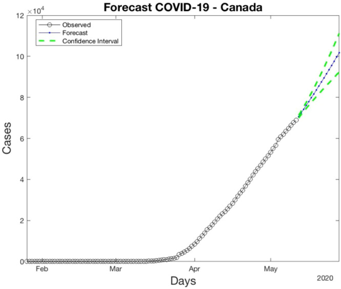
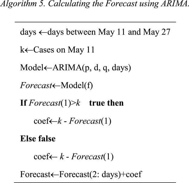
After we applied the Algorithm 4, the Canada ARIMA parameters are p=3, D=2, q=3. The next step is the prediction using the Algorithm 5. The Canada results using the model of North America are shown in Fig. 8, Fig. 9.
Fig. 8.
Comparison between Real Data and Forecast Data.
Fig. 9.
Forecasting of Canada.
The Eq. (9) is applied to calculate the RMSE between the forecast values and real values. Fig. 8 shows a comparison between the real and forecast signals and Fig. 9 shows the forecast of Canada with confidence interval of 95%.
4. Results
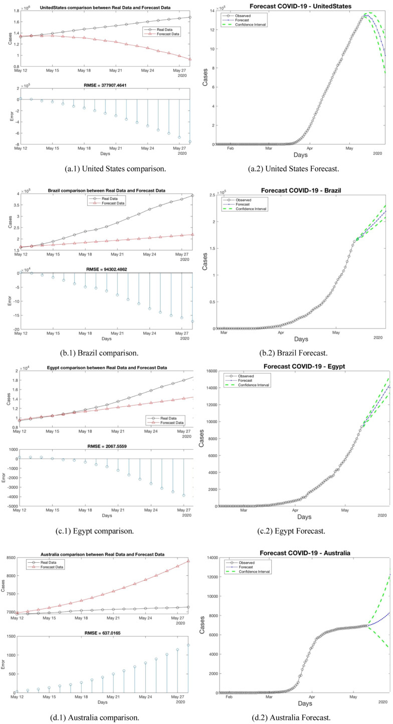
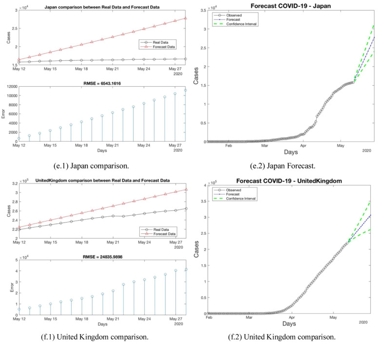
This section presents the results for each region analyzed. Table 2 shows the average RMSE per region. In the table, the RMSE is calculated between the forecast and the real values. Fig. 10 presents a comparison using RMSE and the forecast for one country per each region in the following way: (a) North America, (b) South America, (c) Africa, (d) Oceania, (e) Asia, and (f) Europe.
Table 2.
Average of RMSE results.
| Region | Average of RMSE between original and forecast signal in training stage | Average of RMSE between original and forecast signal from May 12 to May 27 |
|---|---|---|
| North America | 640.61 | 3.6051e+04 |
| South America | 104.78 | 2.0828e+04 |
| Africa | 13.80 | 1.4913e+03 |
| Oceania | 6.79 | 161.2570 |
| Asia | 89.46 | 3.52964e+03 |
| Europe | 218.59 | 2.88212e+04 |
| aAverage | 144.81 | 1.2723e+04 |
The average is calculated using the 145 countries.
Fig. 10.
An example of results per region. RMSE and Forecast (a) North America, (B) South America, (c) Africa, (d) Oceania, (e) Asia and (f) Europe.
5. Discussion
The Appendix A presents the results per country before to create the geographic models. These results belong to each country in the different regions. As we mention in Section 3.1.1, the time series are separated into modeling (90% of the signal) and testing (10% of the signal). Below, we will discuss each region in particular.
North America region has 13 countries; this region presents a RMSE average of 640.61. The RMSE average of this region is the most bigger between the regions. This fact appears, because the United States presents the most bigger RMSE between the 145 countries (7749.99), this country has the largest number of population in the region (329.06 ppMp). On the other hand, Belize presents the lowest RMSE. The United States has almost 96 times the population of Belize (0.39 ppMp).
Europe region consists of 33 countries. In this experiment, the countries, which present a ppMp major than 45 ppMp presents biggest RMSE. Spain presents an RMSE of 1892.33 with a 46.73 ppMp, Italy has 60.55 ppMp and presents an RMSE of 566.88, United Kingdom presents an RMSE of 728.13 with a 467.53 ppMp, Germany has 83.51 ppMp and presents an RMSE of 1075.02, and Russia presents an RMSE of 958.44 with a 145.87 ppMp. The RMSE average of this is 218.59.
Brazil presents a RMSE of 591, this country has the largest number of population in the region (211.04 ppMp). In contrast, Paraguay presents the lowest RMSE. Brazil has almost 30 times the population of Paraguay (7.05 ppMp). These countries belong to South America region, the RMSE average of this region is 104.78.
Asia region consists of 40 countries. In this region, Turkey presents the most bigger RMSE (696.35) with a population (83.43 ppMp). China and India have a ppMp major to one thousand, but the RMSE are 117.88 and 250.83, respectively. On the other hand, Yemen with a population less than 30 ppMp has a RMSE close to zero.
Egypt presents a RMSE of 84.08, this country has 110.38 ppMp. In contrast, Namibia presents a RMSE close to zero. Egypt has almost 41 times the population of Namibia (2.49 ppMp). These countries belong to Africa region, the RMSE average of this region is 13.8.
Oceania region consists of 4 countries. In this region, Australia presents the most bigger RMSE (24.76) with a population (25.20 ppMp). The lower RMSE is presented by Fiji with a population less than 1 ppMp.
For the regions North America, South America, Oceania, and Europe, there is a relation between the major ppMp and the error on the prediction. The RMSE of Africa is minor to 15, even though it has countries with 200 ppMp. This fact could be means a relation between the virus spread and the climate for example. For the region Asia the average RMSE is minor to 90, this area was the first area infected by COVID-19 so there are more available data in this area. Thus, we have more data to calculate the Forecast.
Table 3 shows a comparison between [10] and this work before to create the geographic models. As shown Table 3 this approach has better RMSE to forecast the virus in Italy, on the contrary [10] has better RMSE to predict the virus in Turkey and Spain. At first, it seems that their proposal is better than ours, but when the RMSE averages are compared, we can see that our proposal has a lower RMSE than them, besides we are analyzing 145 countries while they only analyze 3.
Table 3.
Comparison between [10] and this work.
| Country | RMSE |
|
|---|---|---|
| [10] | This work | |
| Italy | 1150.31 | 566.88 |
| Turkey | 138.35 | 1892.33 |
| Spain | 379.89 | 696.35 |
| Average | a556.183 | b144.81 |
Using 3 countries.
Using 145 countries.
Fig. 8 presents the results per one country in each region. In Fig. 8(a–f), we can see an upward trend in the number of cases, with the exception of the American States, which marks a decrease in the number of cases. Let us remember that from the beginning, the American States had the highest RMSE among all countries. When the geographic models are created, these models are used to predict new cases in a country. The results are shown in Table 2. The forecast is made 17 days after the models are calculated, we take this decision to have a real difference between the cases on April 25 and May 11 as shown the tables in Appendix A. As expected, the RMSE error grew because, the prediction is making 17 days after the models were created and we calculate 15 days of prediction cases. In these time interval, the actions as quarantine control, stay at home campaign, social distance taken by governments significantly affect the prediction. If the lector wants current predictions, the information needs to be updated and repeat the building the model stage.
Table A.1.
Data of the countries separated by geographical regions.
| North America | |||||||
| Country | Population per million people (ppMp) | Total confirmed COVID-19 cases per million people |
ARIMA parameters |
RMSE average 640.61 | |||
| April 25 | May-11 | p | D | q | |||
| Belize | 0.390351 | 45.269 | 45.269 | 0 | 2 | 0 | 0.000000283 |
| Canada | 37.411038 | 1162.546 | 1824.167 | 3 | 2 | 3 | 261.0992307 |
| Cuba | 11.333484 | 113.45 | 155.916 | 5 | 1 | 3 | 21.28255446 |
| Dominican Republic | 10.738957 | 529.964 | 953.825 | 5 | 0 | 3 | 68.51095035 |
| Grenada | 0.112002 | 133.311 | 186.635 | 5 | 1 | 3 | 0.245202091 |
| Guatemala | 17.581476 | 24.001 | 58.72 | 2 | 2 | 5 | 16.71287027 |
| Haiti | 11.263079 | 6.314 | 15.961 | 3 | 3 | 1 | 2.392474128 |
| Honduras | 9.746115 | 59.669 | 199.099 | 4 | 3 | 1 | 17.1948204 |
| Jamaica | 2.948277 | 97.259 | 169.528 | 5 | 3 | 3 | 7.44624079 |
| Mexico | 127.575529 | 99.835 | 271.63 | 2 | 3 | 0 | 161.3544175 |
| Nicaragua | 6.545503 | 1.66 | 2.415 | 5 | 5 | 3 | 0.385861038 |
| Panama | 4.24644 | 1237.146 | 1957.927 | 3 | 1 | 5 | 21.41200047 |
| United States | 329.064917 | 2690.383 | 4017.488 | 4 | 1 | 3 | 7749.995645 |
| South America | |||||||
| Country | Population per million people (ppMp) | Total confirmed COVID-19 cases per million people |
ARIMA parameters |
RMSE average 104.78 | |||
| April 25 | May-11 | p | D | q | |||
| Suriname | 0.581363 | 17.046 | 17.046 | 2 | 2 | 0 | 2.42E−09 |
| Uruguay | 3.461731 | 162.074 | 203.528 | 1 | 2 | 4 | 0.536253127 |
| Guyana | 0.782775 | 92.809 | 132.221 | 5 | 0 | 1 | 0.945527112 |
| Paraguay | 7.044639 | 31.265 | 99.965 | 4 | 3 | 1 | 3.977159335 |
| Venezuela | 28.515829 | 11.183 | 14.559 | 4 | 2 | 4 | 7.768192986 |
| Bolivia | 11.513102 | 69.134 | 218.966 | 5 | 5 | 4 | 13.19241251 |
| Chile | 18.952035 | 643.747 | 1510.027 | 5 | 3 | 4 | 31.85255857 |
| Argentina | 44.780675 | 75.737 | 127.8 | 2 | 1 | 2 | 34.307185 |
| Colombia | 50.339443 | 95.926 | 217.421 | 1 | 2 | 0 | 42.19486859 |
| Ecuador | 17.373657 | 633.847 | 1675.39 | 3 | 4 | 4 | 206.1259375 |
| Peru | 32.510462 | 656.56 | 2041.348 | 4 | 2 | 1 | 325.2189929 |
| Brazil | 211.049519 | 249.319 | 765.428 | 4 | 2 | 1 | 591.2483357 |
| Africa | |||||||
| Country | Population per million people (ppMp) | Total confirmed COVID-19 cases per million people |
ARIMA parameters |
RMSE average 13.80 | |||
| April 25 | May-11 | p | D | q | |||
| Namibia | 2.494524 | 6.297 | 6.297 | 4 | 2 | 0 | 3.38E−09 |
| Mauritania | 4.525698 | 1.505 | 1.721 | 1 | 2 | 0 | 1.88E−08 |
| Seychelles | 0.097741 | 111.857 | 111.857 | 0 | 3 | 0 | 0.00000302 |
| South Sudan | 11.062114 | 0.447 | 13.936 | 3 | 4 | 0 | 0.231695815 |
| Angola | 31.825299 | 0.761 | 1.369 | 2 | 0 | 1 | 0.272840126 |
| Madagascar | 26.969306 | 4.406 | 6.175 | 0 | 0 | 0 | 0.5 |
| Botswana | 2.303703 | 9.355 | 9.78 | 3 | 0 | 3 | 0.561333394 |
| Mauritius | 1.26967 | 260.268 | 261.054 | 5 | 2 | 0 | 0.577046983 |
| Togo | 8.082359 | 10.871 | 21.018 | 2 | 1 | 1 | 0.597788103 |
| Central African Republic | 4.745179 | 3.934 | 37.062 | 2 | 3 | 4 | 0.690491146 |
| Zimbabwe | 14.645473 | 1.951 | 2.422 | 4 | 1 | 4 | 0.920238223 |
| Eritrea | 3.497117 | 10.997 | 10.997 | 4 | 0 | 3 | 1.098426352 |
| Benin | 11.801151 | 4.784 | 26.313 | 1 | 1 | 5 | 1.123599466 |
| Chad | 15.946882 | 2.435 | 19.603 | 2 | 2 | 3 | 1.486804327 |
| Libya | 6.777453 | 8.878 | 9.314 | 5 | 1 | 0 | 1.802690408 |
| Zambia | 17.861034 | 4.569 | 14.524 | 4 | 1 | 5 | 2.264558145 |
| Ethiopia | 112.078727 | 1.018 | 2.079 | 3 | 0 | 3 | 2.448214102 |
| Burundi | 11.530577 | 1.009 | 1.598 | 1 | 4 | 4 | 2.535566664 |
| Cape Verde | 0.549936 | 158.277 | 442.456 | 4 | 2 | 2 | 2.574723428 |
| Burkina Faso | 20.321383 | 29.947 | 35.927 | 3 | 0 | 5 | 2.824155601 |
| Uganda | 44.269587 | 1.64 | 2.645 | 5 | 2 | 5 | 2.97488775 |
| Sierra Leone | 7.813207 | 10.28 | 38.486 | 3 | 3 | 1 | 3.214739643 |
| Liberia | 4.937374 | 23.133 | 39.346 | 4 | 1 | 5 | 3.84699105 |
| Niger | 23.310719 | 28.133 | 33.916 | 4 | 2 | 2 | 3.917381572 |
| Sudan | 42.813237 | 3.968 | 31.084 | 2 | 2 | 4 | 4.558386235 |
| Mali | 19.658023 | 16.049 | 34.764 | 3 | 2 | 2 | 5.436959696 |
| Kenya | 52.573967 | 6.249 | 12.497 | 5 | 2 | 2 | 5.646461767 |
| Mozambique | 30.366043 | 2.08 | 2.911 | 5 | 3 | 5 | 6.014669312 |
| Malawi | 18.628749 | 1.725 | 2.927 | 1 | 4 | 3 | 6.1920973 |
| Tunisia | 11.694721 | 78.013 | 87.32 | 1 | 0 | 0 | 8.775869024 |
| Gabon | 2.172578 | 77.278 | 296.981 | 4 | 3 | 2 | 11.10807476 |
| Nigeria | 200.963603 | 5.312 | 21.34 | 5 | 4 | 0 | 12.60385557 |
| Somalia | 15.442906 | 20.638 | 66.318 | 2 | 1 | 4 | 14.76084313 |
| Senegal | 16.296362 | 32.549 | 102.067 | 5 | 3 | 3 | 26.08610014 |
| Djibouti | 0.973557 | 1011.132 | 1224.694 | 1 | 1 | 3 | 26.43208425 |
| Cameroon | 25.876387 | 52.852 | 97.153 | 1 | 2 | 2 | 30.35431279 |
| Algeria | 43.053054 | 71.31 | 130.51 | 2 | 0 | 3 | 30.43462472 |
| Equatorial Guinea | 1.355982 | 151.106 | 312.904 | 1 | 2 | 1 | 41.34353663 |
| Ghana | 30.417858 | 41.161 | 137.193 | 5 | 2 | 2 | 47.53364114 |
| Guinea | 12.771246 | 72.643 | 163.408 | 3 | 5 | 0 | 59.82419028 |
| South Africa | 58.558267 | 71.153 | 168.862 | 3 | 3 | 5 | 65.82375285 |
| Morocco | 36.471766 | 101.814 | 164.262 | 1 | 1 | 0 | 70.07161038 |
| Egypt | 100.388076 | 39.987 | 91.856 | 5 | 1 | 3 | 84.08557986 |
| Oceania | |||||||
| Country | Population per million people (ppMp) | Total confirmed COVID-19 cases per million people |
ARIMA parameters |
RMSE average 6.79 | |||
| April 25 | May-11 | p | D | q | |||
| Fiji | 0.889955 | 20.079 | 20.079 | 0 | 2 | 0 | 0.000000105 |
| Papua New Guinea | 8.776119 | 0.894 | 0.894 | 3 | 2 | 2 | 0.321552716 |
| New Zealand | 4.783062 | 231.635 | 237.857 | 3 | 3 | 0 | 2.092622312 |
| Australia | 25.2032 | 262.237 | 272.197 | 1 | 3 | 1 | 24.7684965 |
| Asia | |||||||
| Country | Population per million people (ppMp) | Total confirmed COVID-19 cases per million people |
ARIMA parameters |
RMSE average 89.46 | |||
| April 25 | May-11 | p | D | q | |||
| Yemen | 29.161922 | 0.034 | 1.71 | 1 | 2 | 1 | 8.46E−16 |
| Laos | 7.169456 | 2.611 | 2.611 | 0 | 2 | 0 | 0.000000474 |
| Brunei | 0.433296 | 315.441 | 322.298 | 5 | 1 | 1 | 0.201374663 |
| Mongolia | 3.225166 | 10.981 | 12.812 | 5 | 3 | 2 | 0.42737412 |
| Bhutan | 0.763094 | 9.072 | 11.664 | 0 | 5 | 3 | 0.854706352 |
| Vietnam | 96.462108 | 2.774 | 2.959 | 0 | 0 | 0 | 0.894427191 |
| Syria | 17.070132 | 2.4 | 2.686 | 1 | 2 | 3 | 1.2290986 |
| Kyrgyzstan | 6.415851 | 101.928 | 155.728 | 4 | 3 | 1 | 1.764150638 |
| Myanmar | 54.045422 | 2.647 | 3.308 | 4 | 1 | 3 | 1.810985483 |
| Jordan | 10.101697 | 43.222 | 52.925 | 5 | 2 | 0 | 1.976423483 |
| Lebanon | 6.855709 | 101.971 | 123.802 | 3 | 0 | 2 | 3.248815136 |
| Nepal | 28.608715 | 1.682 | 4.119 | 3 | 2 | 4 | 4.05357834 |
| Georgia | 3.996762 | 111.301 | 159.181 | 0 | 1 | 4 | 4.895198267 |
| Maldives | 0.530957 | 236.799 | 1544.746 | 5 | 4 | 1 | 5.924589657 |
| Cyprus | 1.198574 | 917.914 | 1025.232 | 4 | 0 | 4 | 6.066194022 |
| Azerbaijan | 10.047719 | 157.015 | 248.442 | 4 | 0 | 5 | 11.83730777 |
| Thailand | 69.625581 | 40.888 | 43.195 | 3 | 0 | 0 | 12.58960875 |
| Iraq | 39.309789 | 42.464 | 68.792 | 1 | 3 | 3 | 15.52536699 |
| Uzbekistan | 32.981715 | 54.856 | 72.246 | 5 | 1 | 3 | 18.9777337 |
| Armenia | 2.957728 | 565.936 | 1118.035 | 0 | 3 | 4 | 19.92595139 |
| SriLanka | 21.323734 | 19.614 | 40.302 | 3 | 2 | 4 | 20.83410943 |
| Malaysia | 31.949789 | 175.833 | 205.648 | 2 | 1 | 5 | 27.80701783 |
| Kuwait | 4.207077 | 612.097 | 2034.392 | 0 | 2 | 2 | 44.83279931 |
| Oman | 4.974992 | 350.525 | 665.606 | 2 | 0 | 2 | 48.21943289 |
| Iran | 82.913893 | 1050.017 | 1281.096 | 5 | 3 | 0 | 50.19983585 |
| Afghanistan | 38.041757 | 34.705 | 113.08 | 5 | 2 | 0 | 75.99268382 |
| Bangladesh | 163.046173 | 28.472 | 88.998 | 5 | 3 | 0 | 79.01328851 |
| Qatar | 2.832071 | 2958.98 | 7816.568 | 1 | 2 | 0 | 97.6076415 |
| Bahrain | 1.641164 | 1479.799 | 2903.767 | 1 | 2 | 2 | 99.73990182 |
| Philippines | 108.116622 | 65.632 | 98.502 | 4 | 0 | 0 | 103.1445092 |
| Indonesia | 270.625567 | 30.019 | 51.301 | 5 | 1 | 5 | 110.4601355 |
| Israel | 8.519373 | 1739.695 | 1903.636 | 0 | 2 | 4 | 113.630396 |
| China | 1433.783692 | 58.291 | 58.368 | 5 | 0 | 0 | 117.8792989 |
| United Arab Emirates | 9.770526 | 938.385 | 1839.966 | 5 | 5 | 0 | 188.3682723 |
| Saudi Arabia | 34.268529 | 433.793 | 1121.622 | 3 | 3 | 2 | 226.4705085 |
| India | 1366.417756 | 17.758 | 48.661 | 5 | 2 | 3 | 250.833 |
| Pakistan | 216.565317 | 54.053 | 140.073 | 4 | 3 | 4 | 266.1868764 |
| Japan | 126.860299 | 101.932 | 124.909 | 1 | 1 | 2 | 399.4484529 |
| Singapore | 5.804343 | 1910.657 | 3988.826 | 1 | 2 | 2 | 449.3506577 |
| Turkey | 83.429607 | 1243.931 | 1644.042 | 5 | 3 | 3 | 696.3506539 |
| Europe | |||||||
| Country | Population per million people (ppMp) | Total confirmed COVID-19 cases per million people |
ARIMA parameters |
RMSE average 218.59 | |||
| April 25 | May-11 | p | D | q | |||
| Montenegro | 0.627988 | 507.912 | 515.873 | 2 | 2 | 0 | 0.988109524 |
| Malta | 0.440377 | 1012.368 | 1123.344 | 5 | 3 | 0 | 3.539156254 |
| Latvia | 1.90674 | 415.65 | 497.826 | 5 | 1 | 4 | 3.594220963 |
| Iceland | 0.339037 | 5242.491 | 5277.656 | 3 | 2 | 5 | 5.129808852 |
| Croatia | 4.130299 | 489.371 | 532.73 | 1 | 0 | 5 | 7.425098776 |
| Estonia | 1.325649 | 1209.915 | 1310.93 | 4 | 0 | 5 | 10.28679943 |
| Hungary | 9.68468 | 252.889 | 339.946 | 3 | 1 | 5 | 13.10475646 |
| Norway | 5.378859 | 1366.477 | 1493.938 | 5 | 2 | 1 | 14.35761421 |
| Slovakia | 5.457012 | 249.101 | 266.867 | 4 | 2 | 1 | 15.43096651 |
| Albania | 2.880913 | 235.597 | 301.619 | 5 | 2 | 4 | 15.44541938 |
| Lithuania | 2.759631 | 517.946 | 543.292 | 1 | 0 | 5 | 15.54234467 |
| Luxembourg | 0.61573 | 5902.782 | 6207.906 | 1 | 2 | 4 | 18.86761887 |
| Bulgaria | 7.000117 | 170.974 | 282.797 | 5 | 3 | 3 | 26.9764822 |
| Slovenia | 2.078654 | 660.435 | 700.841 | 4 | 2 | 5 | 29.45549614 |
| Czech Republic | 10.689213 | 679.15 | 758.522 | 5 | 1 | 4 | 32.36197356 |
| Austria | 8.955108 | 1673.033 | 1752.865 | 4 | 1 | 4 | 41.48747638 |
| Serbia | 8.772228 | 1099.698 | 1486.348 | 3 | 2 | 2 | 43.17539749 |
| Finland | 5.532159 | 793.218 | 1076.034 | 0 | 3 | 2 | 46.3725334 |
| Denmark | 5.771877 | 1417.423 | 1800.524 | 2 | 1 | 1 | 50.60316184 |
| Sweden | 10.036391 | 1739.433 | 2606.327 | 3 | 2 | 5 | 87.03004062 |
| Romania | 19.364558 | 541.489 | 798.537 | 4 | 2 | 5 | 102.4828358 |
| Poland | 37.887771 | 287.793 | 422.653 | 5 | 1 | 4 | 105.4066726 |
| Portugal | 10.226178 | 2282.207 | 2704.893 | 4 | 1 | 5 | 108.4530628 |
| Ukraine | 43.993643 | 185.783 | 348.289 | 2 | 5 | 2 | 159.7185476 |
| Ireland | 4.882498 | 3682.615 | 4657.139 | 1 | 4 | 2 | 172.2604087 |
| Belgium | 11.539326 | 3821.783 | 4580.048 | 5 | 2 | 0 | 207.3927744 |
| Belarus | 9.452409 | 928.426 | 2431.18 | 5 | 2 | 5 | 268.7103234 |
| Netherlands | 17.097123 | 2132.201 | 2487.734 | 5 | 0 | 0 | 387.229697 |
| Italy | 60.550092 | 3191.997 | 3623.278 | 4 | 3 | 3 | 566.8847446 |
| United Kingdom | 67.530161 | 2113.307 | 3228.692 | 2 | 1 | 0 | 728.1254615 |
| Russia | 145.87226 | 470.225 | 1436.864 | 5 | 5 | 1 | 958.4432358 |
| Germany | 83.517046 | 1819.418 | 2023.956 | 4 | 1 | 0 | 1075.024974 |
| Spain | 46.736782 | 4454.496 | 4871.587 | 0 | 1 | 0 | 1892.331932 |
6. Conclusion
We can conclude that the algorithm to model and evaluate the ARIMA models is able to develop models, which have low RMSE. On the other hand, this work shows a way to model the COVID spread started in particular cases to generate a general case. We can conclude, this work contributes to researchers working in COVID-19 prediction. It shows there is a relation between the virus spread and the different variables present in the countries, which belong to the same geographic region. Interestingly, we can find a show relation between the population in a country and RMSE error in a prediction. In future challenges of the proposed work different variables could be analyzed, for example, the date when the first coronavirus case is detected in the country, humidity, temperature, among other variables. Other kinds of clusters could be applied like cultural behavior, religious behavior, hygiene habits, feeding habits, among others. The approach is able to make current predictions, just the information needs to be updated.
Declaration of Competing Interest
The authors declare that they have no known competing financial interests or personal relationships that could have appeared to influence the work reported in this paper.
Acknowledgments
This study is supported by JSPS, Japan KAKENHI (Grants-in-Aid for Scientific Research) #JP20K11955.
Appendix A.
See Table A.1.
Appendix B.
North America
South America
Africa
Oceania
Asia
Europe
References
- 1.World Health Organization, Coronavirus disease (COVID-19) outbreak situation retrieved from: Online Resource.
- 2.Narin Ali, Kaya Ceren, Pamuk Ziynet. 2020. Automatic detection of coronavirus disease (COVID-19) using X-ray images and deep convolutional neural networks. arXiv, 003.10849. [DOI] [PMC free article] [PubMed] [Google Scholar]
- 3.Lin Chen, Ding Yuxiao, Xie Bin, Sun Zhujian, Li Xiaogang, Chen Zixian, Niu Meng. Asymptomatic novel coronavirus pneumonia patient outside Wuhan: The value of CT images in the course of the disease. Clin. Imaging. 2020;63:7–9. doi: 10.1016/j.clinimag.2020.02.008. [DOI] [PMC free article] [PubMed] [Google Scholar]
- 4.. BioSpace, Quotient Sciences and CytoAgents Accelerate Potential Treatment for COVID-19 Cytokine Storm, retrieved from: Online Resource.
- 5.Benvenuto Domenico, Giovanetti Marta, Vassallo Lazzaro, Angeletti Silvia, Ciccozzi Massimo. Data in Brief, Vol. 29. 2020. Application of the ARIMA model on the COVID-2019 epidemic dataset. (ISSN 2352-3409) [DOI] [PMC free article] [PubMed] [Google Scholar]
- 6.Simon Fong, Li Gloria, Dey Nilanjan, Gonzalez Crespo Ruben, Herrera-Viedma Enrique. Finding an accurate early forecasting model from small dataset: A case of 2019-nCoV novel coronavirus outbreak. Int. J. Interact. Multimed. Artif. Intell. 2020;6:132–140. doi: 10.9781/ijimai.2020.02.002. [DOI] [Google Scholar]
- 7.Perone Gaetano. 2020. An ARIMA model to forecast the spread and the final size of COVID-2019 epidemic in Italy. arXiv:2004.00382. [Google Scholar]
- 8.Guorong Ding, Xinru Li, Yang Shen, Brief Analysis of the ARIMA model on the COVID-19 in Italy, medRxiv 2020.04.08.20058636. 10.1101/2020.04.08.20058636. [DOI]
- 9.Tandon Hiteshi, Ranjan Prabhat, Chakraborty Tanmoy, Suhag Vandana. 2020. Coronavirus (COVID-19): ARIMA based time-series analysis to forecast near future. arXiv:2004.07859. [Google Scholar]
- 10.Lutfi Bayyurt, Burcu Bayyurt, Forecasting of COVID-19 Cases and Deaths Using ARIMA Models, medRxiv 2020.04.17.20069237. 10.1101/2020.04.17.20069237. [DOI]
- 11.Fong Simon James, Li Gloria, Dey Nilanjan, Crespo Rubén González, Herrera-Viedma Enrique. Composite Monte Carlo decision making under high uncertainty of novel coronavirus epidemic using hybridized deep learning and fuzzy rule induction. Appl. Soft Comput. 2020;93 doi: 10.1016/j.asoc.2020.106282. [DOI] [PMC free article] [PubMed] [Google Scholar]
- 12.Singh R.K., Rani M., Bhagavathula A.S., Sah R., Rodriguez-Morales A.J., Kalita H., Nanda C., Sharma S., Sharma Y.D., Rabaan A.A., Rahmani J., Kumar P. Prediction of the COVID-19 pandemic for the top 15 affected countries: Advanced autoregressive integrated moving average (ARIMA) model. JMIR Public Health Surv. 2020;6(2) doi: 10.2196/19115. [DOI] [PMC free article] [PubMed] [Google Scholar]
- 13.Duan Xingde, Zhang Xiaolei. ARIMA modelling and forecasting of irregularly patterned COVID-19 outbreaks using Japanese and South Korean data. 2020. (ISSN 2352-3409) [DOI] [PMC free article] [PubMed] [Google Scholar]
- 14.Bertozzi Andrea L., Franco Elisa, Mohler George, Short Martin B., Sledge Daniel. The challenges of modeling and forecasting the spread of COVID-19. Proc. Natl. Acad. Sci. 2020;117(29):16732–16738. doi: 10.1073/pnas.2006520117. [DOI] [PMC free article] [PubMed] [Google Scholar]
- 15.Li Lixiang, Yang Zihang, Dang Zhongkai, Meng Cui, Huang Jingze, Meng Haotian, Wang Deyu, Chen Guanhua, Zhang Jiaxuan, Peng Haipeng, Shao Yiming. Propagation analysis and prediction of the COVID-19. Infect. Dis. Model. 2020;5:282–292. doi: 10.1016/j.idm.2020.03.002. [DOI] [PMC free article] [PubMed] [Google Scholar]
- 16.Mizumoto Kenji, Chowell Gerardo. Transmission potential of the novel coronavirus (COVID-19) onboard the diamond Princess Cruises Ship. Infect. Dis. Model. 2020;5:264–270. doi: 10.1016/j.idm.2020.02.003. [DOI] [PMC free article] [PubMed] [Google Scholar]
- 17.Box G.E.P., Jenkins G.M. Forecasting and Control. Holden-Day; San Francisco: 1976. Time series analysis. [Google Scholar]
- 18.Max Roser A., Ritchie Hannah, Ortiz-Ospina Esteban, Hasell Joe. 2020. Coronavirus pandemic (COVID-19) Published online at OurWorldInData.org. Retrieved from: ’ https://ourworldindata.org/coronavirus’ [Online Resource] [Google Scholar]
- 19.United Nations, Department of Economic and Social Affairs, Population Dynamics, Retreived from: Online Resource.
- 20.Fattah J., Ezzine L., Aman Z., El Moussami H., Lachhab A. Forecasting of demand using ARIMA model. Int. J. Eng. Bus. Manag. 2018;10 [Google Scholar]
- 21.Ho S.L., Xie M. The use of ARIMA models for reliability forecasting and analysis. Comput. Ind. Eng. 1998;35(1–2):213–216. doi: 10.1016/S0360-8352(98)00066-7. [DOI] [Google Scholar]
- 22.Serrà J., Arcos J.L. An empirical evaluation of similarity measures for time series classification. Knowl. Based Syst. 2014;67:305–314. [Google Scholar]


