EMKLAS: A New Automatic Scoring System for Early and Mild Keratoconus Detection

Abstract

Purpose

Create a unique predictive model based on a set of demographic, optical, and geometric variables with two objectives: classifying keratoconus (KC) in its first clinical manifestation stages and establishing the probability of having correctly classified each case.

Methods

We selected 178 eyes of 178 subjects (115 males; 64.6%; 63 females, 35.4%). Of these, 74 were healthy control subjects, and 104 suffered from KC according to the RETICS grading system (61 early KC, 43 mild KC). Only one eye from each patient was selected, and 27 different parameters were studied (demographic, clinical, pachymetric, and geometric). The data obtained were used in an ordinal logistic regression model programmed as a web application capable of using new patient data for real-time predictions.

Results

EMKLAS, an early and mild KC classifier, showed good training performance figures, with 73% global accuracy and a 95% confidence interval of 65% to 79%. This classifier is particularly accurate when validated by an independent sample for the control (79%) and mild KC (80%) groups. The accuracy of the early KC group was remarkably lower (69%). The variables included in the model were age, gender, corrected distance visual acuity, 8-mm corneal diameter, and posterior minimum thickness point deviation.

Conclusions

Our web application allows fast, objective, and quantitative assessment of early and mild KC in detection and classification terms and assists ophthalmology professionals in diagnosing this disease.

Translational Relevance

No single gold standard exists for detecting and classifying preclinical KC, but the use of our web application and EMKLAS score may aid the decision-making process of doctors.

Introduction

Keratoconus (KC) is a progressive corneal ectasia that manifests as a cone-like bulge and reduced corneal thickness.¹ Diagnosing KC in its milder forms can be achieved based on clinical evidence and corneal tomography analysis.² However, in its more incipient phases, when patients are asymptomatic,^3,4 KC detection remains a clinical challenge.

Given the unpredictable character of this disease,⁴ it is vitally important to correctly identify patients suffering postsurgical iatrogenic ectasia,^5–11 as several studies suggest that 2.6% of the patients planning to undergo refractive surgery are suspected of suffering KC.¹²

An increasing number of technologies allow researchers to combine various metrics to develop algorithms for use in ophthalmology,¹³ such as detecting KC in its early stages.^4,8 The application of these technologies, however, can produce significantly different results, particularly with regard to detecting KC, as no clear consensus has been reached on the relative importance of indices on which such algorithms are based and there are discrepancies in the criteria used to assess the risk probability associated with the disease developing. As a result, a practical multifactor formula capable of discriminating between incipient KC and normal eyes is very much needed.

Cavas-Martínez et al.^14,15 recently presented an innovative, virtual three-dimensional (3D) model of the cornea that registers the geometrical decompensation present during asymmetric disease progression. This model allows continuous and discreet analysis, based on morpho-geometrical variables, of the biomechanical instability related to collagen fiber orientation in the corneal matrix that is present with KC.

Different disease progression classifications for KC exist and are based on several indices¹⁶; however, processing the profuse information available can sometimes complicate optical-geometric evaluations. From an optical point of view, patients show deteriorated spectacle-corrected visual acuity during disease development; that is, their visual performance worsens as the degree of KC severity progresses. Based on this progression, a KC stages classification has been developed that is known as RETICS grading.^17,18

The purpose of this study was to develop a unique predictive model based on a set of demographic, optical, and geometric variables to classify KC in its first clinical manifestation stages and to establish the probability of correction after classifying each case.

Materials and Methods

Patients

For this observational comparative study, 178 eyes of 178 subjects between the ages of 15 and 76 years were selected; 115 of the subjects were male (64.6%) and 63 were female (35.4%). Of these, 74 were included in the healthy control group. Their ages ranged from 18 to 63 years (average age, 41 ± 23.7 years), and there were 42 males (56.7%) and 32 females (43.3%). The remaining 104 subjects had been diagnosed with KC; they were 16 to 76 years old, with 73 males (70.1%) and 31 females (29.9%). This second group was divided again into two subgroups depending on the degree of KC according to the RETICS grading system: I (early KC) or II (mild KC).¹⁸ The early KC group was comprised of 61 subjects ranging in age from 15 to 59 years (average age, 36.0 ± 21.0 years), of whom 45 were male (73.8%) and 16 female (26.2%). The mild KC group was comprised of 43 subjects ranging in age from 17 to 76 years old (average age, 46.2 ± 29.2 years), with 28 males (65.1%) and 15 females (34.9%).

A second dataset was obtained 4 months after recruiting the first set of individuals used for the training process, taking care to include no patient from the training group in the validation group. This new dataset represented 41 individuals, of whom 19 were healthy, 14 were classified as RETICS grade I, and eight were classified as RETICS grade II. This dataset was used to make an independent validation of the ordinal logistic regression model.

All of the subjects were recruited at Vissum Corporation Alicante (an institution affiliated with Miguel Hernández University, Elche, Spain) and formed part of the official Iberia database of KC cases generated for the National Network for Clinical Research in Ophthalmology RETICS-OFTARED. All of the participants provided written informed consent, and the study, which followed the tenets of the Declaration of Helsinki, was approved by the clinic's Ethics Committee for Clinical Research.

To avoid undesired biases, any subjects who had undergone previous ocular surgery, had worn contact lenses in the 4-week period running up to the tomographical evaluation, or showed any other ocular comorbidity that could affect the study outcomes were eliminated.

The cases in the control group were randomly selected from candidates for the refractive procedure, and the data included in the study were acquired during the patients’ presurgical consultations, always by the same experienced technician.

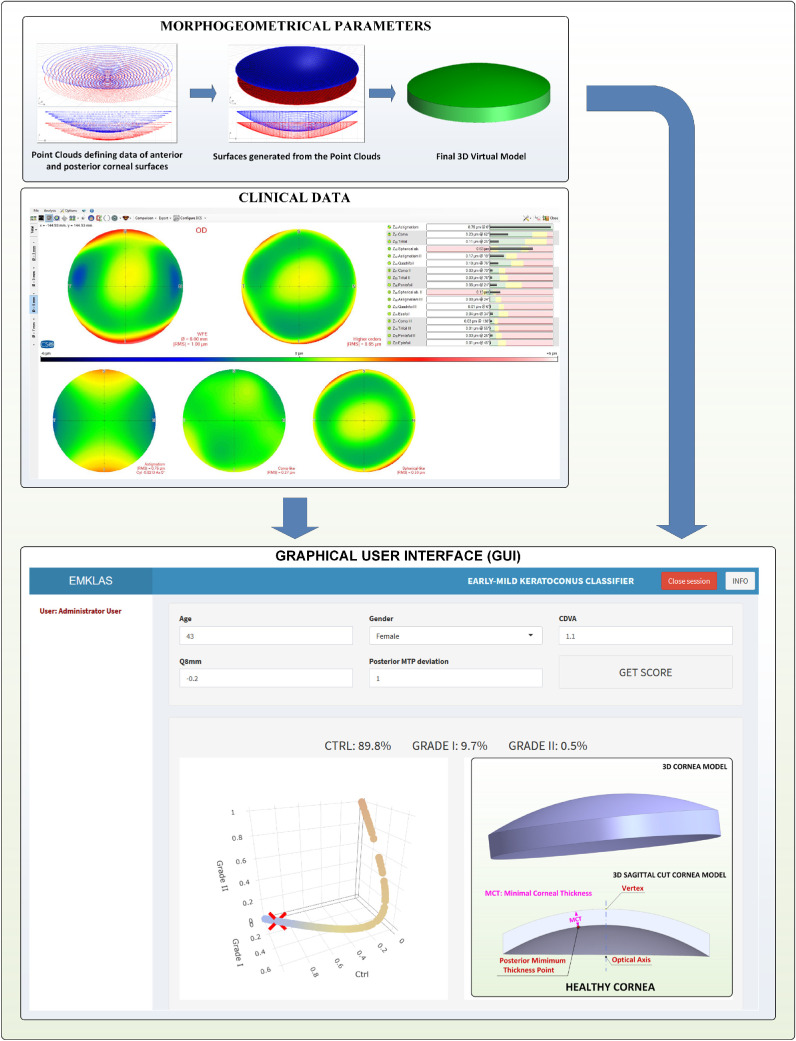
The procedure followed for both KC group diagnosis and classification was based on state-of-the-art clinical and topographical evaluations (Fig. 1), including ultrasonic pachymetry, fundus evaluation, manifest refraction (sphere and cylinder), slit-lamp biomicroscopy, uncorrected distance visual acuity (UDVA), corrected distance visual acuity (CDVA), and Goldmann tonometry.¹⁹ For all cases, clinicians searched for presurgical evidence of KC, such as the presence of the asymmetric bowtie pattern (with or without skewed axes), Fleischer's ring, Rizzuti's sign, Munson's sign, anterior stromal scar, or stromal thinning.

Figure 1.

Methodology proposed for generating the early and mild KC classifier.

Examination

All of the subjects were evaluated by Sirius tomography (Costruzione Strumenti Oftalmici, Florence, Italy) following the validated methodology guidelines previously created by our research group and which have been thoroughly described in earlier reports.^14,15 This methodology has proved its effectiveness in diagnosing¹⁵ and characterizing KC¹⁴ and is performed in two stages: 3D virtual modeling followed by morpho-geometric analysis.

3D Modeling

The outcome of this procedure is a personalized 3D corneal model that can be examined to determine morpho-geometric variables that have already been defined and utilized in previous studies.^14,15 Among these variables, posterior minimum thickness point deviation was selected for use in this study, along with the demographic and clinical parameters (Fig. 1).

Statistical Analysis

Exploratory and Descriptive Data Analysis

Quantitative variables were summarized by median ± interquartile range (IQR) and mean ± SD, and qualitative variables by count and percentage. Normality was tested by the Shapiro–Wilk test, and collinearity was measured with the Pearson correlation coefficient. The association between each quantitative variable and group (healthy individuals, early KC, or mild KC) was evaluated by the Kruskal–Wallis test, as most did not pass the normality test. A χ² test was used for the qualitative variable of gender. P < 0.05 was considered to be statistically significant.

Model Training and Fine-Tuning

The ordinal logistic regression technique was used to model the multivariate relation among all of the available parameters and grades:

$$\begin{array}{c}\hfill \log \frac{P\left(Y\le j\right)}{P(Y>j)}={\beta }_{j0}-{\beta }_1{x}_1-...-{\beta }_p{x}_p\end{array}$$ (1)

where Y is an ordinal outcome with J categories; P(Y ≤ j) is the cumulative probability of Y being less than or equal to a specific category J = 1, …, J – 1; β_j0 is the intercept for category j; and β₁, β₂, …, β_p are the coefficients for each predictor p20. It was assumed that the intercepts differed for each category, but slopes were constant across categories (proportional odds model). A backward procedure with the Akaike information criterion (AIC) was used to obtain a minimal set of variables containing the largest possible amount of information. Initially, a full model with all of the available parameters was created, and each parameter was then removed one by one to establish a new model. The AIC values for all of these models were calculated as²¹

$$\begin{array}{ccc}\hfill AIC& =& -2·\mathrm{maximized}\log -\mathrm{likelihood}\hfill \\ & & +2·\mathrm{number}\mathrm{of}\mathrm{parameters}\hfill \end{array}$$ (2)

The parameter that produced the most marked reduction in the AIC was removed, and the process was repeated until no further reduction in the AIC took place. The proportional odds assumption of the model was tested by the Venables and Ripley likelihood ratio test and by the Brant test.

Model goodness of fit was assessed using the Hosmer–Lemeshow test adapted for ordinal logistic regression to examine whether the observed proportions of events were similar to the predicted probabilities of occurrence in subgroups of the dataset using a χ² test. The McFadden pseudo-R² value was also calculated, defined as follows:

$$\begin{array}{c}\hfill pseudoR2=1-\frac{\ln \left(fittedmodel\right)}{\ln \left(nullmodel\right)}\end{array}$$

where ln indicates the log likelihood value and the null model has only an intercept as predictor.

Model Validation

The model was evaluated using accuracy, sensitivity, and specificity scores derived from the corresponding confusion matrix. An internal cross-validation procedure using bootstrap aggregating (bagging) was used.²² First, a new dataset was generated by sampling with replacement from the original dataset, which was the same size. Then, a new model was trained with these data and was later used to make predictions on the cases not included during training. This procedure was repeated 100 times to obtain a set of quality parameters that could be averaged. Confidence intervals were calculated. On average, 63.2% of the original data were used in all 100 training steps, with the remaining 36.8% being employed for validation purposes.

Then a second dataset of 41 patients was obtained 4 months after recruiting the first set of individuals and was used to make an independent validation of the ordinal logistic regression model.

Programs and Libraries

All of the statistical calculations were carried out by R v3.6.1 (R Foundation for Statistical Computing, Vienna, Austria),²³ and P < 0.05 was considered statistically significant. The packages dplyr, corrplot, nnet, MASS, generalhoslem, pscl, brant, effects, grid, caret, yarrr, and ROCR were used for the data preprocessing, analysis, and plotting, as well as for model calculation and validation. The Shiny (RStudio, Inc., Boston, MA)²⁴ and ShinyAuthr (Paul Campbell, Paris, France)²⁵ packages were utilized for web application development and deployment and for user authentication.

Statistical power analysis was conducted by simulation with the Wald test to estimate the power for each covariate according to sample size, as the literature describes.^26,27

Results

Of all the eyes considered, 41.5% were in the control group (74 healthy eyes), 34.3% were in the early KC group (61 eyes), and 24.2% were in the mild KC group (43 eyes). Table 1 summarizes all of the variables measured initially for all of the patients, who were then segregated into healthy individuals (control), patients showing early KC eyes, and those with a mild form of disease development. Some trends of the association between variables and grades were observed and were further tested by the Kruskal–Wallis test for the quantitative variables and the χ² test for the qualitative variable of gender. All of the quantitative variables except for age, axis, and spherical aberration (Z40) showed a significant relation, whereas no significant difference was found for gender. A non-parametrical test was used because most quantitative variables did not pass the normality test.

Table 1.

Demographic, Clinical, and Morphogeometric Parameters Segregated into Healthy (Control) and Early KC and Mild KC Patients

	Median ± IQR; Mean ± SD
	Total	Healthy	Early KC	Mild KC	P	P
	(N = 178)	(n = 74)	(n = 61)	(n = 43)	Normality	Association
Age (y)	38.0 ± 22.3; 39.6 ± 16.2	41.0 ± 23.7; 37.5 ± 14.9	36.0 ± 21.0; 40.5 ± 15.5	46.2 ± 29.2; 44.8 ± 19.2	< 0.001	0.208
Male; femalea	63 (35.4); 115 (64.6)	32 (43.2); 42 (56.8)	16 (26.2); 45 (73.8)	15 (34.9); 28 (65.1)	—	0.120
Sphere	–0.51 ± 3.50; –1.82 ± 4.30	0.00 ± 3.56; –0.86 ± 3.51	-0.08 ± 2.01; –0.81 ± 2.38	–1.00 ± 3.13; –2.53 ± 3.67	< 0.001	0.018
Cylinder	–1.88 ± 2.50; –2.02 ± 1.91	–0.50 ± 1.00; –0.65 ± 0.86	–2.25 ± 2.14; –2.24 ± 1.60	–2.63 ± 1.64; –2.95 ± 1.29	< 0.001	< 0.001
Axis	75.8 ± 81.1; 74.9 ± 55.3	80.1 ± 88.7; 66.8 ± 60.7	85.0 ± 65.0; 83.3 ± 50.9	75.8 ± 60.8; 84.4 ± 48.5	< 0.001	0.117
CDVA	0.94 ± 0.37; 0.80 ± 0.29	1.00 ± 0.00; 1.01 ± 0.05	0.96 ± 0.09; 0.95 ± 0.11	0.72 ± 0.19; 0.74 ± 0.11	< 0.001	< 0.001
PIO	12.0 ± 4.0; 13.3 ± 2.8	15.9 ± 3.6; 15.6 ± 2.8	11.5 ± 1.0; 11.7 ± 1.7	12.8 ± 3.0; 13.1 ± 2.0	< 0.001	< 0.001
Total RMS	2.39 ± 2.88; 3.02 ± 2.79	0.81 ± 0.55; 0.94 ± 0.69	2.39 ± 1.58; 2.55 ± 1.32	3.38 ± 1.38; 3.62 ± 1.65	< 0.001	< 0.001
High-order	1.12 ± 1.96; 1.88 ± 2.09	0.41 ± 0.14; 0.41 ± 0.11	1.42 ± 1.18; 1.46 ± 0.78	2.04 ± 0.50; 2.17 ± 0.86	< 0.001	< 0.001
Astigmatism	1.59 ± 2.14; 2.18 ± 2.06	0.69 ± 0.65; 0.79 ± 0.74	1.61 ± 1.73; 1.94 ± 1.32	2.26 ± 1.41; 2.77 ± 1.67	< 0.001	< 0.001
Coma Z31	0.74 ± 1.78; 1.54 ± 1.89	0.25 ± 0.12; 0.27 ± 0.12	0.77 ± 1.16; 1.09 ± 0.72	1.66 ± 0.71; 1.86 ± 0.84	< 0.001	< 0.001
Spherical aberration (Z40)	0.19 ± 0.32; 0.01 ± 0.76	0.21 ± 0.08; 0.22 ± 0.06	0.21 ± 0.34; 0.14 ± 0.32	0.10 ± 0.44; 0.09 ± 0.24	< 0.001	0.161
Coma-like	1.05 ± 1.98; 1.72 ± 1.94	0.32 ± 0.16; 0.32 ± 0.12	1.29 ± 1.20; 1.33 ± 0.76	1.93 ± 0.57; 2.06 ± 0.83	< 0.001	< 0.001
Spherical-like	0.43 ± 0.47; 0.64 ± 0.82	0.22 ± 0.08; 0.23 ± 0.05	0.49 ± 0.34; 0.55 ± 0.30	0.61 ± 0.34; 0.59 ± 0.27	< 0.001	< 0.001
Q8mm	–0.48 ± 0.81; –0.61 ± 0.65	–0.26 ± 0.21; –0.27 ± 0.19	–0.43 ± 0.76; –0.44 ± 0.62	–0.74 ± 0.79; –0.71 ± 0.47	< 0.001	< 0.001
Central thickness	507 ± 73; 499 ± 58	547 ± 46; 545 ± 31	500 ± 48; 499 ± 34	468 ± 51; 480 ± 34	0.081	< 0.001
Temporal	543 ± 65; 544 ± 48	585 ± 43; 578 ± 32	534 ± 58; 351 ± 38	515 ± 51; 524 ± 34	0.188	< 0.001
Nasal	577 ± 65; 579 ± 45	617 ± 50; 612 ± 36	566 ± 61; 563 ± 39	562 ± 34; 568 ± 37	0.709	< 0.001
Superior	588 ± 72; 589 ± 48	632 ± 42; 625 ± 36	585 ± 59; 574 ± 42	560 ± 39; 573 ± 32	0.031	< 0.001
Inferior	560 ± 60; 559 ± 53	597 ± 51; 596 ± 34	553 ± 63; 543 ± 41	553 ± 29; 547 ± 33	0.265	< 0.001
Volume	24.4 ± 2.7; 24.7 ± 1.9	26.2 ± 2.1; 25.9 ± 1.5	23.9 ± 1.17; 24.1 ± 1.46	23.5 ± 1.6; 23.9 ± 1.2	0.069	< 0.001
Anterior area	43.2 ± 0.4; 43.2 ± 0.5	43.1 ± 0.2; 43.1 ± 0.1	43.3 ± 0.3; 43.3 ± 0.2	43.3 ± 0.2; 43.3 ± 0.2	0.005	< 0.001
Posterior area	44.5 ± 0.6; 44.7 ± 0.8	44.3 ± 0.3; 44.3 ± 0.3	44.6 ± 0.5; 44.5 ± 0.3	44.7 ± 0.5; 44.7 ± 0.3	0.063	< 0.001
Anterior apex deviation	7.4e-5 ± 6.5e-3; 7.4e-3 ± 1.4e-2	0.0 ± 0.0; 2.7e-4 ± 8.8e-4	2.4e-4 ± 3.2e-3; 3.3e-3 ± 6.5e-3	2.3e-3 ± 1.2e-2; 8.1e-3 ± 0.1e-2	< 0.001	< 0.001
Posterior apex deviation	0.12 ± 0.12; 0.15 ± 0.09	0.07 ± 0.03; 0.07 ± 0.02	0.14 ± 0.09; 0.16 ± 0.08	0.17 ± 0.11; 0.19 ± 0.08	< 0.001	< 0.001
Anterior minimal thickness point deviation	0.90 ± 0.38; 0.95 ± 0.36	0.83 ± 0.30; 0.86 ± 0.30	0.97 ± 0.41; 1.01 ± 0.39	1.01 ± 0.52; 1.05 ± 0.34	< 0.001	0.003
Posterior minimal thickness point deviation	0.83 ± 0.35; 0.87 ± 0.33	0.77 ± 0.27; 0.80 ± 0.28	0.88 ± 0.37; 0.94 ± 0.36	0.92 ± 0.47; 0.98 ± 0.32	< 0.001	0.002

The corresponding P values for a Kruskal–Wallis univariate association test for each variable between groups are also shown.

^aGender is shown as n (%).

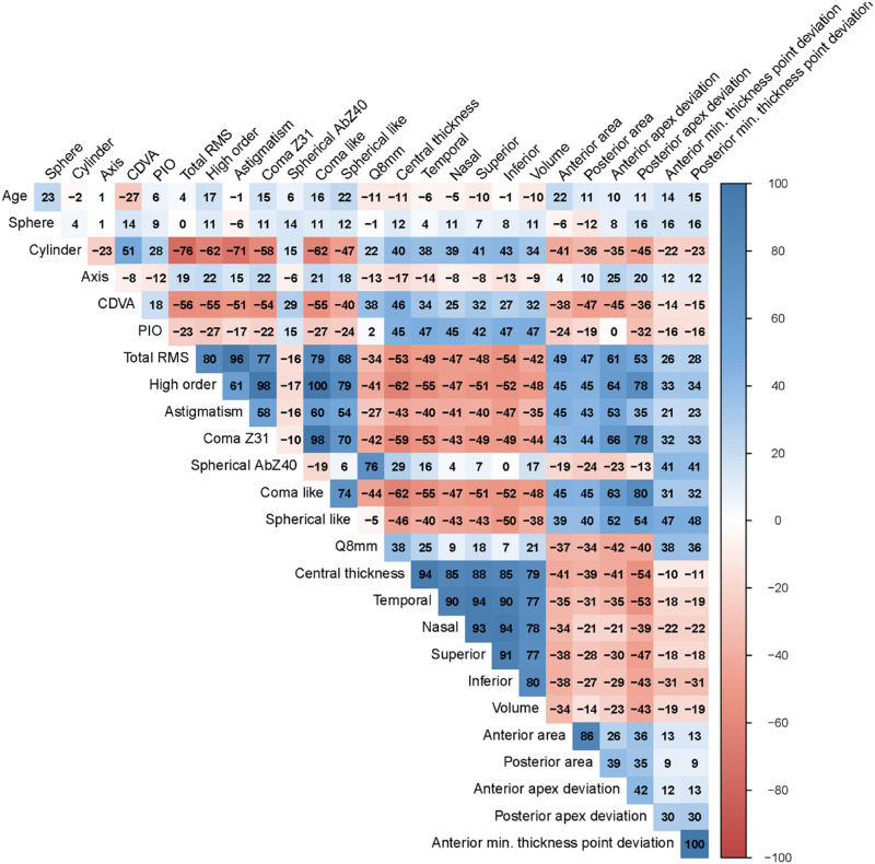
Figure 2 reveals that all of the variables, except for age, sphere, axis, spherical aberration (Z40), and anterior/posterior minimal thickness point deviations, were strongly correlated and, therefore, provided very little information. This finding suggested that a simple model with a limited amount of variables should be used when applying the ordinal logistic regression technique with a variable selection algorithm. A minimum set of predictors providing the most information was selected by a backward stepwise procedure using the AIC. The final model included the variables shown in Table 2, such as age and gender. When assessing the goodness of fit of this final model, the likelihood ratio test gave a P < 0.001, and P < 0.001 was also obtained by the Hosmer–Lemeshow test. The McFadden pseudo-R² gave a value of 0.507, indicating good predictive power.

Figure 2.

Correlation plot for quantitative variables. Color indicates a positive or negative correlation.

Table 2.

Ordinal Logistic Regression Model Summary

	Coefficient	Standard Error	t	P	Odds Ratio (95% CI)
Age	–0.009	0.011	–0.834	0.404	0.099 (0.970–1.013)
Gender	0.361	0.350	1.033	0.302	1.435 (0.073–2.872)
CDVA	–15.059	2.150	–7.005	<0.001	2.88e-7 (3.02e-9–1.47e-5)
Q8mm	–1.491	0.444	–3.360	0.001	0.225 (0.091–0.523)
Posterior minimum thickness point deviation	2.511	0.663	3.787	<0.001	12.32 (3.59–48.52)

Table shows the remaining variables after applying a backward stepwise procedure using the Akaike information criterion.

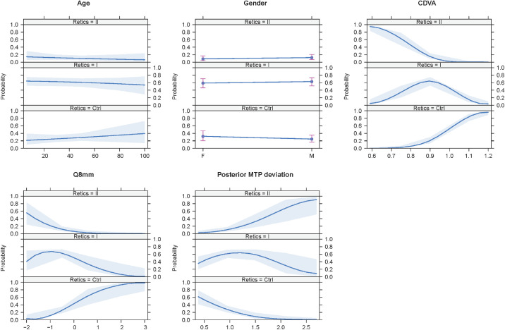
Figure 3 shows the effects plot for the included variables. Age and gender contributed very little, but CDVA, 8-mm corneal diameter (Q_8mm), and posterior minimum thickness point deviation made an important and apparently homogeneous contribution among the groups.

Figure 3.

Effects plot of the variables included in the ordinal logistic regression model. Age and gender made a very small contribution, whereas BCAV, Q_8mm, and posterior minimum thickness point deviation made an important and homogeneous contribution among the groups.

The model passed all of the tests run to check for the proportional odds assumption required for the ordinal logistic regression to be valid. The Venables and Ripley test value was 0.180, and the omnibus Brant test value was 0.250. The individual Brant test results for age, gender, CDVA, Q_8mm, and posterior minimum thickness point deviation were 0.307, 0.164, 0.196, 0.393, and 0.575, respectively. Thus, no significant deviation from assumptions was present.

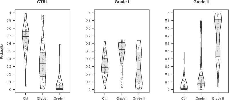
Figure 4 shows the distribution of scores for each group. The prediction score for the control group follows a markedly different distribution for the true control versus true early KC and mild KC individuals. A similar behavior was observed for the mild KC prediction score for true mild KC versus true control and early KC patients. Nonetheless, an early KC prediction score for the true early KC versus true control and mild KC patients does not show such marked differences and indicates that the early KC patients lie somewhere in a zone between the other two groups.

Figure 4.

Distribution of the scores generated by the ordinal logistic regression model over all of the training set individuals. Each plot corresponds to the predicted group score, and each bean in a plot corresponds to a reference group. Beans show approximate distribution, and boxes indicate median and 25th and 75th quartiles. Each point corresponds to a patient.

Table 3 shows the corresponding model confusion matrix, where similar results are observed.

Table 3.

Training Confusion Matrix Corresponding to the Ordinal Logistic Regression Model

Predicted	Control	Early KC	Mild KC
Control	63	18	1
Early KC	10	35	11
Mild KC	1	8	31

Table 4 reflects that the balanced accuracy for the control, early KC, and mild KC patients (0.83, 0.70, and 0.83, respectively), with an overall accuracy of 0.73 (95% confidence interval [CI], 0.65–0.79). McNemar's test yielded a P value of 0.430, indicating homogeneity of the results. Only one true mild KC patient was predicted to be a control patient, and, once again, only one true control patient was predicted to be a mild KC patient. A higher degree of misclassifying was present among the adjacent groups (control vs. early KC, or early KC vs. mild KC), with 47 of the patients (26.4%) being incorrectly classified by combining false-positives and false-negatives.

Table 4.

Ordinal Logistic Regression Model Training

	Control	Early KC	Mild KC
Sensitivity	0.85	0.57	0.72
Specificity	0.82	0.82	0.93
Balanced accuracy	0.83	0.70	0.83

Overall accuracy was 73% (95% CI, 65–79). McNemar's test indicated homogeneous results (P = 0.430).

Table 5 provides the inner validation procedure results, where 100 bootstrap resamples with substitution were obtained that contained the same total number of cases as the original dataset (n = 178). For each one, an equivalent ordinal logistic regression model was fitted using the same parameters indicated in Table 2. This fitted model was used to classify the remaining cases, which were those not used in the bootstrap sample. The quality measurements of the model for sensitivity and specificity terms were averaged from these results with their corresponding confidence intervals. We can observe that approximately similar results were obtained, with a slight trade-off between sensitivity and specificity but with significantly higher values for the control and mild KC prediction scores than for early KC.

Table 5.

Inner Validation Scores Obtained Using 100 Bootstrap Samples

	Control	Early KC	Mild KC
Area under the curve	0.87 ± 0.04	0.69 ± 0.06	0.94 ± 0.03
Sensitivity	0.91 ± 0.06	0.63 ± 0.12	0.97 ± 0.04
Specificity	0.80 ± 0.08	0.80 ± 0.12	0.89 ± 0.04

Table 6 presents the values of sensitivity, specificity, and balanced accuracy for the independent validation database. The obtained figures are slightly lower, but the results generally fall in line with those obtained during the internal bootstrap validation procedure (see Table 5).

Table 6.

Ordinal Logistic Regression Model Independent External Validation Scores

	Control	Early KC	Mild KC
Sensitivity	0.84	0.57	0.63
Specificity	0.73	0.82	0.97
Balanced accuracy	0.79	0.69	0.80

Obtained from 41 new samples (19 healthy individuals, 14 RETICS grade I, and 8 RETICS grade II). Overall accuracy was 71% (95% CI, 55–84). McNemar's test indicated homogeneous results (P = 0.112).

The power analysis results (Fig. 5) indicate that statistical power exceeding 0.80 was achieved for the variables CDVA, Q_8mm, and posterior minimum thickness point deviation for sample sizes greater than 150 patients, whereas statistical power was around 0.50 for age and gender.

Figure 5.

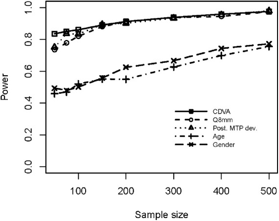
Power analysis results for CDVA, Q_8mm, posterior minimum thickness point deviation, age, and gender.

Graphics User Interface

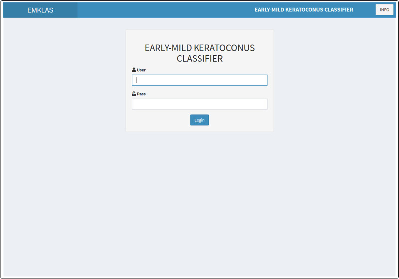
A web application containing the pre-trained model was created to allow users to instantly estimate the probability of an individual belonging to each modeled group using a minimal set of parameters. This application (Fig. 6) was developed with Shiny v1.3.2 (RStudio, Inc.),²⁴ and it was deployed within the institutional intranet using the ShinyAuthr v0.0.99 authentication module (Paul Campbell) to prevent access by unauthorized users.²⁵

Figure 6.

Application landing page showing the log-in form with a secured authentication layer.

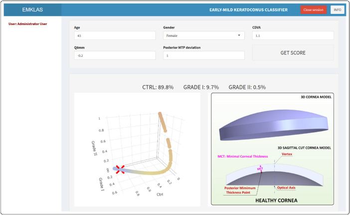
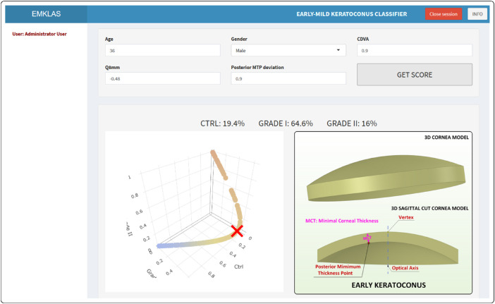
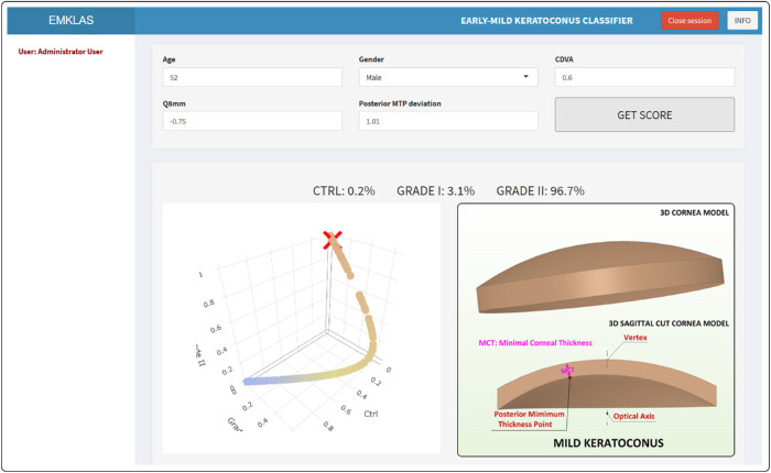
The landing page for the application (Fig. 6) originally was a log-in form that added a secured authentication layer. Over time, as registration capabilities were disabled, new users were added by the system administrator. After log-in, the application exhibits a form composed of five text boxes that correspond to the model predictors, each filled in by default with typical values for a healthy individual. After inserting any new desired values and pressing the “GET SCORE” button, the trained model makes its prediction (Figs. 7⁸–9) by providing an early or mild KC classification score (EMKLAS) as a percentage and by depicting a typical cornea, including some of the main parameters considered in the prediction.

Figure 7.

Screenshot of a healthy individual (control) with the typical 3D virtual corneal model schematic representation.

Figure 8.

Screenshot of an early KC individual (RETICS) with the typical 3D virtual corneal model schematic representation.

Figure 9.

Screenshot of a mild KC individual (RETICS) with the typical 3D virtual corneal model schematic representation.

Figures 7 to 9 are screen captures of one healthy individual (43-year-old female, oculus dexter [OD], CDVA = 1, Q_8mm = –0.2, posterior minimum thickness point deviation = 0.1), one patient with early KC (36-year-old male, OD, CDVA = 0.9, Q_8mm = –0.48, posterior minimum thickness point deviation = 0.9), and one patient with mild KC (52-year-old male, OD, CDVA = 0.6, Q_8mm = –0.75, posterior minimum thickness point deviation = 0.94), respectively. Each one also includes a 3D image of a typical cornea that represents how different predictors were calculated based on physical measurements.

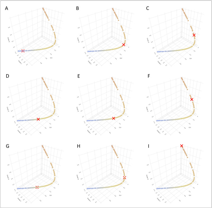
Some cases, however, were incorrectly classified by our graphical user interface (GUI) due to the singularities characterizing KC. Figure 10 includes some screenshots from different individuals representing all of the possible model classes. Patients A, B, and C were healthy individuals; patients D, E, and F had early KC; and patients G, H, and I had mild KC. Patient A, a 43-year-old female, was correctly classified as healthy and appears on the lower left end of the score line. Patient B, a 54-year-old male, was incorrectly classified as early KC. Patient C, a 47-year-old male, was incorrectly classified as mild KC. Patient D, a 30-year-old male, was incorrectly classified as healthy. Patient E, a 36-year-old male, was correctly classified as early KC. Patient F, a 28-year-old male, was incorrectly classified as mild KC. Patient G, a 79-year-old male, was incorrectly classified as healthy. Patient H, a 57-year-old male, was incorrectly classified as early KC. Finally, patient I, a 52-year-old male, was correctly classified as mild KC.

Figure 10.

Screenshots representing all of the possible classes in the model. The top row corresponds to true healthy individuals, predicted as healthy (A), early KC (B), or mild KC (C). The middle row corresponds to the true early KC individuals predicted as healthy (D), early KC (E), or mild KC (F). Finally, the bottom row refers to the true mild KC individuals predicted as healthy (G), early KC (H), or mild KC (I).

In essence, the GUI application is an approachable design accessible from any network-connected terminal, no matter what computer, tablet, or smartphone is used. It works with most of the widely used operating systems, and it does not require installing any drivers or software, as long as the web browser is up to date. It also automatically adjusts the screen layout to fit different screen sizes and orientations, thus making it more accessible and user friendly.

Discussion

Given the multifactorial nature of KC, early KC detection is usually approached by making an optimal evaluation of risk factors.² However, the detection of KC in its primary preclinical forms remains a clinical challenge, as most research has presented models based on a wide variety of parameters that strongly depend on the characteristics of the analyzed sample.⁴ Several robust predictive models for detecting incipient KC manifestations have been published in the scientific literature, although the lack of standardization makes their comparison difficult.

One of the main problems that ophthalmologists currently encounter is that experts have not reached an agreement about how early corneal ectasia should be characterized.^5–11 This is due to the ambiguity surrounding the disease definition in its preclinical phase,^4,8 the size of the samples used for these studies,⁴ and the fact that most of the indices employed for disease detection are technology specific, thus rendering them non-interchangeable.^4,28 Hallak and Azar²⁹ suggested a possible solution to this problem through the use of artificial intelligence (AI): “AI will help with screening patients, improving diagnoses, and suggesting personalized treatments.”

In this study, therefore, we have defined a predictive model based on a set of optimal demographic, optical, and geometric factors measured by only one technology. This approach allows us not only to assess the current degree of disease development based on the level of a patient's visual limitation but also to define the probability of correctly classifying each case. As far as the authors know, no previous studies have successfully combined demographic, optical, pachymetric, and morphogeometric variables in a real-time environment to detect and classify healthy, early KC, and mild KC eyes.

Expressing the probability of correctly classifying a patient as a score offers several benefits. First, reducing information from varied parameters of a diverse nature into a single and simple to understand parameter minimizes the risk of overlooking important information. In fact, this risk can be quite high, as typical analytical reports frequently include long lists of various parameters over several pages that must be read fairly quickly, and they rarely include associated normality intervals.

This approach also allows assessment of the joint actions of diverse parameters. Detecting the existence of a disease when a key parameter shows a significantly high or low value can be simple, but detection becomes more difficult when minor variations of several key parameters are present. In this case, the use of a score may help ophthalmological professionals make their assessments because it offers an objective and quantitative scale that addresses all possible parameter relations.

Table 7 shows that the results of several studies in which models were obtained by Scheimpflug technologies fall in line with ours.^6,8,30 Hwang et al.⁸ proposed a detection model that combined five parameters (index height decentration, index vertical asymmetry, pachymetry apex, inferior-superior value, and Ambrosio's relational thickness maximum variability), with area under the curve (AUC) = 0.86, sensitivity of 83%, and specificity of 83%. Similar results have been obtained by other researchers^6,30 at the model development stage, depending on the limited metrics of Scheimpflug technology.

Table 7.

Comparison of the Current Study with Earlier Studies

	Sample Size (Eyes)
Study	KC Group	Control Group	Technology Used and Degree of KC Detected/Classified	Total Parameters Considered/Best Parameters Used	Area Under Curve	Sensitivity (%)	Specificity (%)
Current study	74	104	Sirius Scheimpflug tomography + geometric modeling Detects early and mild KC Classifies according to RETICS scale (grade I to grade IV+)	Combination of 27 demographic, clinical, pachymetric, and geometric parameters Age, gender, CDVA, Q8mm, and posterior MCT point deviation	Healthy, 0.87 (training) Early KC, 0.69 (training) Mild KC, 0.94 (training)	Healthy, 84 Early KC, 57 Mild KC, 63	Healthy, 73 Early KC, 82 Mild KC, 97
Hwang et al. (2018)8	30	60 (Post-LASIK)	Pentacam Scheimpflug tomography and SD-OCT imaging Detects asymmetric KC eyes (preclinical) No classification	Combines 9 tomography with 15 OCT variables 5 Scheimpflug variables 13 variables from both Scheimpflug and SD-OCT devices	Not mentioned	83; 100	83; 100
Shajari et al. (2018)30	27 (unilateral KC in fellow eye)	50	Pentacam Scheimpflug tomography Detects asymptomatic early KC No classification	18 variables from Scheimpflug device Index of height decentration and index of vertical asymmetry	0.79 (IHD); 0.72 (IHA)	Not mentioned	Not mentioned
Saad et al. (2010)10; Saad et al. (2012)31	40 FFKC + 31 KC	72	Orbscan IIz and OPD-Scan Detects FFKC (early) and KC (mild) No classification	54 variables and 6 discriminant functions	N vs. FFKC, 0.98 N vs. KC, 0.99	N vs. FFKC, 93 N vs. KC, 97	N vs. FFKC, 0.92 N vs. KC, 100
Qin et al. (2013)32	84	67	RTVue Fourier-domain OCT Detects clinical KC No classification	5 pachymetric variables Logistic regression formula	0.98	90.5	95.0

Table 7.

Continued

	Sample Size (Eyes)
Study	KC Group	Control Group	Technology Used and Degree of KC Detected/Classified	Total Parameters Considered/Best Parameters Used	Area Under Curve	Sensitivity (%)	Specificity (%)
Rabinowitz et al. (2014)33	46 moderate 54 early 7 FFKC 16 suspect	180	TMS-4 videokeratographer, RTVue Fourier-domain OCT, and Hartmann–Shack aberrometer Detects and classifies normal, FFKC, and suspect, early, and moderate KC	A combination of videokeratography and OCT indices (I-S value and minimum pachymetry) and PA/I-S	Not mentioned	Moderate, 100 Early, 100 FFKC, 100 Suspect, 63	Moderate, 100 Early, 100 FFKC, 97 Suspect, 98
Silverman et al. (2017)34	30	111	Pentacam Scheimpflug tomography and Artemis very-high-frequency ultrasound Detects clinical KC	105 Artemis and 96 Pentacam variables Combination of 3 Artemis and 4 Pentacam parameters	>0.99	97	100
Yousefi et al. (2018)35	796 FFKC 390 KC	1970	Casia OCT Detects FFKC (early) and KC (mild) Four clusters according to the Casia ESI and diagnostic labeling convention	420 parameters 2 eigen parameters	Not mentioned	N vs. KC, 97	N vs. KC, 96

CDVA, corrected distance visual acuity; ESI, ectasia status index; FFKC, forme fruste keratoconus; I-S, inferior–superior keratometric difference; KC, keratoconus; MCT, minimum corneal thickness; N, normal; OCT, optical coherence tomography; PA/I-S, pachymetry/asymmetry index; RETICS, Thematic Network for Co-Operative Research in Health; SD-OCT, spectral-domain optical coherence tomography.

Other researchers have relied on multivariate systems to combine the use of two different technologies. Saad and Gatinel¹⁰ created a model with 54 variables and six discriminant functions with 93% sensitivity and 92% specificity. It was validated in a posterior study,³¹ with sensitivity and specificity values of 92% and 96%, respectively. These values are slightly better than those we obtained when discerning control (91% sensitivity, 80% specificity) and mild KC (97% sensitivity, 89% specificity) and are considerably better than our results for the early KC group (64% sensitivity, 80% specificity). However, this model used two different technologies, whereas ours employs only one.

Other research has proposed combining a set of different technologies.^32–34 In these cases, however, the authors established a KC suspect profile for suffering KC in a later stage, as they included subjects with manifest inferior steepening.⁴

The latest KC severity classification tendencies indicate the use of machine learning-based approaches. Yousefi et al.³⁵ utilized an unsupervised machine learning analysis of over 420 parameters to classify 3156 eyes with only two eigen parameters. They reported 97.7% sensitivity and 94.1% specificity. However, these values were obtained in comparison with the CASIA ectasia screening index (ESI), so they cannot be generalized to the parameters generated by other technologies such as Sirius or Pentacam. Moreover, clinical diagnosis labels were not available in their study; hence, its accuracy could not be assessed. The same authors recently took this study even further and proposed a machine-learning model that predicts the likelihood of needing keratoplasty interventions.³⁶ Lavric and Valentin³⁷ implemented an algorithm that uses convolutional neural networks to detect the presence of KC with an accuracy of 99.33%, but this method uses topographic pictures of merely the anterior cornea surface and, as the device employed was Pentacam, the results were valid only for this technology.

Our classifier uses an ordinal logistic regression model that combines 27 parameters, obtaining an overall accuracy of 73% (95% CI, 65–79) in the training phase. This means that the model has correctly classified more than 70% of cases and has proven to be particularly accurate for the control and mild KC groups, with accuracies of 83% to 84%, respectively. The early KC group presented the lowest accuracy (70%), with 26 cases of 61 incorrect classifications. This can be explained by the difficulty of detecting KC in its early development stages, due to the consistency in corneal thickness that the corneal structure presents even when changing from a healthy scenario to a mild KC one, as the nine examples shown in Figure 10 demonstrate.

This early and mild KC classifier has been trained by taking the diagnostics made by ophthalmological professionals as the gold standard, which unavoidably implies some undetermined amount of subjective information was used. During the fitting procedure, the model attempted to find a generalization linking predictors with prediction while maximizing performance. Nonetheless, some cases may involve certain samples not matching any kind of generalization given the subjective nature of the training data, making it difficult to establish a clear well-defined boundary between groups.

Uncertainty has always been considered a given in medical practice.³⁸ Eyes without a clear EMKLAS value for any of the groups (below 95%) could present some clinical peculiarities that make them different. Alternatively, they may correspond to evolutive cases in which some parameters change more quickly than others. A prospective study of these cases would be necessary to set an accurate decision threshold for considering a case to be KC suspect. In any case, when considering that wrongly classifying KC degrees is less important than classifying a diseased patient (early or mild) as healthy, the probabilities of belonging to both KC groups I and II can be summed in those uncertain cases to achieve the best diagnostic accuracy. In line with the doctor's criterion, any case of suspected KC should receive further clinical consultation.

Consequently, the presence of a certain lack of accuracy is something we can expect and does not necessarily mean that the model fitting ability fails. Our model has quantitatively confirmed the difficulty of distinguishing between groups, as the degree of misclassification between adjacent groups (control vs. early KC; early KC vs. mild KC) reached 26.4% of incorrectly classified patients when false-positives and false-negatives were combined, thus confirming the utility of our tool.

In this research, the AUC, specificity, and sensitivity of the model attained after the inner validation process suggest high performance, with AUC values of 0.87, 0.69, and 0.94 for the control, early KC, and mild KC groups, respectively. These specificity and sensitivity figures are slightly better that those obtained in the training stage in all cases, except for specificity for the control group, which was slightly lower (see Table 5).

The independent validation of the ordinal logistic regression model showed an overall accuracy of 71% (95% CI, 55–84), suggesting that, even though the obtained quality figures were slightly lower (with accuracies of 79%, 69%, and 80% for the control, early KC, and mild KC groups, respectively), the results generally fall in line with those obtained in the internal bootstrap validation procedure, as Table 6 shows. This indicates that the validated performance of the model is fairly good, even though the decisions based on the ordinal logistic regression model should be made cautiously, and it would be advisable to repeat the training process of the model with a bigger independent sample to validate the results.

Our study also presents some limitations. Apart from the previously mentioned subjectivity induced by using diagnostics made by ophthalmological professionals as the gold standard for model training, the sample size was limited by our inclusion criteria because we preferred to ensure that evaluated eyes were truly subclinical KC ones. It should also be taken into account that clinical metrics strongly depend on the technology used for their measure,²⁸ so our results can be considered valid only for those eyes tested using Sirius tomography.

In conclusion, in this work we have developed a GUI based on an ordinal logistic regression model that assesses the current degree of KC development and defines the probability of correctly classifying each case. Our model correctly classified more than 70% of cases and was particularly accurate for the control (79%) and mild KC (80%) groups, whereas the accuracy for the early KC group was considerably lower (69%). Thus, repeating the training process with a bigger sample using different data should be considered to improve these results. Although ordinal logistic regression is a widely used, state-of-the-art tool for biomedical data research, other techniques, such as deep learning, can be used to improve the quality of the results obtained.

References

- 1. Ferdi AC, Nguyen V, Gore DM, Allan BD, Rozema JJ, Watson SL. Keratoconus natural progression: a systematic review and meta-analysis of 11,529 Eyes. Ophthalmology. 2019; 126: 935–945. [DOI] [PubMed] [Google Scholar]
- 2. Martinez-Abad A, Pinero DP. New perspectives on the detection and progression of keratoconus. J Cataract Refract Surg. 2017; 43: 1213–1227. [DOI] [PubMed] [Google Scholar]
- 3. Randleman JB, Russell B, Ward MA, Thompson KP, Stulting RD. Risk factors and prognosis for corneal ectasia after LASIK. Ophthalmology. 2003; 110: 267–275. [DOI] [PubMed] [Google Scholar]
- 4. Lin SR, Ladas JG, Bahadur GG, Al-Hashimi S, Pineda R. A review of machine learning techniques for keratoconus detection and refractive surgery screening. Semin Ophthalmol. 2019; 34: 317–326. [DOI] [PubMed] [Google Scholar]
- 5. Binder PS. Risk factors for ectasia after LASIK. J Cataract Refract Surg. 2008; 34: 2010–2011. [DOI] [PubMed] [Google Scholar]
- 6. Binder PS, Trattler WB. Evaluation of a risk factor scoring system for corneal ectasia after LASIK in eyes with normal topography. J Refract Surg. 2010; 26: 241–250. [DOI] [PubMed] [Google Scholar]
- 7. Chan C, Ang M, Saad A, et al.. Validation of an objective scoring system for forme fruste keratoconus detection and post-LASIK ectasia risk assessment in Asian eyes. Cornea. 2015; 34: 996–1004. [DOI] [PubMed] [Google Scholar]
- 8. Hwang ES, Perez-Straziota CE, Kim SW, Santhiago MR, Randleman JB. Distinguishing highly asymmetric keratoconus eyes using combined Scheimpflug and spectral-domain OCT analysis. Ophthalmology. 2018; 125: 1862–1871. [DOI] [PMC free article] [PubMed] [Google Scholar]
- 9. Randleman JB, Woodward M, Lynn MJ, Stulting RD. Risk assessment for ectasia after corneal refractive surgery. Ophthalmology. 2008; 115: 37–50. [DOI] [PubMed] [Google Scholar]
- 10. Saad A, Gatinel D. Topographic and tomographic properties of forme fruste keratoconus corneas. Invest Ophthalmol Vis Sci. 2010; 51: 5546–5555. [DOI] [PubMed] [Google Scholar]
- 11. Seiler T, Quurke AW. Iatrogenic keratectasia after LASIK in a case of forme fruste keratoconus. J Cataract Refract Surg. 1998; 24: 1007–1009. [DOI] [PubMed] [Google Scholar]
- 12. Nesburn AB, Bahri S, Salz J, et al.. Keratoconus detected by videokeratography in candidates for photorefractive keratectomy. J Refract Surg. 1995; 11: 194–201. [PubMed] [Google Scholar]
- 13. Choi RY, Coyner AS, Kalpathy-Cramer J, Chiang MF, Campbell JP. Introduction to machine learning, neural networks, and deep learning. Transl Vis Sci Technol. 2020; 9: 14. [DOI] [PMC free article] [PubMed] [Google Scholar]
- 14. Cavas-Martínez F, Fernández-Pacheco DG, Parras D, Cañavate FJF, Bataille L, Alió J. Study and characterization of morphogeometric parameters to assist diagnosis of keratoconus. Biomed Eng Online. 2018; 17: 161. [DOI] [PMC free article] [PubMed] [Google Scholar]
- 15. Cavas-Martínez F, Bataille L, Fernández-Pacheco DG, Cañavate FJF, Alio JL. Keratoconus detection based on a new corneal volumetric analysis. Sci Rep. 2017; 7: 15837. [DOI] [PMC free article] [PubMed] [Google Scholar]
- 16. Romero-Jimenez M, Santodomingo-Rubido J, Wolffsohn JS. Keratoconus: a review. Cont Lens Anterior Eye. 2010; 33: 157–166; quiz 205. [DOI] [PubMed] [Google Scholar]
- 17. Alio JL, Pinero DP, Aleson A, et al.. Keratoconus-integrated characterization considering anterior corneal aberrations, internal astigmatism, and corneal biomechanics. J Cataract Refract Surg. 2011; 37: 552–568. [DOI] [PubMed] [Google Scholar]
- 18. Vega-Estrada A, Alio JL, Brenner LF, et al.. Outcome analysis of intracorneal ring segments for the treatment of keratoconus based on visual, refractive, and aberrometric impairment. Am J Ophthalmol. 2013; 155: 575–584. [DOI] [PubMed] [Google Scholar]
- 19. Huseynli S, Salgado-Borges J, Alio JL. Comparative evaluation of Scheimpflug tomography parameters between thin non-keratoconic, subclinical keratoconic, and mild keratoconic corneas. Eur J Ophthalmol. 2018; 28: 521–534. [DOI] [PubMed] [Google Scholar]
- 20. Agresti A. Categorical Data Analysis. 3rd ed New York: Wiley-Interscience; 2012. [Google Scholar]
- 21. Venables WN, Ripley BD. Modern Applied Statistics with S. New York: Springer-Verlag; 2002. [Google Scholar]
- 22. Efron B, Tibshirani R. Improvements on cross-validation: the 632+ bootstrap method. J Am Stat Assoc. 1997; 92: 548–560. [Google Scholar]
- 23. R Core Team. The R Project for statistical computing. Available at: https://www.R-project.org/. Accessed May 13, 2020.
- 24. Chang W, Cheng J, Allaire J, Xie Y, Jonathan M. Shiny: web application framework for R. Available at: https://CRAN.R-project.org/package=shiny. Accessed May 13, 2020.
- 25. Campbell P. PaulC91/shinyauthr: Shiny authentication modules. Available at: https://rdrr.io/github/PaulC91/shinyauthr/. Accessed May 13, 2020.
- 26. Aberson CL. Applied Power Analysis for the Behavioral Sciences. 2nd ed Boca Raton, FL: Taylor & Francis; 2019. [Google Scholar]
- 27. Demidenko E. Sample size determination for logistic regression revisited. Stat Med. 2007; 26: 3385–3397. [DOI] [PubMed] [Google Scholar]
- 28. Savini G, Carbonelli M, Sbreglia A, Barboni P, Deluigi G, Hoffer KJ. Comparison of anterior segment measurements by 3 Scheimpflug tomographers and 1 Placido corneal topographer. J Cataract Refract Surg. 2011; 37: 1679–1685. [DOI] [PubMed] [Google Scholar]
- 29. Hallak JA, Azar DT. The AI revolution and how to prepare for it. Transl Vis Sci Technol. 2020; 9: 16. [DOI] [PMC free article] [PubMed] [Google Scholar]
- 30. Shajari M, Jaffary I, Herrmann K, et al.. Early tomographic changes in the eyes of patients with keratoconus. J Refract Surg. 2018; 34: 254–259. [DOI] [PubMed] [Google Scholar]
- 31. Saad A, Gatinel D. Validation of a new scoring system for the detection of early forme of keratoconus. Int J Kerat Ect Cor Dis. 2012; 1: 100–108. [Google Scholar]
- 32. Qin B, Chen S, Brass R, et al.. Keratoconus diagnosis with optical coherence tomography-based pachymetric scoring system. J Cataract Refract Surg. 2013; 39: 1864–1871. [DOI] [PMC free article] [PubMed] [Google Scholar]
- 33. Rabinowitz YS, Li X, Canedo ALC, Ambrósio R Jr Bykhovskaya Y. Optical coherence tomography combined with videokeratography to differentiate mild keratoconus subtypes. J Refract Surg. 2014; 30: 80–87. [DOI] [PMC free article] [PubMed] [Google Scholar]
- 34. Silverman RH, Urs R, RoyChoudhury A, Archer TJ, Gobbe M, Reinstein DZ. Combined tomography and epithelial thickness mapping for diagnosis of keratoconus. Eur J Ophthalmol. 2017; 27: 129–134. [DOI] [PMC free article] [PubMed] [Google Scholar]
- 35. Yousefi S, Yousefi E, Takahashi H, et al.. Keratoconus severity identification using unsupervised machine learning. PLoS One. 2018; 13: e0205998. [DOI] [PMC free article] [PubMed] [Google Scholar]
- 36. Yousefi S, Takahashi H, Hayashi T, et al.. Predicting the likelihood of need for future keratoplasty intervention using artificial intelligence. Ocul Surf. 2020; 18: 320–325. [DOI] [PubMed] [Google Scholar]
- 37. Lavric A, Valentin PJ. Ci, neuroscience. KeratoDetect: keratoconus detection algorithm using convolutional neural networks. Comput Intell Neurosci. 2019; 2019: 8162567. [DOI] [PMC free article] [PubMed] [Google Scholar]
- 38. Kim K, Lee Y-M. Understanding uncertainty in medicine: concepts and implications in medical education. Korean J Med Educ. 2018; 30: 181–188. [DOI] [PMC free article] [PubMed] [Google Scholar]