Monte Carlo Simulation of Brownian Motion using a Piezo-Actuated Microscope Stage

Abstract

Single particle tracking is a powerful tool for studying and understanding the motions of biological macromolecules integral to cellular processes. In the past three decades there has been continuous and rapid development of these techniques in both optical microscope design and in algorithms to estimate the statistics and positions of the molecule’s trajectory. Although there has been great progress, comparison between different microscope configurations and estimation algorithms has been difficult beyond simulated data. In this paper we explore using a piezo actuated microscope stage to reproduce Brownian motion. Our goal is to use this as a tool to test performance of single particle tracking optical microscopes and estimation algorithms. In this study, Monte Carlo simulations were used to assess the ability of piezo actuated microscope stages for reproducing Brownian motion. Surprisingly, the dynamics of the stage together with configuration of the system allow for preservation of the Brownian motion statistics. Further, feed forward model inverse control allows for low error tracking of Brownian motion trajectories over a wide range of diffusion constants, varying stage response times, and trajectory discrete time steps. These results show great promise in using a piezo actuated microscope stage for testing single particle tracking experimental setups.

I. Introduction

The study of biology has utilized microscopes for over a century to understand life at the smallest scales. Through both evolving instrumentation and algorithm development, the resolving power of these microscopes continues to increase, allowing for cellular processes to become the focus of much research. Underlying these process are small molecules, proteins, RNA, and other bio-molecules that transduce signals, and shape the response of the cell in its environment. Studying the motions of these molecules allow us to understand typical cell function and malfunction, which are important in understanding cellular origins of disease, understanding mechanisms of viral infection, and other applications. Among the techniques, algorithms, and instrumentation to study nature at this level is a class termed single particle tracking (SPT). SPT optical microscopes combine photodetectors, light sources, optics, actuators, stages, and the sample being studied. Control systems, signal processing and estimation techniques all come together to enable SPT to break through the optical diffraction limits, allowing the study of these processes at much smaller lengths scales, and with much higher temporal resolution than before. It is now possible to localize and track single particles with uncertainties on the order of 1 to 100 nm over long time periods. Although comprehensive reviews and comparisons between techniques have been done in the past [1], [2], they have relied on physically realistic simulations. One of the main benefits of a simulation-based approach is the existence of a known ground truth. However, while such simulations can be very accurate and account for a great deal of the experimental realities, they are almost by definition unable to capture all the specifics of any one experimental setup. Alternatively, one can perform careful, controlled experiments on real systems but then typically the knowledge of ground truth is not possible, making comparisons beyond simulated data very difficult to do. We would like to start bridging this gap by developing techniques to assess performance of both SPT optical microscopes and related estimation algorithms. This paper describes the control of a piezo-actuated microscope stage to reproduce Brownian motion trajectories. We envision that this may be used to assess both SPT optical microscopes as well as localization algorithms.

SPT has developed alongside related techniques termed super-resolution over the last thirty years in order to study cell structure and processes at the nanometer scale [3]. These setups are based on standard or home-built microscope which focus light onto the sample [4]. Fluorescent indicators are added to the cells with targeting sequences enabling the specific labeling of proteins, molecules, organelles and other structures within the cell [5], [6]. These indicators absorb the incident excitation light and emit incoherent light at longer wavelengths. An optical filter then separates the excitation light from the emitted light allowing for an image to be formed from only the labeled structures in the cell. One can often view this image by eye through the microscopes eyepiece, or by recording the image using a scientific camera and saving the resulting images for later analysis. There are two general forms of this fluorescence microscope used in SPT. The first, a widefield microscope, is one that employs a scientific camera with typically 1–10 megapixels to capture an entire field of view simultaneously. The second, a confocal microscope, uses a single element optical detector that is coaligned to laser illumination. For confocal SPT, the position of the laser in the sample is controlled by a suitable control law based on signal feedback from the photodetector [7], [8].

The application of SPT using either widefield or confocal microscopy is an indispensable tool in the study of biomolecular transport. However, comparisons of SPT performance are difficult on physical hardware. Both hardware performance and algorithms may potentially be assessed using standard piezo-actuated microscope stages to reproduce the motions of single particles. Under this scheme, fluorescent particles are fixed on a microscope slide and moved along a known Brownian motion trajectory by the piezo stage while the microscope is observing and recording their motion. After the localization and estimation is completed on the recorded data, it can be compared to the known ground truth of the Brownian motion trajectory. This would enable a new way to assess the performance of these systems. The first step to realizing this is to understand the limits to which a microscope stage can reproduce molecular motions.

The remainder of this paper is organized as follows. In the next section, we briefly review Brownian motion and methods for analyzing the statistics of time series data generated by such models. In Sec. III, we describe and compare two different feedback structures which can generate Brownian trajectories to reproduce the motion of single particles under the observation of a microscope. Monte-Carlo simulations were used to understand the systems characteristics and analyze their performance. Next, in Sec. IV, we assess the limitations of the better performing system in simulating the range of Brownian motion for both confocal and widefield microscopes and apply feedforward model inverse control to improve the performance of Brownian motion reproduction using a microscope stage. Finally, we provide a few concluding remarks in Sec. V.

II. Brownian Motion

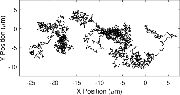
Brownian motion was first observed by an ancient philosopher watching dust particles dance about in air illuminated by rays of sunlight. However, the topic was not studied to any depth until after Robert Brown’s publication of his observations of the motions of pollen grains suspended in water [9]. An example of this motion is shown in Fig. 1. In 1905, Einstein described Brownian motion as a free unconstrained motion subject to a randomly fluctuating force. The theories of Brownian motion were further developed as the fields of applied probability, stochastic differential equations, and stochastic signals and systems were developed. Many texts now describe Brownian motion alongside treatments on related topics such as random walks and Gaussian distributed white noise, laying the groundwork for understanding these processes [9], [10].

Fig. 1.

An example of Brownian motion

A particular description of Brownian motion in discrete time is given by

$$Y_n=Y_{n-1}+U_n,U_n\sim \mathcal{N}(0,2D\mathrm{\Delta }T),$$ (1)

were Y_n and Y_n−1 represents the particle position at time point n and n−1 respectively and U_n is a zero-mean Gaussian random variable with a variance defined by the product of the diffusion constant D, the discrete time step ΔT. As time progresses, the variance of the distribution of possible positions at time point n given its initial location increases, describing a tendency for a particle moving according to (1) to spread out as time increases. The diffusion constant, often measured in units of $\frac{\mu {\text{m}}^2}{\text{s}}$ in SPT, describes the rate of change of the variance of the PDF, characterizing the speed at which the distribution of the possible positions of the particle spreads out in space. In the context of cellular biology, typical diffusion constants are in the range of $0.001-50\frac{\mu {\text{m}}^2}{\text{s}}$.

Although the statistics of the generated trajectories of the ensemble motions are very useful in understanding subcellular phenomena, each particle traces a particular trajectory in space and time. This sample path of an individual particle is also extremely informative. The power spectrum, S, of this motion is given by

$$S(\omega )=\frac{S_0}{{\omega }^2},$$ (2)

and is characterized by a decrease of 20 dB/decade of frequency ω [10]. This indicates that more information about the shape of the trajectory is encoded at lower frequencies compared to higher frequencies. This may allow for low pass filtering to occur with minimal impact on the overall trajectory, smoothing out the small scale motion while keeping the large scale shape of the trajectory intact. As the bandwidth of a low pass filter is decreased, the trajectory increasingly deviates from the ideal Brownian motion trajectory potentially changing the underlying parameters of the Brownian motion, in particular the diffusion constant. Since the physical mechanics of a piezo stage act in essence as a low pass filter, it is important to characterize the ability of the mechanical system to preserve the underlying parameter values when simulating Brownian motion.

The simulation accuracy and performance of Brownian motion can be characterized in a few different ways. These methods can be collected into broader catagories such as: statistical distance of single time step probability distribution (SSPDF), mean squared displacement (MSD), trajectory similarity, frequency domain analysis, and analysis of tracking error over time. In our study we used the Kullback-Leilbler divergence (KL) to assess statistical distance between SSPDFs as well as the MSD and stage tracking error to understand how well a piezo-actuated stage can reproduce Brownian motion. (It should be noted that in the biophysical community, perhaps the most common approach to analyze SPT trajectories is to use the MSD.) An ideal Brownian motion will have a Gaussian distributed SSPDF with a variance that is a function of the diffusion constant D (specifically, a variance kDΔT). A motion that does not exhibit this behavior indicates a departure from ideal Brownian motion and will result in a KL divergence larger than 0. Since the KL divergence is not a true distance measure, it gives a different value depending on the order of distributions used. We used the discrete formulation of KL divergence

$$KL\left(f_{Stage}\mid f_{Traj}\right)=\sum f_{Stage}\ln \left(\frac{f_{Stage}}{f_{Traj}}\right),$$ (3)

where f_stage and f_Traj represents the SSPDF of the stage motion and the trajectory respectively. The MSD assesses the variance of the particle’s displacement as a function of time [11]. For an ideal Brownian motion, the MSD is a linear function with a slope related to the diffusion constant of the single particle and an intercept of zero,

$$MSD[n]=\langle {\left(Y_n-Y_0\right)}^2\rangle =2D\mathrm{\Delta }Tn.$$ (4)

Any deviation from the functional relationship indicates departure from idea Brownian motion. Note that in this work we are ignoring the measurement noise on the trajectories when calculating the MSD since we are working with ground truth. Such noise can be included by shifting the intercept of the MSD by $2{\sigma }_N^2$ where ${\sigma }_N^2$ is the variance of the measurement noise, typically assumed to be zero mean and Gaussian.

III. Simulation of Brownian Motion Filtered by Dynamical System

A. System Description

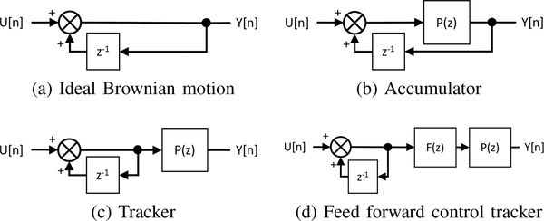
As illustrated in Fig. 2, simulating Brownian motion with a physical setup can take many forms depending on the placement of the piezo stage within the system. We focus on two physically realizable configurations that we call the accumulator and the tracker. In both configurations, the input U(z) is a sample path from a zero-mean Gaussian white noise process with a variance proportional to the diffusion constant of the Brownian motion. Feedback of the output is shifted by one time step and then summed with the input. The key difference of these two systems is where the filtering from the piezo-actuated microscope stage occurs relative to the branch point of the feedback with the stage placed before the branching point for the accumulator and after for the tracker. This difference has a large impact on the resulting errors of the systems, especially when the system time constant is larger than the discrete time step. We note that it is of course possible to introduce more complexity in the system to achieve a better physical simulation. However, keeping the overall system as simple as possible may be advantageous in getting researchers in the biophysical community to adopt these methods. We note also that in general the transfer function P(z) represents the physical piezo-stage as well as any closed-loop controllers.

Fig. 2.

Discrete time block diagrams for modeled systems

B. Simulation

Monte-Carlo simulations were employed in two distinct phases in order to understand these two systems and their performance in terms of capturing an ideal Brownian motion. The first phase compared the two systems using the MSD and the tracking error. As discussed in Sec. III.C below, this phase indicated that the tracker was the better-performing structure. The second phase then focused on the tracker, analyzing its performance to different kinds of parameters. All simulations used 10,000 sets of inputs of 5000 samples each. In the first phase, the inputs represent Gaussian white noise, and were generated by creating an array of normally distributed random numbers multiplied by the motion model variance (1). In the second stage, the array of normally distributed random numbers were cumulatively summed to create Brownian motion sample paths. These paths were then input directly to P(z). In these simulations, the piezo-actuated microscope stage was modeled as a first order system. This representation was chosen because many controllers/amplifiers of the piezo-actuated stages incorporate proportional-integral control to mitigate drift and hysteresis of the piezo actuators and achieve good tracking of the reference input. As a result, the closed-loop system is close to first order at lower frequencies. The continous dynamics of the stage were modeled using an exact discretization given by

$$P[z]=\frac{1-e^{-\frac{\mathrm{\Delta }T}{\tau }}}{z-e^{-\frac{\mathrm{\Delta }T}{\tau }}}.$$ (5)

It is important to highlight that using the exact discretization means that the piezo system is essentially moving continuously in the simulations, not at the simulation time step.

Using the stage transfer function together with each system configuration results in difference equations for the Accumulator given by

$$Y_n=e^{-\frac{\mathrm{\Delta }T}{\tau }}{Y}_{n-1}+(1-e^{-\frac{\mathrm{\Delta }T}{\tau }})Y_{n-2}+(1-e^{-\frac{\mathrm{\Delta }T}{\tau }})U_{n-2}.$$ (6)

and for the Tracker given by

$$Y_n=(1+e^{-\frac{\mathrm{\Delta }T}{\tau }})Y_{n-1}-e^{-\frac{\mathrm{\Delta }T}{\tau }}{Y}_{n-2}+(1-e^{-\frac{\mathrm{\Delta }T}{\tau }})U_{n-1}.$$ (7)

C. System Comparison

Using a Monte Carlo approach, we compared how well the two systems can match the Brownian motion trajectory over time by analyzing their MSD and error. A discrete time step of ΔT = 100 ms, a system time constant of τ =100 ms, and a diffusion constant of D =1 μm²/s were used (first line in Table I).

TABLE I.

Simulation Parameters

Simulation	D (μm2/s)	ΔT (ms)	τ (ms)
System Comparison	1	100	100
$\frac{\mathrm{\Delta }T}{\tau }$ sweep	1	1–1000	1–1000
Diffusion Rate sweep	10−6 – 106	1–1000	1–1000
Feed Forward Control	1	1	12.5

The results are shown in Fig. 3. We can see that both systems initially exhibit MSD curves that are substantially different from Brownian motion. However, the tracker MSD slope converges to that of Brownian motion. In contrast, the accumulator asymptotically converges to a value that is different for both the MSD and the MSD slope. As a result, the tracker will reproduce Brownian motion with the desired diffusion constant, while the accumulator will give Brownian motion with a diffusion constant that is different than the desired value. In addition, while the accumulator and tracker have error variances that start out approximatly the same, the error on the accumulator grows without bound while the tracker quickly reaches an asymptotic value. While it is possible that modifications to the accumulator system may mitigate these issues, further complexity may hinder adoption in the SPT community.

Fig. 3.

Comparison between Accumulator (dashed) and Tracker (dotted) models. (a) Comparison of MSD against a true Brownian motion sample path trajectory. (b) Slope in the MSD curve and (c) variance in tracking error of the system output and the Brownian motion sample path.

The difference in the performance between these two systems centers on the location of the branching point relative to the plant. The system input can be regarded as a series of step inputs and the response of the stage, is described by a first order system at a time equal to the discrete time step ΔT, giving a basic exponential response for the error ϵ, where the effective time constant is the ratio of the simulation step and the system time constant,

$$ϵ=e^{-\frac{\mathrm{\Delta }T}{\tau }}.$$ (8)

For the accumulator, the output of the stage is then fed back and summed with the next input. This allows the error to compound every time step making the error grow without bound as the system tries to “catch up” to the Brownian motion trajectory. The resulting output fails to capture the statistics of the input, leading to a different effective diffusion coefficient.

By contrast, the tracker converges quickly to the desired value of the diffusion constant and the error reaches a steady state value. This can again be understood through looking at U[n] as a sequence of step inputs. The system essentially only sees the difference between its current location, regardless of its current error, and the next position. Since the system is LTI, the error at the end of ΔT is then defined only by the step size. Since the step sizes are Gaussian distributed, the errors become so as well, converging to a constant variance. The net result is that the tracker system better captures the diffusion characteristics than the accumulator structure, with its effectiveness dependent on the relative values of ΔT, τ, and D. We explore this dependency in the next section.

IV. Analysis of the Tracker System

The tracker configuration initially showed promising results in representing Brownian motion with an MSD that approaches that of the input trajectory (see Fig. 3). Here we analyze this system through simulation to understand its performance with respect to a range of settings in both $\frac{\mathrm{\Delta }T}{\tau }$ and D (second row of Table I). Next, feed forward model inverse control is considered to improve the trajectory following performance of the system with the goal being to see if the system can perform to a range of parameters larger that encompasses those found in SPT experiments.

A. Simulation study of the basic tracker

The temporal nature of the reproduced Brownian motion is very important when considering it for use in testing algorithms and specific SPT experimental setups. The microscope acquisition rate can vary by orders of magnitude between different SPT implementations and experiments. In particular, acquisition times for widefield SPT experiments can vary from 1ms to 500 ms, though they are typically around 100 ms corresponding to a $\frac{\mathrm{\Delta }T}{\tau }$ value of about 10 for a reasonably fast stage with a time constant of τ = 10. One important experimental reality for long exposure times (which can help with the signal-to-noise ratio) and fast diffusion coefficients is that of motion blur where the particle moves throughout the exposure period. To recreate this, a $\frac{\mathrm{\Delta }T}{\tau }$ value of about 0.1 is required so that accurate motion inside a single exposure period can be recreated. For confocal based SPT systems, integration times can be as small as a tens of microseconds corresponding to $\frac{\mathrm{\Delta }T}{\tau }$ value of about 10⁻³. This necessitates understanding how the system performs under a wide range of temporal conditions.

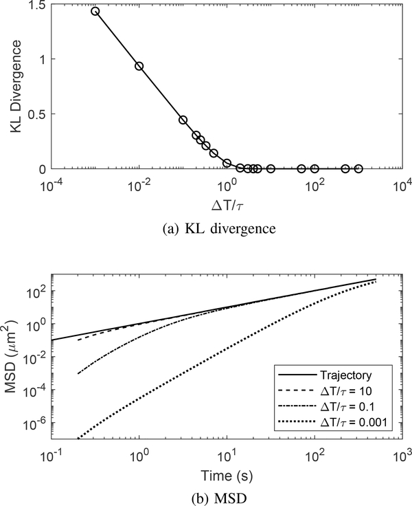
As only the relative time scale matters, we describe our results using the ratio $\frac{\mathrm{\Delta }T}{\tau }$ rather than the individual values. In these comparison simulations, the diffusion coefficient was fixed at D = 1 μm²/s. The results in terms of the KL divergence between the true Brownian motion SSPDF and that of the tracker system, as well as the MSD comparison, are shown in Fig. 4. At small values of the ratio $\frac{\mathrm{\Delta }T}{\tau }$, the KL divergence increases indicating that the SSPDF no longer matches that of the ideal Brownian motion. Once the ratio reaches unity, the KL divergence is essentially zero. At these large ratios, the time ΔT is large relative to the system time constant and thus the stage can settle to the reference position defined by the Brownian motion sample path. When viewed at the sampling points, then, the input and output trajectories look identical and the distributions match.

Fig. 4.

Tracker performance in terms of (a) KL divergence between the SSPDFs of a true Brownian motion and the tracker output and (b) the MSD.

For the MSD, Fig. 4 highlights three scenarios, ranging from small to large ratios of the time constants. All three cases converge to the ideal Brownian motion. However, the time it takes to converge varies and is longer for smaller $\frac{\mathrm{\Delta }T}{\tau }$. At the steady state condition, the stage motion MSD slope matches the desired one, indicating that the stage motion accurately reproduces the original motion in terms of MSD statistics (and, as noted above, in terms of KL divergence). In a practical implementation, this implies that the experiment should wait until the stage is at steady state before data collection starts.

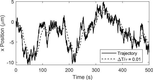
The temporal effects of small $\frac{\mathrm{\Delta }T}{\tau }$ values become readily apparent when the stage response is compared with the input Brownian motion trajectory, shown in Fig. 5. As expected, the low-pass nature of the stage dynamics filters out the highest frequency motions of the true Brownian motion sample path. This smoothing effect grows larger as the KL divergence grows larger. However, despite the filtering, the stage still follows the general shape of the trajectory preserving the MSD and MSD slope with minimal error. As the value of $\frac{\mathrm{\Delta }T}{\tau }$ continues to grow smaller, the stage has more difficulty following the general shape, resulting in larger initial errors in both the MSD and the MSD slope to occur and a longer transient period before the system settles to accurate statistics.

Fig. 5.

Sample path of a Brownian motion (solid line) and filtered by the stage dynamics (dashed line).

This effect can also be seen by looking at the SSPDF (data omitted for space reasons). At very small ratios $\frac{\mathrm{\Delta }T}{\tau }$ the stage has very little time to respond to the step input before a new step is applied. As a result the stage steps are very small since a new command is given while the system is still in the transient period and the distributions have a very small variance. As this ratio gets larger, so that ΔT is large relative to the system time constant τ, the stage has sufficient time to respond and the step size distribution approaches that of the true Brownian motion.

The previous simulations were done for a moderate diffusion constant of 1 μm²/s but did not explore the performance at different values of D. As it is reasonable to expect that the ability to faithfully represent trajectories of a given diffusion constant will depend on the time scale of the system, we simulated the system over a large range of both D and $\frac{\mathrm{\Delta }T}{\tau }$. The diffusion coefficient was varied from 10⁻⁶ – 10⁶ μm²/s, much larger than the expected range in biophysical phenomena, which are typically in the range 10⁻³ – 10² μm²/s. The KL divergence is insensitive to D, and the relationship of $\frac{\mathrm{\Delta }T}{\tau }$ follows what was previously seen in Fig. 4a. Similarly, the MSD slope follows the same trend as before, converging to the same slope as the pure diffusion after a transient period that depends on the ratio $\frac{\mathrm{\Delta }T}{\tau }$. These results indicate that it is possible to reproduce Brownian motion of any value of D within the limitations of the hardware, such as slew rate and saturation at the amplifiers limits. Even with a fast time step and a slow stage response, the stage still converges to the desired value of D after a period of time. However, in this range of values, the trajectory still deviates from the desired trajectory resulting in a large KL divergence.

B. Feed forward Model-Inverse Control

The results above tell two stories. The first is that if only the statistics of motion are of interest, then a piezo stage of any time constant and a sampling time of any value can be used with the only penalty to be paid being an initialization time while the statistics stabilize. The second, however, is that if accurate tracking of the trajectory is desired, then the stage should be as fast as possible. This can be done through effective feedback control of the stage, giving the closed loop plant the highest bandwidth possible given other constraints on the system. Here we highlight that this can be combined with feedforward methods, notably model inverse control, as shown in Fig. 2d. It is important to note that one challenge to this approach is that many piezo systems have non-minimum phase zeros, though this can be overcome with the appropriate choice of feedforward controller [12].

For simplicity here, we ignore any possible right-half plane zeros and took the simple continuous time model

$$F(s)=\frac{\tau s+1}{k\mathrm{\Delta }Ts+1}.$$ (9)

Using matched pole-zero mapping, this transfer function was translated into a discrete time transfer function

$$F(z)=\left(\frac{1-e^{-k}}{1-e^{-\frac{\mathrm{\Delta }T}{\tau }}}\right)\left(\frac{z-e^{-\frac{\mathrm{\Delta }T}{\tau }}}{z-e^{-k}}\right)$$ (10)

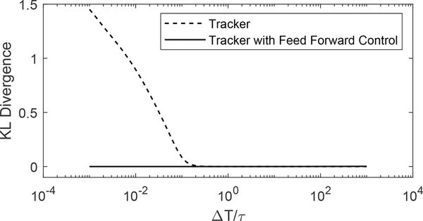
and included this in the Monte Carlo simulations. The parameter k in the feed-forward controller was included to tune the filter’s frequency response to allow balancing the stage error and the amplifier’s output to avoid saturation. In these simulations, the tuning parameter was set to k = 6. To compare the performance of the tracker with feedforward control to the plain tracker, we used the KL divergence as shown in Fig. 6. As expected, in the range where $\frac{\mathrm{\Delta }T}{\tau }\le 1$, the feedforward scheme shows an enormous improvement over the simpler tracker formulation. As $\frac{\mathrm{\Delta }T}{\tau }$ increases to the point where the dynamics of P are sufficiently fast, the difference between the two goes away. These results indicate that the use of feed forward may be a key element in producing the temporal resolution needed to reproduce the fastest trajectories accurately, allowing us to reproduce both fast diffusion as well as capturing motion blur.

Fig. 6.

KL divergence of both the tracker and tracker with feed forward model inverse control implemented

V. Conclusion

In this work we have explored through simulation the ability of a piezo actuated stage to faithfully recreate two different aspects of Brownian motion, the statistics and the detailed trajectory. Our results indicate that, when using an appropriate choice of implementation, the stage motion can accurately reflect the motion statistics for any diffusion coefficient independent of the time constant of the stage (subject only to practical limitations such as power, slew rate, and nonlinearities) after an initial transient period. For accurately producing the detailed trajectory, the time constant of the stage of course matters and here feed forward control can be used (in combination with feedback control) to push the stage bandwidth higher. Our results indicate that there is great potential in using piezo actuated stages to test and characterize SPT microscopes and algorithms with a known ground truth motion.

References

- [1].Chenouard N, Smal I, De Chaumont F, Maška M, Sbalzarini IF, Gong Y, Cardinale J, Carthel C, Coraluppi S, Winter M et al. , “Objective comparison of particle tracking methods,” Nature methods, vol. 11, no. 3, p. 281, 2014. [DOI] [PMC free article] [PubMed] [Google Scholar]
- [2].Cheezum MK, Walker WF, and Guilford WH, “Quantitative comparison of algorithms for tracking single fluorescent particles,” Biophysical journal, vol. 81, no. 4, pp. 2378–2388, 2001. [DOI] [PMC free article] [PubMed] [Google Scholar]
- [3].Moerner W, Shechtman Y, and Wang Q, “Single-molecule spectroscopy and imaging over the decades,” Faraday discussions, vol. 184, pp. 9–36, 2015. [DOI] [PMC free article] [PubMed] [Google Scholar]
- [4].Inoue S, Video microscopy. Springer Science Business Media, 2013. [Google Scholar]
- [5].Shaner NC, Steinbach PA, and Tsien RY, “A guide to choosing fluorescent proteins,” Nature methods, vol. 2, no. 12, p. 905, 2005. [DOI] [PubMed] [Google Scholar]
- [6].Giepmans BN, Adams SR, Ellisman MH, and Tsien RY, “The fluorescent toolbox for assessing protein location and function,” science, vol. 312, no. 5771, pp. 217–224, 2006. [DOI] [PubMed] [Google Scholar]
- [7].Ashley TT and Andersson SB, “A control law for seeking an extremum of a three-dimensional scalar potential field,” in American Control Conference (ACC), 2016 IEEE, 2016, pp. 6103–6108. [Google Scholar]
- [8].Ashley TT, Gan EL, Pan J, and Andersson SB, “Tracking single fluorescent particles in three dimensions via extremum seeking,” Biomedical optics express, vol. 7, no. 9, pp. 3355–3376, 2016. [DOI] [PMC free article] [PubMed] [Google Scholar]
- [9].Schilling RL and Partzsch L, Brownian motion: an introduction to stochastic processes. Walter de Gruyter GmbH & Co KG, 2014. [Google Scholar]
- [10].Papoulis A and Pillai SU, Probability, random variables, and stochastic processes. Tata McGraw-Hill Education, 2002. [Google Scholar]
- [11].Saxton MJ, “Modeling 2D and 3D Diffusion,” in Methods in Membrane Lipids. Totowa, NJ: Humana Press, 2007, pp. 295–321. [DOI] [PubMed] [Google Scholar]
- [12].Butterworth J, Pao L, and Abramovitch D, “Analysis and comparison of three discrete-time feedforward model-inverse control techniques for nonminimum-phase systems,” Mechatronics, vol. 22, no. 5, pp. 577–587, 2012. [Google Scholar]