Abstract
Positron emission tomography (PET) is an ill-posed inverse problem and suffers high noise due to limited number of detected events. Prior information can be used to improve the quality of reconstructed PET images. Deep neural networks have also been applied to regularized image reconstruction. One method is to use a pretrained denoising neural network to represent the PET image and to perform a constrained maximum likelihood estimation. In this work, we propose to use a generative adversarial network (GAN) to further improve the network performance. We also modify the objective function to include a data-matching term on the network input. Experimental studies using computer-based Monte Carlo simulations and real patient datasets demonstrate that the proposed method leads to noticeable improvements over the kernel-based and U-Net-based regularization methods in terms of lesion contrast recovery versus background noise trade-offs.
Keywords: Positron emission tomography, convolutional neural network, iterative reconstruction, generative adversarial network, kernel-based reconstruction, self-attention
1. Introduction
Positron emission tomography (PET) is a functional imaging modality that provides in vivo visualization of biochemical processes in the body (Cherry et al. 2012). However, PET images suffer from high noise due to the ill-posed nature of tomographic image reconstruction and low counting statistics of PET data.
In the early 1980s, maximum likelihood expectation maximization (MLEM) algorithms (Shepp and Vardi 1982, Lange et al. 1984) were proposed for PET reconstruction. However, maximum-likelihood (ML) methods suffered from excessive noise propagation from the measurements. To overcome this limitation, regularized image reconstruction methods (Mumcuoglu et al. 1994, Fessler 1994, Qi et al. 1999, Qi and Leahy 2000) were introduced to improve image quality. Regularization functions usually model prior information about PET images. For instance, the quadratic smoothness prior (Silverman et al. 1990) is used to encourage image voxels to be similar to their neighbours, but it tends to produce blurry images as it heavily penalizes edges in images. Non-quadratic priors (Nuyts et al. 2002, Ahn and Leahy 2008, Wang and Qi 2012) were proposed to preserve sharp edges. Although these image priors have proven to be useful, they are based on heuristically designed models which may not capture true prior information about PET image characteristics. An alternative is to find the appropriate signal models by learning from existing images. One example is the dictionary learning based image reconstruction approach (Xu et al. 2012, Chen et al. 2015). A set of over-complete basis functions or a dictionary could be learned either from existing images or adaptively during image reconstruction. Those models have been used to reconstruct images from low-dose or limited-view data. Another kind of learning-based regularization is the kernel method, which exploits prior information from co-registered anatomical images or dynamic PET scans (Wang and Qi 2015, Hutchcroft et al. 2016, Gong, Cheng-Liao, Wang, Chen, Catana and Qi 2018). Unfortunately, the kernel method cannot be applied to static PET image reconstruction when there is no patient-specific prior information available.
Over the past several years, machine learning (Jordan and Mitchell 2015), and especially the use of deep neural networks (LeCun et al. 2015), has dramatically improved the state-of-the-art in visual object recognition, object detection, and many other domains. These successes attracted tremendous attention and led to an explosion of research in the application of machine learning to medical image reconstruction (Wang et al. 2018, Ravishankar et al. 2019, Gong et al. 2020). Besides post-processing reconstructed images (Xu et al. 2017, Gong et al. 2019b), there are several ways in which deep neural networks (DNN) can be applied to image reconstruction, including direct inversion (Zhu et al. 2018, Häggström et al. 2019), image regularization (Kim et al. 2018, Wu et al. 2017), and network unrolling (which unrolls an iterative image reconstruction algorithm into a layer-wise structure and replaces certain components by neural networks) (Gregor and LeCun 2010, Sun et al. 2016). The approach of using a deep image prior (Ulyanov et al. 2018) has also been applied to PET reconstruction, where the image is regularized by the network structure and the network training is performed during the image reconstruction using the patient data alone (Gong, Catana, Qi and Li 2018, Cui et al. 2019, Hashimoto et al. 2019). To incorporate prior information from existing high-quality PET images, here we focus on the network-constrained image reconstruction method (Baikejiang et al. 2018, Gong et al. 2019a), where a denoising convolutional neural network (CNN), trained by high-quality images, is used to represent feasible PET images in a constrained maximum likelihood reconstruction framework. This approach can be considered as an extension of the kernel representation and dictionary learning methods. Since DNNs have higher capacity in representing PET images than simple penalty functions and patch-based dictionaries, it is expected that DNN-based regularization can improve PET image quality. Previously, we used a convolutional neural network (CNN) in network-constrained PET image reconstruction and demonstrated improved performance compared to a standalone, deep learning-based denoising method Gong et al. (2019a). However, training a CNN generally requires a large amount of training images. Furthermore, the simple loss functions that we had used previously, including the mean squared error (MSE) and mean absolute error (MAE), tend to produce blurry images (Mardani et al. 2019).
To address these issues, we propose to replace the original network with a generative adversarial network (GAN) (Goodfellow et al. 2014), which has achieved great success in various image generation tasks since its introduction. We can view GAN as a learned loss function that could in principal, perform previously unattainable tasks. By introducing the adversarial loss, GAN can produce denoised images that resemble high-count PET images more closely than denoised results using a CNN. We also introduce an extra likelihood function that encourages the network input to be similar to the unregularized ML reconstruction so that the output of the GAN is always based on a noisy PET image, in a spirit similar to the conditional GAN (Mirza and Osindero 2014). Preliminary results of this work were previously presented at the 2019 International Meeting on Fully Three-Dimensional Image Reconstruction in Radiology and Nuclear Medicine (Xie et al. 2019). This paper includes substantial new results with quantitative evaluations using computer-based Monte Carlo simulations and real patient datasets from two different PET scanners and compares the results with the kernel-based and CNN-based iterative reconstruction methods.
2. Methods
2.1. Formulation and optimization
PET data are well modeled as a collection of independent Poisson random variables. For M number of lines of response (LOR) and N number of image voxels, a typical PET imaging model could be expressed in the following matrix form:
| (1) |
where is the expectation vector for PET data, is the unknown radioactive tracer distribution, and is the detection probability matrix with the (i, j)th element pij being the probability of detecting a photon pair produced in voxel j by LOR i. and denote the expectations of scattered and random coincidences, respectively. The log-likelihood function for y can be written as
| (2) |
The maximum likelihood estimate of the unknown image x is then given by:
| (3) |
To improve the image quality and reduce noise, we use a pre-trained DNN to constrain the unknown PET image to the output range of the DNN (Gong et al. 2019a):
| (4) |
where denotes the DNN and α denotes the noisy input to the neural network. The network was trained by using MLEM reconstructions of low-count data as inputs and MLEM reconstructions of high-count data as labels. In the original paper (Gong et al. 2019a), the PET image was estimated by solving the following constrained maximum likelihood estimation problem:
| (5) |
Since the network input α is updated during the image reconstruction process, if that updated input does not match the noise level of the training images, there is a risk of not being able to recover the high-quality image by the network. To address this issue, we modify the objective function to include a data-match term on the network input and solve the following constrained optimization problem:
| (6) |
where η is a weighting factor that balances the two terms. The first term in the objective function encourages the network input α to match the projection data via the likelihood function. For this reason, we expect α to have a noise level similar to those in the training images. When we set η to 0, the modified objective function and the whole optimization process simplifies to the previous method (Gong et al. 2019a).
We use the augmented Lagrangian approach for the constrained optimization problem in (6):
| (7) |
which can be maximized by the alternating direction method of multipliers (ADMM) (Boyd et al. 2011) in three steps:
| (8) |
| (9) |
| (10) |
The second step in (9) can be further split it into two steps:
| (11) |
| (12) |
| (13) |
We solve equations (8) and (11) by the MAP-EM algorithm and equation (12) by a gradient ascent algorithm. The final update equations for pixel j are
| (14) |
| (15) |
| (16) |
| (17) |
| (18) |
where , and are obtained by the MLEM update as
| (19) |
| (20) |
and S = 0.01 is the step size. When η = 0, the optimization is the same as the one given in (Gong et al. 2019a).
2.2. The GAN Network
We propose a GAN network to replace the U-Net used previously (Gong et al. 2019a). Fig. 1(a) shows the structure of the GAN network. The input of the network consists of five consecutive slices of 128×128 low-count PET images and the output is a 128×128 denoised image corresponding to the middle slice of the input. The GAN network contains a generator, denoted by G, and a discriminator, denoted by D. The generator is trained to produce low-noise PET images that cannot be distinguished from real high-count PET images by the discriminator. We further include a self-attention module in the GAN framework (Zhang et al. 2018). The insertion of the self-attention gate follows the strategy proposed by Zhang et al. (Zhang et al. 2018). The self-attention module calculates response at a position as a weighted sum of the features at all positions, which enables the generator and the discriminator to efficiently model long range dependencies across the image region. Similar to the non-local means filter, models trained with a self-attention module implicitly learn to suppress irrelevant regions in an input image while highlighting salient features. Previous studies show that either U-net (Oktay et al. 2018) or GAN (Zhang et al. 2018) can benefit from a self-attention module. Readers are referred to references (Zhang et al. 2018, Oktay et al. 2018) for more information on the attention mechanism.
Figure 1:
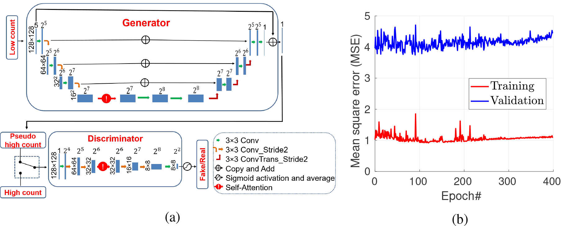
(a) The schematic of the self-attention GAN with U-net structure. (b) The training and validation mean square errors.
The training loss functions for the generator and discriminator are given by:
| (21) |
| (22) |
where α and x denote the low and high count images, respectively, lbce is the binary cross-entropy loss function (Wolterink et al. 2017), and λ is a weighting parameter. As shown in (21), a linear combination of adversarial losses and L2 loss is used to update the generator model so that the generator is trained to not only fool the discriminator but also make the expected output close to the target images.
The network of self-attention GAN (SAGAN) was in implemented in Tensorflow 1.6 and trained on an NVIDIA GTX 1080 Ti GPU. To improve the convergence of the network training, we pre-trained the generator for 100 epochs using the L2 loss function alone and then started the alternate training of the generator and discriminator. In order to choose the proper epoch number, the L2 losses of the training and validation datasets for each epoch were saved and are shown in Fig. 1 (b). For this specific dataset, we can see that the training loss was decreasing while the validation loss started to increase after 100 iterations. Note that training loss also slightly increases after 200 epochs because of the update of the discriminator. Considering the validation loss, the network trained by 100 epochs was saved for deployment. The trained network was used either as a denoising network (SAGAN-Den) or in the iterative reconstruction with either η = 0 (SAGAN-Iter-E0) and η = 0.5 (SAGAN-Iter-E0.5). The value of η = 0.5 was chosen empirically by balancing the two terms in the objective function in (6). Influence of different η values are discussed in Section 4.5.
3. Experimental evaluations
3.1. Simulation Study
Computer simulated data were first used to evaluate the proposed method following the same procedure described in (Gong et al. 2019a). The simulation modeled the geometry of a GE 690 scanner (Bettinardi et al. 2011). Twenty XCAT phantoms (Segars et al. 2010) with different organ sizes and genders were simulated. Eighteen phantoms were used for training, one was used for validation and one for testing. The image matrix size was 128×128×49 with 3.27 × 3.27 × 3.27 mm3 voxels. For the training data, thirty hot spheres with diameters ranging from 12.8 mm to 22.1 mm were inserted in the lung region. For the test phantom, two lesions with diameter 12.8 mm were inserted. The time activity curves of different tissues were generated using kinetic parameters mimicking 18F-FDG scan. The values of the parameters are given in (Gong et al. 2019a). The neural network was trained with low-count reconstructions (4-min scans) as input and high-count reconstructions (40-min scans) as labels. For quantitative comparisons, contrast recovery (CR) for inserted lesions vs. the background standard deviation (STD) curves were plotted. The CR was computed as
| (23) |
where R = 10 is the number of realizations, is the uptake of the lung lesion in realization r, and is true value of lesion uptake. The background STD was computed as
| (24) |
where br,k is the average value of the kth background ROI in the rth realization and Kb is the number of background ROIs in each image. Twenty 2D circular ROIs with a diameter of 16.4 mm were manually drawn in the uniform liver region across different axial slices to calculate the background STD values. The two-tailed paired t-test was used to examine the statistical significance of the noise reduction at matched CR levels.
3.2. Real patient study
Real patient datasets were acquired from two TOF-PET/CT scanners, a GE Discovery 690 (Bettinardi et al. 2011) (GE Healthcare, Waukesha, WI, USA) and Canon Celesteion (Kaneta et al. 2017) (Canon Medical Corporation, Tochigi, Japan).
3.2.1. Hybrid lesion dataset
Six female patients with breast cancer received one-hour 18F-FDG dynamic scans on the GE PET/CT scanner covering the thorax region. The injected activity ranged from 190 to 410 MBq and the body weights ranged from 45 to 112 (72.1±20.7) kg. Five of the datasets were used for training and one was reserved for testing. High-count data were obtained using the portion of the events from 20 to 60 minutes post injection and low-count data were generated by randomly down-sampling the high-count data to 1/10th events. For each training subject, ten realizations of the low-count datasets were generated by resampling the high-count data to increase the training data size. For each realization, additional data transformations including one random image translation and one rotation were used. The distribution of the horizontal and vertical translation offsets was uniform between −20 and 20 pixels. The rotation angle was uniformly distributed between 0 and 90 degrees clockwise. For the test subject, five realizations of the low-count datasets were generated to evaluate the noise performance. The low-count datasets were reconstructed using the ML-EM algorithm with 20, 30, and 50 iterations to account for different noise levels. The high-count dataset was reconstructed using the ML-EM algorithm with 50 iterations. The matrix size for the reconstructed images was 180 × 180 × 49 with a voxel size of 3.27 × 3.27 × 3.27 mm3.
For quantitative comparisons, spherical lesions were manually inserted into the validation data, but not into the training data. The inserted lesions were 13.1 mm and 16.4 mm in diameter and shared the same time activity curve (TAC) with a real breast lesion. Lesion CR vs. the background STD curves were plotted. Twenty 2D circular ROIs with a diameter of 16.4 mm were manually drawn in the liver region across different axial slices to calculate the background STD values.
3.2.2. Lung cancer dataset
The lung cancer dataset consisted of seven 18F-FDG patient scans acquired over two bed positions with 50% overlap. Each bed position was scanned for 14 min. The injected activity ranged from 160 to 250 MBq and the body weights of seven male patients ranged from 45 to 74 (62.1±8.8) kg. Five datasets were used for training, one for validation, and one for testing. The 14-min scans were used as the high-count dataset and the low-count dataset was obtained by down-sampling the high-count data to 1/7th of the events. The same data augmentation and reconstruction procedures described above were used. The matrix size for the reconstructed images was 272 × 272 × 141 with a voxel size of 2.0 × 2.0 × 2.0 mm3. Background ROIs were chosen in the liver region to calculate the STD. Since true lesion uptakes in real patient datasets were not known, we computed lesion contrast values instead of CR in the quantitative analysis. Lesion contrast is defined as:
| (25) |
where, and are the mean uptake of the lung lesion and the liver ROI in realization r respectively. Twenty 2D circular ROIs with a diameter of 16.4 mm were manually drawn in the uniform liver region across mutliple axial planes based on high-count PET images.
3.3. Reference Methods
We compared the proposed method with the kernel based reconstruction (Wang and Qi 2015) and the iterative CNN method published previously (Gong et al. 2019a). For the kernel based reconstruction, we used either the dynamic PET or CT image to generate the kernel matrix using the radial Gaussian kernel. Before feature extraction, both PET and CT images were normalized so that the image standard variation was 1.
For the dynamic PET kernel, each one-hour long dynamic PET dataset was rebinned into three twenty-minute frames and reconstructed using the MLEM algorithm to extract the feature vectors:
| (26) |
where , m = 1,2,3, are the three reconstructed images. Then the kernel matrix K was calculated by
| (27) |
where σ2 is the variance of the feature images and is the number of voxels in the dynamic PET feature vector. This method is referred to as KEMPET.
For CT guided kernel reconstruction, we generated the kernel matrix by
| (28) |
where μi is a local patch centered at voxel i from the co-registered CT image and is the number of voxels in the patch. This method is referred to as KEMCT.
In this paper, a 3×3×3 local patch was extracted for each voxel to form the feature vectors. and were 81 and 27, respectively. For efficient computation, all kernel matrices were constructed using a k-Nearest-Neighbor (kNN) search (Gong, Cheng-Liao, Wang, Chen, Catana and Qi 2018) in a 7×7×7 search window with k = 30. As shown in previous publications (Hutchcroft et al. 2016, Gong, Cheng-Liao, Wang, Chen, Catana and Qi 2018), the kernel-based method can achieve better image quality compared to MLEM with and without post-reconstruction denoising in low-count PET reconstructions.
For the iterative CNN method, we use the same U-Net structure shown in Fig. 1 (a), but without the attention gate. The network was trained using the same training data and the trained network was used either as a denoising network (Unet-Den) or in the iterative reconstruction (Unet-Iter).
4. Results
4.1. Simulation data
Fig. 2 shows, from top to bottom, transverse, coronal, and sagittal views of different reconstructed images. Comparing Figures 2 (b) and (c), we can see that the tumors in the lung region have higher contrast in the SAGAN denoised image than in the Gaussian filtered image. Myocardium boundary inside the heart is also sharper and more continuous in the SAGAN denoised image. Similar improvement patterns can also be seen between Fig. 2(b) and Fig. 2(d).
Figure 2:
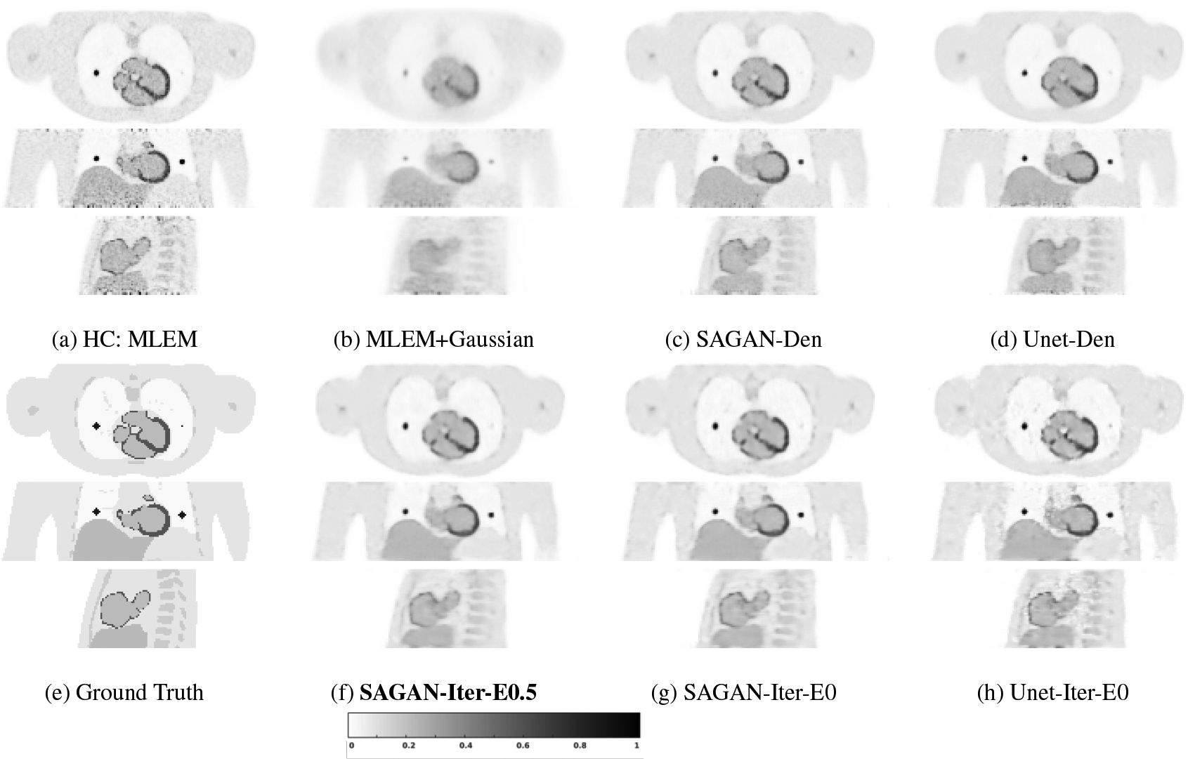
Reconstructed low-count images using different methods for the simulated test data set. The bold caption denotes our proposed method.
From the CR vs. STD curves shown in Fig. 3, we can see that the proposed iterative reconstruction with the SAGAN outperforms all the other methods with the highest CR at any matched STD level. At a matched CR level of 0.7, SAGAN-Iter-E0.5 result has significantly lower noise in the liver background than both SAGAN-Iter-E0 and Unet-Iter-E0 results with the associated p-values of p = 0.020 and p = 0.0061, respectively. We can also see that denoising performance of the SAGAN is better than the original U-Net, although the difference in the iterative reconstructions is much reduced. Including the new data term (SAGAN-Iter-E0.5) also improves the lesion CR slightly over the case with η = 0.
Figure 3:
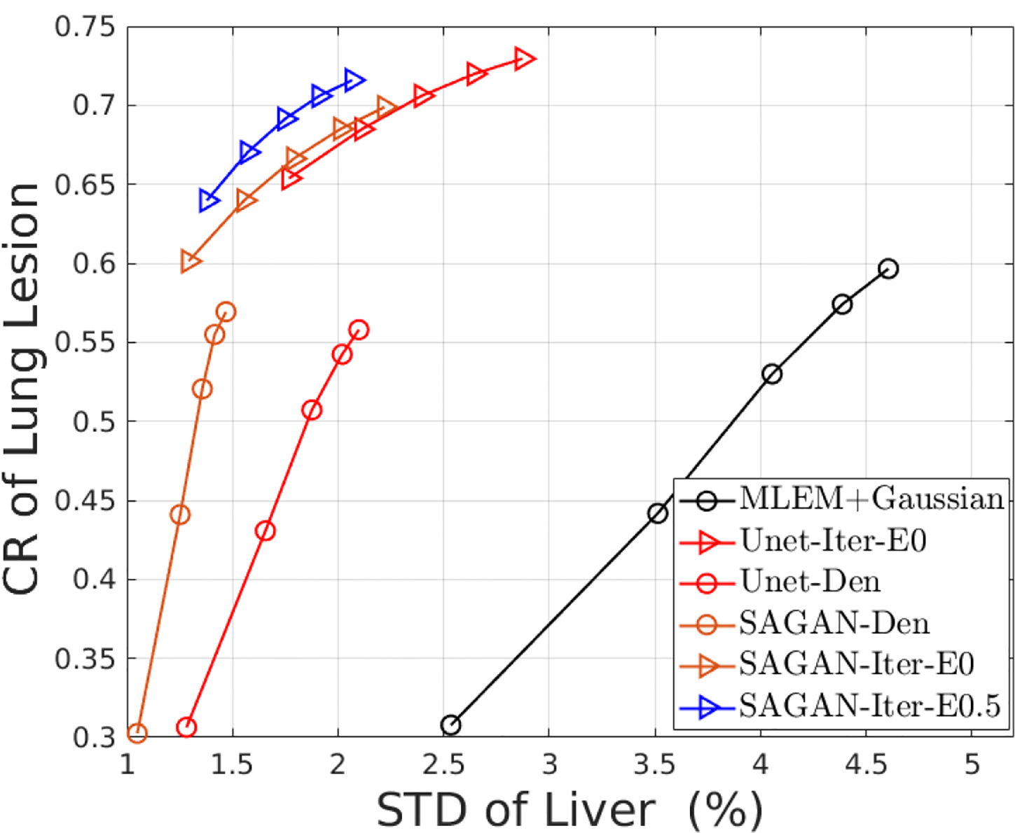
The contrast recovery versus standard derivation curves using different methods for the simulated test data set.
4.2. Hybrid lesion data
Fig. 4 shows transverse, coronal, and sagittal views of different reconstructed images. The CR vs. STD curves are shown in Fig. 5 (a). In comparison, MLEM has the worst performance and the SAGAN based iterative method holds the best CR-STD trade-off among all the methods. After introducing the extra data term (η = 0.5), SAGAN-iterative-Eta0.5 converges faster and achieves a slightly better performance than the case with η = 0 (SAGAN-iterative-Eta0). Moreover, compared with the denoising approaches, integrating the neural networks in the iterative reconstruction framework takes the data consistency into consideration and can recover more image details. Also while the directly denoised images by the U-Net and SAGAN have quite different CR for the lung lesion, the regularized reconstruction methods using the two networks respectively obtained similar contrast recovery. Finally, Fig. 5 (b) demonstrates the proposed SAGAN-regularized reconstruction can achieve similar or better performance than the two kernel methods without using any patient specific prior information.
Figure 4:
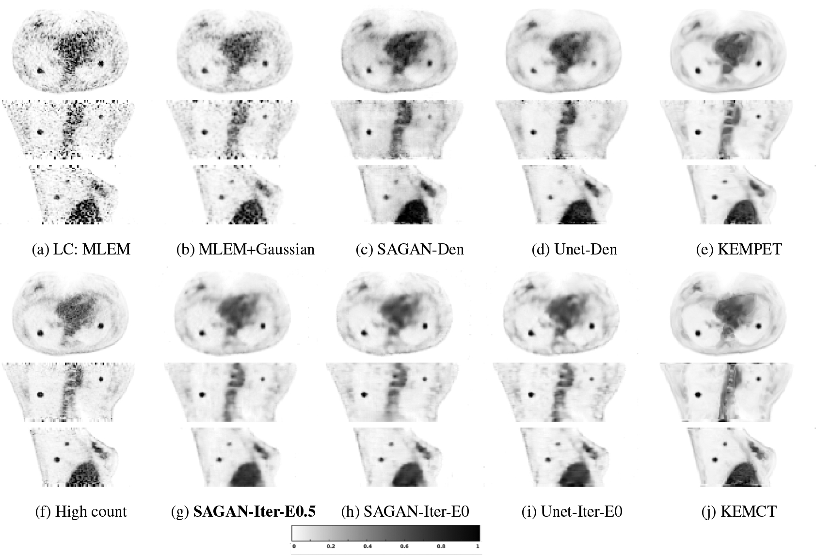
Reconstructed low-count images using different methods for the hybrid lesion test dataset. The bold caption denotes our proposed method.
Figure 5:
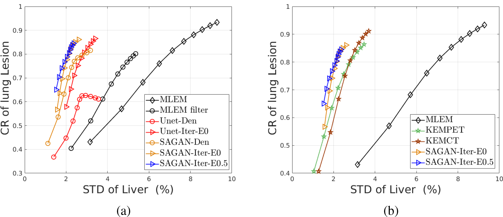
The contrast recovery versus standard derivation curves using different methods for the hybrid lesion test dataset.(a) The comparison between the SAGAN and U-net structures. (b) The comparison between SAGAN-based and kernel-based reconstruction.
4.3. Lung cancer patient data
Fig. 6 shows the reconstructed images and Fig. 7 shows the lesion contrast vs. STD curves for the lung cancer test dataset. Comparing the different denoising methods, we can see that the tumors in the lung region have higher contrast in the SAGAN denoised image (Fig. 6 (c)) than in the Gaussian filtered image (Fig. 6 (b)). Moreover, SAGAN produces higher lesion contrast and has higher levels of noise tolerance than the U-net as shown in Fig. 7. Similar to the results of hybrid lesion data, we also find that the tumor contrasts are higher in the network-regularized reconstructions compared to their denoising counterparts. Integrating DNNs in the reconstruction also reduces the difference between U-Net and SAGAN in terms of CR. From Fig. 7, we can see that the extra data term (η = 0.5) provides a slight improvement in lesion contrast, although the benefit is smaller in this dataset.
Figure 6:
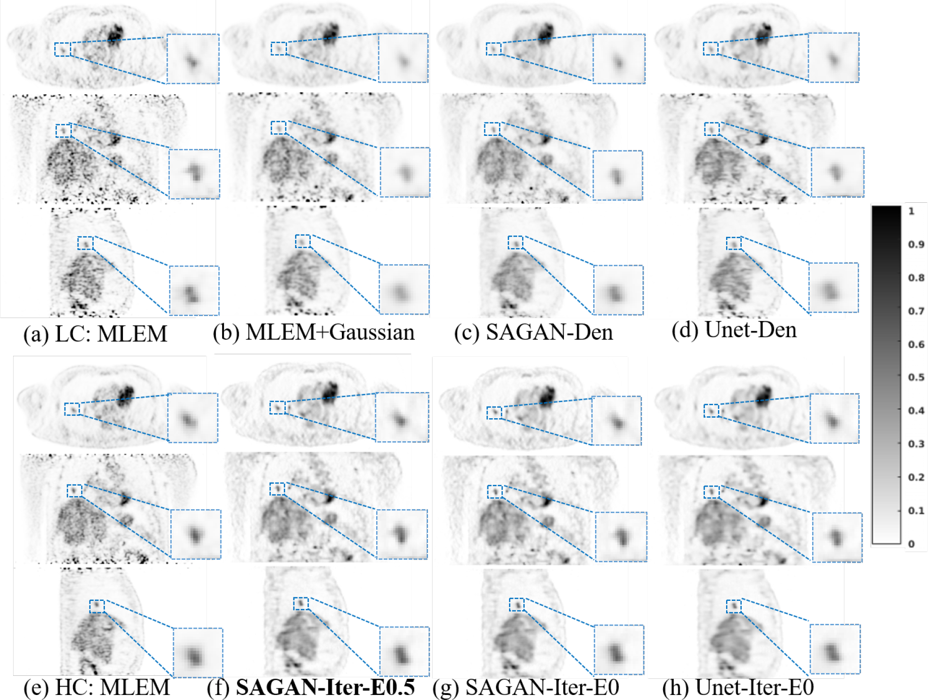
Reconstructed low-counts images using different methods for the lung cancer test dataset. The bold caption denotes our proposed method.
Figure 7:
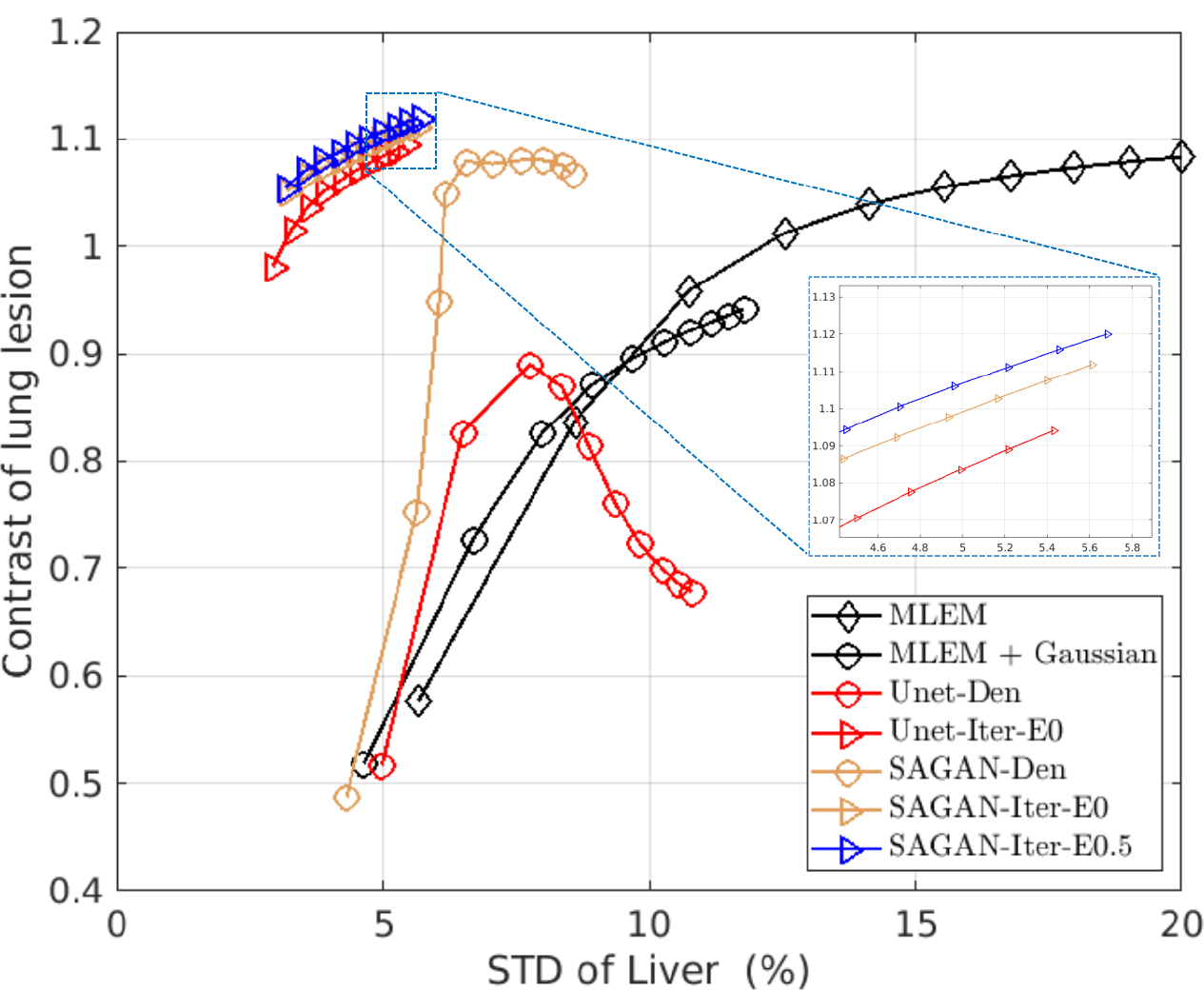
The contrast versus standard derivation curves using different methods for the lung cancer test dataset.
4.4. Computation time
For deep learning based methods, the main computational cost comes from the training stage. Although the training is done on GPUs, it is still time-consuming. For the hybrid lesion dataset, which contains 6,125 slices of 2D images, the training times of the U-net and proposed SAGAN are 1.6 min and 3.8 min per epoch, respectively. The kernel-based methods (KEMCT and KEMPET) do not require a training phase, but they took 8 min to build a patient specific kernel matrix. Once the network is trained offline, the deep learning based methods are much more efficient than KEMCT or KEMPET in terms of the model building time for a new patient. For reconstruction, the average execution times (CPU mode) of each iteration of MLEM, KEMCT/KEMPET, SAGAN-Iter-E0/Unet-Iter-E0, and SAGAN-Iter-E0.5 were 0.65, 0.7, 0.81 and 0.9 min, respectively, for the hybrid lesion dataset. The major computation time is in the forward and back projection operations, which used a precomputed system matrix based on multi-ray tracing to model the crystal penetration effect (Huesman et al. 2000). The reconstruction time can be accelerated by using a factored system matrix (Zhou and Qi 2011, 2014). Another time consuming part is the switching between the image update, which was implemented in Matlab, and the deep network update, which was implemented in Tensorflow. This can be avoided by implementing the forward and back projections in Tensorflow in the future.
4.5. Effect of η value
Based on the generative adversarial network, we proposed a framework for including a soft constraint on the network input during PET reconstruction. To investigate the effect of the soft constraint, we plotted the log-likelihood of the network input in Fig. 8. We can see that L(y|Pα + s + r) of SAGAN-iterative-Eta0 is decreasing over iterations, meaning that the noise level of the network input is unlikely to match that of the training images at the same iteration. In this case, the pre-trained network may generate undesirable outputs. After adding the soft constraint, an increase of L(y|Pα + s + r) can be observed for SAGAN-iterative-Eta0.5. It shows that the additional data term can help reduce the difference between the network inputs during reconstruction and training. Therefore, including the extra term in the SAGAN iterative reconstruction is highly recommended, even though the improvement is small in some test cases. Additionally, it shows that a larger η value results in a higher value of L(y|Pα + s + r) at later iterations, but also a lower value of L(y|Px + s + r). To balance these two terms, we empirically chose η = 0.5 in this study.
Figure 8:
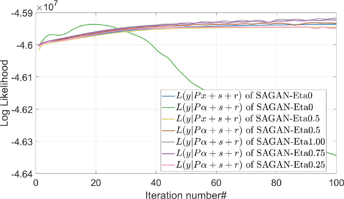
The effect of parameter η on the log-likelihood.
5. Discussion
In this paper, we applied GAN to regularized PET image reconstruction. Previously, researchers had focused on using GAN to synthesize high quality medical images or directly denoised images (Yang et al. 2017, 2018, Ouyang et al. 2019). Our experimental results showed that the SAGAN outperformed the previous network, U-Net, in the datasets under comparison. One reason for the improvement is that MSE and MAE loss functions used in the previous network tend to produce blurry images. As an alternative, perceptual loss (feature loss in high dimensional space) (Johnson et al. 2016) can be used to enhance the image appearance. Similarly, structural similarity loss can suppress the over-smoothing behavior. Different levels of features can be chosen to determine whether they focus on local information such as edges, mid-level features such as textures or high-level features corresponding to global information. By incorporating perceptual loss, the network may have the potential to generate more realistic textures and details. However, it remains unclear how to select feature loss. In comparison, adversarial loss is a divergence-like measure between the true data distribution and the data distribution produced by the generator. The adversarial model encourages the generator outputs to be statistically indistinguishable from ground truth and does not require an explicit perception model.
Furthermore, the proposed SAGAN-regularized reconstruction can achieve better STD performance compared with two kernel methods without requiring a dynamic scan or CT images. In the hybrid data set, we artificially inserted tumors in both CT and PET images. Due to the perfect registration between PET and CT, KEMCT shows the highest CR. However, perfect registration is not possible in practice and CT and PET images may not have the same lesion boundaries. Therefore the proposed SAGAN regularized reconstruction, which does not require any patient specific prior information, is more promising.
Finally, the limitation of the 2D convolution layers we used in the SAGAN should be noticed. Since the SAGAN inevitably requires more GPU memory than the U-Net, we implemented 2D convolutions instead of 3D convolutions that we had used in previous work (Gong et al. 2019a). In the coronal or sagittal views of Fig. 6, some axial artifacts can be noticed in the arm region, even though we used five adjacent transaxial slices as the network input. It is possible to mitigate the axial artifacts and further improve the performance by using 3D CNN-based networks, which we will explore in the future.
6. Conclusion
In this work, we proposed a SAGAN-regularized PET image reconstruction method. Compared with the kernel methods, the new method does not require any patient specific prior information and uses only the population training pairs. Evaluations using computer simulations and real datasets indicate that the SAGAN-based regularization improves image quality and produces a better lesion CR vs. background STD trade-off curve than existing methods, including EM reconstruction with Gaussian filtering, kernel-based reconstruction and U-Net-regularized iterative reconstruction.
Acknowledgments
This work is supported by the National Institutes of Health under Grant R01EB000194 and R21EB026668.
References
- Ahn S and Leahy RM 2008. Analysis of resolution and noise properties of nonquadratically regularized image reconstruction methods for pet IEEE transactions on medical imaging 27(3), 413–424. [DOI] [PubMed] [Google Scholar]
- Baikejiang R, Gong K, Zhang X and Qi J 2018. An improved deep learning based regularized image reconstruction for PET IEEE Nuclear Science Symposium and Medical Imaging Conference (NSS/MIC). [Google Scholar]
- Bettinardi V, Presotto L, Rapisarda E, Picchio M, Gianolli L and Gilardi M 2011. Physical performance of the new hybrid PET/CT Discovery-690 Medical physics 38(10), 5394–5411. [DOI] [PubMed] [Google Scholar]
- Boyd S, Parikh N, Chu E, Peleato B, Eckstein J et al. 2011. Distributed optimization and statistical learning via the alternating direction method of multipliers Foundations and Trends in Machine learning 3(1), 1–122. [Google Scholar]
- Chen S, Liu H, Shi P and Chen Y 2015. Sparse representation and dictionary learning penalized image reconstruction for positron emission tomography. Physics in Medicine and Biology 60(2), 807–23. [DOI] [PubMed] [Google Scholar]
- Cherry SR, Sorenson JA and Phelps ME 2012. Physics in nuclear medicine Elsevier Health Sciences. [Google Scholar]
- Cui J, Gong K, Guo N, Wu C, Meng X, Kim K, Zheng K, Wu Z, Fu L, Xu B et al. 2019. PET image denoising using unsupervised deep learning European journal of nuclear medicine and molecular imaging 46(13), 2780–2789. [DOI] [PMC free article] [PubMed] [Google Scholar]
- Fessler JA 1994. Penalized weighted least-squares image reconstruction for positron emission tomography IEEE Transactions on Medical Imaging 13(2), 290–300. [DOI] [PubMed] [Google Scholar]
- Gong K, Berg E, Cherry SR and Qi J 2020. Machine learning in pet: From photon detection to quantitative image reconstruction Proceedings of the IEEE 108(1), 51–68. [DOI] [PMC free article] [PubMed] [Google Scholar]
- Gong K, Catana C, Qi J and Li Q 2018. PET image reconstruction using deep image prior IEEE transactions on medical imaging 38(7), 1655–1665. [DOI] [PMC free article] [PubMed] [Google Scholar]
- Gong K, Cheng-Liao J, Wang G, Chen KT, Catana C and Qi J 2018. Direct patlak reconstruction from dynamic PET data using kernel method with mri information based on structural similarity IEEE transactions on medical imaging 37(4), 955–965. [DOI] [PMC free article] [PubMed] [Google Scholar]
- Gong K, Guan J, Kim K, Zhang X, Yang J, Seo Y, El Fakhri G, Qi J and Li Q 2019a. Iterative PET image reconstruction using convolutional neural network representation IEEE transactions on medical imaging 38(3), 675–685. [DOI] [PMC free article] [PubMed] [Google Scholar]
- Gong K, Guan J, Liu C and Qi J 2019b. PET image denoising using a deep neural network through fine tuning IEEE Transactions on Radiation and Plasma Medical Sciences 3(2), 153–161. [DOI] [PMC free article] [PubMed] [Google Scholar]
- Goodfellow I, Pouget-Abadie J, Mirza M, Xu B, Warde-Farley D, Ozair S, Courville A and Bengio Y 2014. Generative adversarial nets in ‘Advances in neural information processing systems’ pp. 2672–2680. [Google Scholar]
- Gregor K and LeCun Y 2010. Learning fast approximations of sparse coding in ‘Proceedings of the 27th International Conference on International Conference on Machine Learning’ Omnipress pp. 399–406. [Google Scholar]
- Häggström I, Schmidtlein CR, Campanella G and Fuchs TJ 2019. Deeppet: A deep encoder–decoder network for directly solving the pet image reconstruction inverse problem Medical image analysis 54, 253–262. [DOI] [PMC free article] [PubMed] [Google Scholar]
- Hashimoto F, Ohba H, Ote K, Teramoto A and Tsukada H 2019. Dynamic PET image denoising using deep convolutional neural networks without prior training datasets IEEE Access 7, 96594–96603. [Google Scholar]
- Huesman RH, Klein GJ, Moses WW, Qi J, Reutter BW and Virador PR 2000. List-mode maximum-likelihood reconstruction applied to positron emission mammography (pem) with irregular sampling IEEE transactions on medical imaging 19(5), 532–537. [DOI] [PubMed] [Google Scholar]
- Hutchcroft W, Wang G, Chen KT, Catana C and Qi J 2016. Anatomically-aided PET reconstruction using the kernel method Physics in Medicine and Biology 61(18), 6668. [DOI] [PMC free article] [PubMed] [Google Scholar]
- Johnson J, Alahi A and Fei-Fei L 2016. Perceptual losses for real-time style transfer and super-resolution in ‘European conference on computer vision’ Springer pp. 694–711. [Google Scholar]
- Jordan MI and Mitchell TM 2015. Machine learning: Trends, perspectives, and prospects Science 349(6245), 255–260. [DOI] [PubMed] [Google Scholar]
- Kaneta T, Ogawa M, Motomura N, Iizuka H, Arisawa A, Yoshida K and Inoue T 2017. Initial evaluation of the celesteion large-bore PET/CT scanner in accordance with the NEMA NU2–2012 standard and the Japanese guideline for oncology FDG PET/CT data acquisition protocol version 2.0 EJNMMI research 7(1), 83. [DOI] [PMC free article] [PubMed] [Google Scholar]
- Kim K, Wu D, Gong K, Dutta J, Kim JH, Son YD, Kim HK, El Fakhri G and Li Q 2018. Penalized pet reconstruction using deep learning prior and local linear fitting IEEE transactions on medical imaging 37(6), 1478–1487. [DOI] [PMC free article] [PubMed] [Google Scholar]
- Lange K, Carson R et al. 1984. Em reconstruction algorithms for emission and transmission tomography J Comput Assist Tomogr 8(2), 306–16. [PubMed] [Google Scholar]
- LeCun Y, Bengio Y and Hinton G 2015. Deep learning nature 521(7553), 436. [DOI] [PubMed] [Google Scholar]
- Mardani M, Gong E, Cheng JY, Vasanawala SS, Zaharchuk G, Xing L and Pauly JM 2019. Deep generative adversarial neural networks for compressive sensing mri IEEE Transactions on Medical Imaging 38(1), 167–179. [DOI] [PMC free article] [PubMed] [Google Scholar]
- Mirza M and Osindero S 2014. Conditional generative adversarial nets arXiv preprint arXiv:1411.1784 [Google Scholar]
- Mumcuoglu EU, Leahy R, Cherry SR and Zhou Z 1994. Fast gradient-based methods for bayesian reconstruction of transmission and emission pet images. IEEE Transactions on Medical Imaging 13(4), 687–701. [DOI] [PubMed] [Google Scholar]
- Nuyts J, Beque D, Dupont P and Mortelmans L 2002. A concave prior penalizing relative differences for maximum-a-posteriori reconstruction in emission tomography IEEE Transactions on nuclear science 49(1), 56–60. [Google Scholar]
- Oktay O, Schlemper J, Folgoc LL, Lee M, Heinrich M, Misawa K, Mori K, McDonagh S, Hammerla NY, Kainz B et al. 2018. Attention u-net: Learning where to look for the pancreas arXiv preprint arXiv:1804.03999 [Google Scholar]
- Ouyang J, Chen KT, Gong E, Pauly J and Zaharchuk G 2019. Ultra-low-dose pet reconstruction using generative adversarial network with feature matching and task-specific perceptual loss Medical Physics 46(8), 3555–3564. URL: https://aapm.onlinelibrary.wiley.com/doi/abs/10.1002/mp.13626 [DOI] [PMC free article] [PubMed] [Google Scholar]
- Qi J and Leahy RM 2000. Resolution and noise properties of map reconstruction for fully 3-d PET Medical Imaging IEEE Transactions on 19(5), 493–506. [DOI] [PubMed] [Google Scholar]
- Qi J, Leahy RM, Cherry SR, Chatziioannou A and Farquhar TH 1999. High-resolution 3d bayesian image reconstruction using the micropet small-animal scanner Physics in Medicine and Biology 43(4), 1001–13. [DOI] [PubMed] [Google Scholar]
- Ravishankar S, Ye JC and Fessler JA 2019. Image reconstruction: From sparsity to data-adaptive methods and machine learning Proceedings of the IEEE pp. 1–24. [DOI] [PMC free article] [PubMed] [Google Scholar]
- Segars W, Sturgeon G, Mendonca S, Grimes J and Tsui BM 2010. 4d xcat phantom for multimodality imaging research Medical physics 37(9), 4902–4915. [DOI] [PMC free article] [PubMed] [Google Scholar]
- Shepp LA and Vardi Y 1982. Maximum likelihood reconstruction for emission tomography IEEE transactions on medical imaging 1(2), 113–122. [DOI] [PubMed] [Google Scholar]
- Silverman B, Jones M, Wilson J and Nychka D 1990. A smoothed em approach to indirect estimation problems, with particular reference to stereology and emission tomography Journal of the Royal Statistical Society: Series B (Methodological) 52(2), 271–303. [Google Scholar]
- Sun J, Li H, Xu Z et al. 2016. Deep admm-net for compressive sensing mri in ‘Advances in neural information processing systems’ pp. 10–18. [Google Scholar]
- Ulyanov D, Vedaldi A and Lempitsky V 2018. Deep image prior in ‘Proceedings of the IEEE Conference on Computer Vision and Pattern Recognition’ pp. 9446–9454. [Google Scholar]
- Wang G and Qi J 2012. Penalized likelihood pet image reconstruction using patch-based edge-preserving regularization IEEE transactions on medical imaging 31(12), 2194–2204. [DOI] [PMC free article] [PubMed] [Google Scholar]
- Wang G and Qi J 2015. PET image reconstruction using kernel method IEEE Transactions on Medical Imaging 34(1), 61–71. [DOI] [PMC free article] [PubMed] [Google Scholar]
- Wang G, Ye JC, Mueller K and Fessler JA 2018. Image reconstruction is a new frontier of machine learning IEEE transactions on medical imaging 37(6), 1289–1296. [DOI] [PubMed] [Google Scholar]
- Wolterink JM, Leiner T, Viergever MA and Išgum I 2017. Generative adversarial networks for noise reduction in low-dose CT IEEE Transactions on Medical Imaging 36(12), 2536–2545. [DOI] [PubMed] [Google Scholar]
- Wu D, Kim K, El Fakhri G and Li Q 2017. Iterative low-dose ct reconstruction with priors trained by artificial neural network IEEE transactions on medical imaging 36(12), 2479–2486. [DOI] [PMC free article] [PubMed] [Google Scholar]
- Xie Z, Baikejiang R, Gong K, Zhang X and Qi J 2019. Generative adversarial networks based regularized image reconstruction for PET in ‘15th International Meeting on Fully Three-Dimensional Image Reconstruction in Radiology and Nuclear Medicine’ Vol. 11072 International Society for Optics and Photonics; p. 110720P. [Google Scholar]
- Xu J, Gong E, Pauly J and Zaharchuk G 2017. 200x low-dose pet reconstruction using deep learning arXiv preprint arXiv:1712.04119 [Google Scholar]
- Xu Q, Yu H, Mou X, Zhang L, Hsieh J and Wang G 2012. Low-dose x-ray ct reconstruction via dictionary learning. IEEE Transactions on Medical Imaging 31(9), 1682–1697. [DOI] [PMC free article] [PubMed] [Google Scholar]
- Yang G, Yu S, Dong H, Slabaugh G, Dragotti PL, Ye X, Liu F, Arridge S, Keegan J, Guo Y et al. 2017. Dagan: deep de-aliasing generative adversarial networks for fast compressed sensing mri reconstruction IEEE transactions on medical imaging 37(6), 1310–1321. [DOI] [PubMed] [Google Scholar]
- Yang Q, Yan P, Zhang Y, Yu H, Shi Y, Mou X, Kalra MK, Zhang Y, Sun L and Wang G 2018. Low-dose ct image denoising using a generative adversarial network with wasserstein distance and perceptual loss IEEE transactions on medical imaging 37(6), 1348–1357. [DOI] [PMC free article] [PubMed] [Google Scholar]
- Zhang H, Goodfellow I, Metaxas D and Odena A 2018. Self-attention generative adversarial networks arXiv preprint arXiv:1805.08318 [Google Scholar]
- Zhou J and Qi J 2011. Fast and efficient fully 3D PET image reconstruction using sparse system matrix factorization with GPU acceleration Physics in Medicine and Biology 56(20), 6739. [DOI] [PMC free article] [PubMed] [Google Scholar]
- Zhou J and Qi J 2014. Efficient fully 3d list-mode tof pet image reconstruction using a factorized system matrix with an image domain resolution model Physics in Medicine and Biology 59(3), 541. [DOI] [PMC free article] [PubMed] [Google Scholar]
- Zhu B, Liu JZ, Cauley SF, Rosen BR and Rosen MS 2018. Image reconstruction by domain-transform manifold learning Nature 555(7697), 487. [DOI] [PubMed] [Google Scholar]


