

Excitable waves evolve into standing patterns and lead to the various dynamic and static protrusions seen in migrating cells.
Abstract
The mechanisms regulating protrusions during amoeboid migration exhibit excitability. Theoretical studies have suggested the possible coexistence of traveling and standing waves in excitable systems. Here, we demonstrate the direct transformation of a traveling into a standing wave and establish conditions for the stability of this conversion. This theory combines excitable wave stopping and the emergence of a family of standing waves at zero velocity, without altering diffusion parameters. Experimentally, we show the existence of this phenomenon on the cell cortex of some Dictyostelium and mammalian mutant strains. We further predict a template that encompasses a spectrum of protrusive phenotypes, including pseudopodia and filopodia, through transitions between traveling and standing waves, allowing the cell to switch between excitability and bistability. Overall, this suggests that a previously-unidentified method of pattern formation, in which traveling waves spread, stop, and turn into standing waves that rearrange to form stable patterns, governs cell motility.
INTRODUCTION
Excitable waves have been observed in various physiological settings, from rotating calcium waves in the cardiac myocyte (1) to actin polymerization waves during amoeboid cell migration (2). The wavefront in an excitable medium is created by a nonlinear activator response to a suprathreshold stimulus. This ultrasensitive response is all-or-none type, ensuring similar wave amplitudes across the medium. The wave back is formed by a down-jump in the activator owing to a delayed inhibitor response. The slow nature of the inhibitor creates an ensuing refractory period before the inhibitor returns to equilibrium, isolating an activity spike from subsequent triggers. Through diffusion, this spike propagates across adjacent excitable elements, creating a traveling wave.
In systems with only activator diffusion, the delayed inhibition allows the wave to spread without restriction in space, as is characteristic of neural waves (3). In contrast, interesting spatial phenomenon emerges with a diffusive inhibitor (4). For example, if the ratio of inhibitor to activator diffusion, δ ∼ 1, then one obtains diverse wave patterns, as in the Belousov-Zhabotinsky reaction (5). For δ » 1, lateral inhibition allows the formation of stable standing waves (6), creating patterns similar to many seen in nature, like the intricate involutions of seashells (7) or the tentacle patterns of Hydra (8). Theoretical studies demonstrate that it is possible for traveling and standing waves to coexist by altering the inhibitor diffusion, stalling traveling waves at the zero-velocity mark, leading to the emergence of standing waves (9).
In this study, we show how a direct transformation from a traveling to a standing wave can occur without changing diffusion parameters. In this case, zero wave speed or wave stopping is achieved through the natural accumulation of the inhibitor in space (10), similar to the wave-pinning mechanism proposed for bistable systems (11), thus allowing the system to move from an initially low equilibrium to a permanent higher stable state. This is achieved at intermediate levels of δ where traveling waves can also be sustained. Because alteration of diffusion coefficients is challenging, to the best of our knowledge, this direct transformation has not been demonstrated experimentally.
Our interest in this mechanism arose from recent observations of wave propagation in perturbed amoeboid cells (10, 12). Both excitable (13) and bistable systems (14) have been proposed to account for cellular protrusions during migration. The conflicting arguments regarding the roles of excitability and bistability in regulating protrusive morphology stems mostly from the fact that while some protrusions, such as the filopodium or the stable front in directed migration, cannot be explained by transient traveling waves (15), others, such as the signaling waves that are continually observed on the cell cortex, cannot arise from persistent activity that is typical of bistable systems. While in our earlier work we described how an excitable system model can reproduce different traveling wave phenotypes (10), we did not consider persistent protrusive activity. Here, we illustrate that a transformation from a traveling to a standing wave allows excitability and bistability to switch between one another without drastically altering system parameters. This allows us to explain the various types of cell protrusions seen in migrating cells and create an all-encompassing protrusive template. Moreover, in the process, we describe a potentially previously unknown method of pattern formation.
RESULTS
Traveling waves can transform into standing waves at the instant of wave stopping
The model we use to generate wave propagation (4, 16) is inspired by the FitzHugh-Nagumo model of excitability (17, 18), modified to ensure that the species levels remain positive. It consists of an autocatalytic activator (u) and a delayed inhibitor (v).
The ultrasensitivity of the activator manifests through the cooperativity term, while the delay in the inhibitor is incorporated through the variable ε, resulting in a time scale separation between the two components, creating a distinguishable wave “front” and “back.”
In phase-plane diagrams, the activator nullcline displays an inverted “N-shape” (fig. S1A). As the slope of the inhibitor nullcline is varied, the system undergoes two Hopf bifurcations, approximately at the minimum and maximum of the activator nullcline (19). Between these two bifurcation points, the equilibrium is unstable. The initial equilibrium is to the left of the minimum (fig. S1A) such that the threshold of the system corresponds approximately to the vertical distance between the equilibrium set point (v0) and the minimum of the activator nullcline (vmin) (19). Changes in r reflect external stimuli that lower the threshold of the system and trigger a large-scale excursion in phase space, which translates to a sharp up-jump in activity, thus creating the wavefront (fig. S1A).
This activator-inhibitor model has been used to recreate traveling waves observed on the cell cortex in different cell types (20–22). Our recent work has also suggested models for the underlying biochemical signaling network that displays this type of activator-inhibitor dynamics (10, 23). Using this model, we have shown how different wave characteristics are altered when perturbations are introduced to the governing signaling network, and that these model parameters allow us to capture a spectrum of traveling wave phenotypes.
The velocity of the excitable wavefront has been the subject of extensive research using singular perturbation approaches (3). In one-dimensional space, the wave velocity can be completely determined by a function of the initial level of the inhibitor, also called the controller species (24). This function is inversely proportional to v0, i.e., higher thresholds lead to slower wave velocities and vice versa.
The wave speed and wave stopping play a crucial role in determining the protrusive phenotype of cells (13). Specifically, how far the wave travels before extinguishing determines the wave range and, in turn, the size of the protrusion. If the dispersion of the inhibitor exceeds that of the activator, then, as a wave travels, the threshold levels continually increase in the surrounding, causing the wave to slow down as it spreads (10), ultimately stopping when a critical threshold is reached (Fig. 1A). Note that this stopping is independent of the size of the simulation domain (fig. S1E). This is similar to the wave-pinning mechanism (11), with the key difference being that the wave is extinguished upon stopping, instead of being pinned at a higher steady state that exists only in a bistable system. However, as we show below, it is possible for an initially low-equilibrium excitable system to spread as a traveling wave before switching to a higher-equilibrium steady state at the instant of wave stopping.
Fig. 1. Transformation of a traveling to a standing wave.
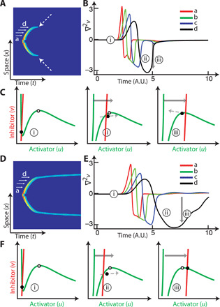
(A) Kymograph of a wave that traveled, stopped, and extinguished (c2 = 4.2 in inhibitor equation). Dashed arrows indicate where the stopping occurred. (B) Time profiles of a to d from the kymograph in (A), plotting the Laplacian evolution at each of these spatial points. (C) Illustration of how the nullclines are altered by the Laplacian term. The three situations correspond to the time instants marked in (B). The white circle denotes a bifurcation point; the equilibrium is stable if the inhibitor nullcline (red) is to the right of this. The black circle denotes the state, with the immediate trajectory shown by the dashed arrow. (D to F) Example of a standing wave. The panels are as in (A) to (C) but for a wave that transformed into a standing wave on stopping (c2 = 3.9 in inhibitor equation).
When a wave is triggered, the spatial gradient in inhibition makes the contribution of the diffusion term negative. Rewriting the inhibitor equation
we see that when the Laplacian is negative, the inhibitor nullcline shifts to the right and thereby lowers the threshold (Fig. 1, B and C). As the state moves around its trajectory, this gradient gradually subsides. If this shift is sufficiently large, then a new, stable, higher equilibrium is transiently created. This new equilibrium may attract the trajectory of the system, in which case the state remains at its new high state (Fig. 1, D to F, and movie S1). From the equation above, it is clear that a sufficiently large shift requires a small value of ε/Dv, similar to conditions for a stable standing wave (25). The negative Laplacian is a necessary but not sufficient condition, as this transformation also requires that the state trajectory be attracted by the transient high equilibrium. This is controlled by various parameters including the excursion time and shape of the activator nullcline. For example, with the same value of ε/Dv, the case of Fig. 1A was unable to create the standing wave, owing to a higher initial threshold. Altering the shape of the activator nullcline (fig. S1G) by increasing positive feedback can also lead to the formation of standing waves, as it increases the region of attraction for the new equilibrium.
During wave propagation, when the wave velocity is greater than the critical wave-stopping threshold, this transformation does not arise, as the diffusion gradient is short-lived inside a traveling wave and its contribution is counter-balanced by the activation from surrounding space. As the wave slows down, this gradient lasts longer because the new triggers are further apart in time (Fig. 1B). The wave stops when no new trigger occurs, at which point the gradient is maximized (black curve in Fig. 1, B and E), enabling the wave to transform into a standing wave, sharply changing wave speed near the zero wave-speed mark (fig. S1B). Although this transformation can also be achieved by varying diffusion coefficient (9), the critical difference in our case is that wave stopping occurs without altering diffusion parameters.
The transformed standing waves form stable patterns that depend on system threshold
The two standing waves that emerge from the initial traveling wave ultimately spread out to form a spatially symmetric pattern (Fig. 2A), as predicted by theory that specifies that a periodic solution is stable on a circular domain (25). In (25), conditions ensured that a trigger instantaneously produced the standing wave, as the high diffusion ratio (δ = 100) could not sustain traveling waves (fig. S1C). Note that the periodic pattern formation occurs on an order of magnitude slower time scale when compared to the time taken for the traveling wave to stop and stand (Fig. 2B). This time scale separation distinguishes traveling-to-standing wave transitions from the formation of standing waves. Although two standing waves are traveling during formation, their velocity is greatly lower (fig. S1B) and they attract or repel each other to create a periodic spatial arrangement. We illustrate this in fig. S1F, where the spreading of one standing wave branch is noticeably repelled by another. Two oppositely directed traveling waves however, merge and annihilate owing to the accumulated inhibitor that trails each (4, 26). A standing wave has high level of inhibition surrounding it that causes a traveling wave approaching it from either side to be extinguished (fig. S1F). This also distinguishes the wave-pinning branches proposed in (11) from these standing waves, as the former do not spread out periodically in space to create a stable pattern.
Fig. 2. Pattern formation and stability.
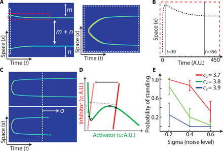
(A) (Left) Example of a traveling-to-standing transformation on a longer time scale. The pattern formation is indicated using the variables m and n that show equal spacing of standing branches on a periodic domain. (Right) Zoomed-in version of the activity in the white dashed box. (B) Time evolution of the activity in the red dashed space in (A), showing through the vertical lines the time taken to travel and stop versus the time taken to form the final pattern. (C) Example of deterministic (top) and stochastic (bottom) simulations, where noise (sigma) in the latter causes the standing branches to fall off. (D) Nullclines illustrating the falling off of the stable state to return to the original equilibrium (light red nullcline). (E) Average of 40 simulations with different levels of noise (sigma) and system threshold, which is controlled by the slope of the inhibitor nullcline (c2). A lower slope corresponds to a lower threshold and vice versa.
The previous results were in a deterministic setting with a manual trigger to create the wave. In a stochastic setting, however, a standing wave can end (Fig. 2, C and D), because a sufficiently large random perturbation may move the state away from the new equilibrium (Materials and Methods). Figure 2E shows that a low-threshold standing wave is more stable to stochastic perturbations. This occurs as the inhibitor gradient formed is stronger for lower threshold surroundings, which results in a larger threshold for the newly-formed equilibrium (fig. S1D).
Stable, confined protrusions observed in mutant cell types can be recreated using standing waves
During cell migration, amoeboid cells extend pseudopods, i.e., periodic protrusions of their cortex, to propel the cell forward. The extensions are controlled by waves of signaling molecules that organize actin polymerization near the membrane, creating protrusions that last around 60 s and cover 5 to 25% of the cell cortex (movie S2) (21). Mutant forms of Dictyostelium, such as those in which the tumor suppressor gene PTEN has been deleted (PTEN-null cells), are known to create elongated finger-like protrusions tipped by small regions of elevated signal transduction and cytoskeletal events (12, 27). Excitable waves cannot create these elongations, which require waves that neither spread nor die but persist at one particular region. Note that the coexistence of traveling waves and stable patterns does not depend on the cytoskeleton because latrunculin-treated cells, in which actin polymerization is inhibited, also display both phenomena (15). These patches are anomalous because, typically, responses of excitable systems oscillate, propagate, or extinguish.
Actin-inhibited amoeboid signaling waves (Materials and Methods) spin around the cell cortex (Fig. 3A), with the response at any given point lasting about 1 min. However, in the PTEN-null cells (Materials and Methods), a wave can linger at a portion of the cortex for over 4 min (Fig. 3B). These persistent patches, when coupled with the cytoskeleton, create the elongated finger-like protrusions (Fig. 3C and movie S3). These fingertips are also accompanied by accumulation of signaling markers (PHcrac shown in Fig. 3D). Often, the signal transduction and cytoskeletal events at the tips of the protrusions appear in the form of small rings of actin (Fig. 3E) that continually push on the cell boundary (28). The rings suggest that these finger-like protrusions were formed by waves that stopped quickly after being triggered but were not extinguished upon stopping. That is, the hole in the center of the rings suggests that the waves traveled some distance before the transformation occurred. As lowering threshold increases wave range (13), it was predicted that larger rings may appear after lowering the threshold of PTEN-null cells. This was confirmed by increasing the activity of PTEN-null cells using activated Ras. These cells displayed large, fluctuating rings at the edge of the cell [termed a “pancake cell” (12)] often lasting indefinitely, until the cell finally tore itself apart. Figure 3F shows the evolution of one of these large rings.
Fig. 3. Traveling and standing phenotypes in cell migration.
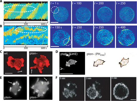
(A and B) Kymograph of PHcrac signaling marker for a latrunculin-treated wild-type (A) and PTEN-null (B) Dictyostelium cells. Images of the cells are shown on the right, with the white circle marked to follow activity at a small region. (C) Wild-type (wt) and PTEN-null cell morphology, with LimE-RFP. Scale bar, 5 μm. (D) PTEN-null example showing actin (left) and signaling (right) markers. Scale bar, 25 μm. (E) Actin dynamics in PTEN-null cells. Arrows indicate small actin rings. This panel is taken from (28) with permission. (F) F-actin wave pattern (GFP-LimE) phenotype induced by RasCQ62L expression in PTEN-null cells (scale bar, 5 μm) forming a pancake-type cell. This panel is taken from (12) with permission.
These experimental observations were recreated in simulations using the traveling-to-standing wave transformation. For a particular parameter regime, waves expanded and were extinguished to create typical protrusions (Fig. 4A and movie S4), as seen in wild-type amoeboid cells. In the standing parameter regime, however, activity persisted at one point in space lasting longer in time, creating elongated, finger-like extensions (Fig. 4B and movie S5). The cellular protrusions were modeled using a viscoelastic cell model in the level-set framework (Materials and Methods). The durations of protrusions that were similar in size (5 to 25% of the cortex) were quantified. The cells in Fig. 4B showed a significantly longer duration (Fig. 4C), although system turnaround time (ε) was not altered. A two-sample Kolmogorov-Smirnov test revealed that these two protrusive phenotypes belonged to different distributions (Materials and Methods). In one-dimensional simulations, it was difficult to appreciate the existence of small rings at the tips of protrusions. With a lowered threshold, however, the wave was expected to expand and create a larger standing wave that is, as previously demonstrated, more stable to stochastic perturbations. We simulated the formation of this “pancake” ring using a two-dimensional spatial simulation (Fig. 4D and movie S6). The wave initially traveled, stopped, and then evolved into a standing wave. Thereafter, the wave broke apart and rearranged to form a stable periodic pattern in space (t = 130 to 900 arbitrary time units). We conjecture that, in experiments, we do not see the periodic rearrangement within rings of the pancake cells for two reasons. First, the time scale for this to occur is over an order of magnitude larger. Second, the cell boundary has an organizing effect on the wave, which does not allow it to break up. In fig. S1E, we show through simulation, in which activator diffusion was spatially limited, that the standing wave organized as a stable ring at the boundary (movie S7).
Fig. 4. Simulations of the excitable system recreating experimentally observed wave and morphological phenotypes.
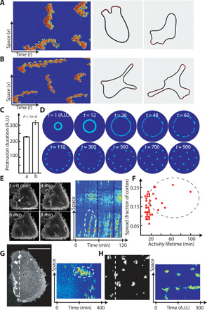
(A) (Left) Kymographs of normal amoeboid-type protrusions. The yellow dashed line indicates the traveling wave. (Right) Level-set simulations from the activity in (A). (B) (Left) Kymographs of a PTEN-null type protrusion, showing significantly longer thin fingers of activity. The yellow dashed line has much lower slope than that of (A), indicative of the slow velocity of a standing wave. (Right) Level-set simulations from the activity in (B), showing elongated protrusions. (C) Quantification of the duration of activity obtained through simulations from parameter sets of (A) and (B). Patches that covered between 5 and 25% of the domain size were quantified. P value obtained from t test for 180 protrusions. (D) Two-dimensional deterministic simulations manually triggering a wave at the center of the domain to study the time evolution of spatial activity. (E) Images and kymograph showing actin activity in transformed MCF-10A cells. Traveling waves are seen in the images (white arrow) and in the kymograph (dashed circle). Scale bar, 50 μm. (F) Quantification of wave durations seen in transformed MCF-10A cells (three cells). Each point corresponds to a protrusion. The points in the dashed circle indicate those that persisted longer than traveling waves typically do. (G) Images and corresponding kymographs showing PH-AKT activity in a transformed MCF-10A cell. Activity persists at a location (dashed circle) without spreading for over 100 min. Scale bar, 21 μm. (H) Similar standing activity from stochastic two-dimensional simulations.
Apart from Dictyostelium, we also looked at transformed cells where KRasG12V oncogenic mutation was introduced in MCF-10A epithelial cells (Materials and Methods). These cells similarly display spontaneous excitable waves on the cortex (Fig. 4E and movie S8). We quantified the two-dimensional wave activity through kymographs to study the spread and duration of these waves. On average, these waves lasted around 10 to 20 min at a particular point on the cortex (Fig. 4F). However, we observed numerous cases where the wave persisted for significantly longer durations (Fig. 4F, dashed circle), displaying the standing phenotype (Fig. 4G and movie S9). In all these cases, a membrane and cytosolic marker was used to rule out membrane undulations (fig. S2B). These cells demonstrate that both transient and persistent activity levels are observed experimentally. Two-dimensional spatially stochastic simulations showed remarkably similar wave phenotypes in which some waves traveled, while others lingered at one point for significantly longer durations (Fig. 4H and movie S10).
A phase diagram of cellular phenotypes reveals an all-encompassing protrusion template
Using a phase diagram of excitable system parameters, we characterized the regions where different protrusive phenotypes are observed (Fig. 5A). Two parameters were chosen, one controlling the negative feedback from the inhibitor and another controlling the time scale separation such that the lower left corner represented the lowest threshold and the upper left corner represented the highest. The red region denotes the set of parameters for which our initial stimulus was unable to elicit any response (subthreshold). The green region demarcates the region where a wave triggered, spread, and was extinguished at the critical wave-stopping threshold. The yellow region denotes the set of parameters for which the wave, at the critical threshold, transformed into a standing wave. To the left of the standing wave region is the parameter space for which the wave did not stop in the finite range of the cortex, and the two branches of the traveling wave spread until they met and annihilated.
Fig. 5. An all-encompassing protrusion template.
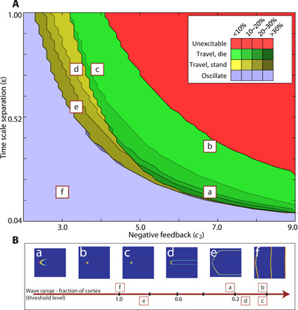
(A) Phase diagram showing different wave phenotypes through colors and wave ranges through shades. The letters correspond to the particular wave phenotypes. (B) Categorizing wave phenotype thresholds based on wave range, i.e., the fraction of simulation domain occupied by the wave. a, amoeboid; b and c, puncta/little waves; d, PTEN-null; e, pancake; f, oscillator.
As mentioned previously, a lower value of ε/Dv is necessary for standing wave formation. In this diagram, the diffusion coefficients were constant, but ε was varied. The standing wave zone (yellow) seems to thin out as ε is lowered. However, this occurs as lowering ε also causes waves to spread further (lower threshold), and owing to a finite domain size, the wave ends meet to annihilate, creating the oscillatory zone, before the stopping threshold is reached.
The threshold of wave types was also categorized based on wave range (Fig. 5B). These wave types were mapped onto different regions of the phase diagram depending on whether the waves covered 20 to 30% of the cortex (amoeboid, if not standing), 10 to 20% (PTEN-null like, if standing), or <10% (smaller puncta-type waves). Inside the standing wave zone, with a lower threshold than the simulated PTEN-null cells, was the pancake phenotype where the standing wave covered a larger portion of the cortex. To the left of the standing wave region were oscillator cells (13) that sustain waves that do not stop or stand but reappear in periodic cycles. The wave ranges are overlaid on the phase diagram using different color shades (Fig. 5A).
Information regarding the transitions between these phenotypes are also embedded within this phase diagram. Raising the threshold of amoeboid cells (“a” in Fig. 5A) resulted in smaller waves. However, these may be at different places of the phase diagram depending on which parameter was altered. For example, increasing the time scale separation moved the cell closer to the unexcitable zone (“b” in Fig. 5A). However, if negative feedback was concomitantly decreased, the cell moved to the cusp of the standing wave region (“c” and “d” in Fig. 5A). This change is consistent with the transition between wild-type cells and PTEN-null cells (“a” to “d”), in terms of the wave phenotype. Similarly, recruitment of PKBA (protein kinase B, Akt homolog) rapidly converted wild-type wave patterns to a punctate pattern (“a” to “c”) that generates numerous elongated protrusions (10). Experimentally, lowering phosphatidylinositol 4,5-bisphosphate [PI(4,5)P2] levels leads to a transformation from amoeboid to oscillator cells (13) by increasing positive feedback. In our diagram, a similar transformation that bypassed the standing wave region and enters the oscillator zone (“f” in Fig. 5A) was obtained by lowering negative feedback or by increasing positive feedback (fig. S2A). Inside the standing wave region, however, lowering threshold from PTEN-nulls led to larger, more stable, standing waves (“e” in Fig. 5A), as is seen experimentally in pancake cells (Fig. 3D) (12). The choice of negative feedback strength and time scale separation as parameters to explore the wave phenotypes was arbitrary. The same phenotypes and transitions were also obtained by varying positive feedback strength and negative feedback strength (fig. S2A). It was only necessary to choose parameters that have a direct effect on the threshold of the excitable system.
DISCUSSION
The existence of traveling and standing waves in excitable systems or in systems with limit cycle attractors has been well documented (25, 29). It has also been suggested that both patterns can coexist when diffusion coefficients are varied to realize a zero-wave speed scenario (9). However, it is unlikely to expect diffusion parameters to be altered in real time; hence, this transformation mechanism is difficult. Using the concept of wave stopping, we demonstrated how it is possible for a traveling wave to convert into a standing wave without altering the space-scale separation, i.e., the ratio of diffusion coefficients, directly.
The gradual conversion of a traveling wave to a standing wave without manually altering diffusion coefficients suggests a possible method of pattern generation. Most pattern formation theories suggest that patterns arise spontaneously because of an unstable spatially homogeneous state (6, 8), and that the resultant spots may then rearrange to form a final stable configuration (30, 31). We have shown that it is possible for a pattern to begin as a continuous traveling wave that ultimately slows down, stops, and transforms into discrete standing waves that then rearrange to form the resulting pattern (Fig. 4D). Note that Turing’s instability conditions (32) are not satisfied by our model (Materials and Methods); hence, in our system, pattern formation occurs owing to a combination of lateral inhibition and excitability (25).
In the context of cellular signaling dynamics, using this traveling-to-standing transformation, we were able to recreate situations in which activity on the cell cortex persisted at a point in space without spreading, in both Dictyostelium and mammalian mutant strains. While we do not claim to reproduce every phenotype completely, this study suggests a mechanism for both transient (traveling) and persistent (standing) activity on the cell cortex, a phenomenon that occurs often in cells, using an excitable system. The experiments provided here do not serve to rule out other possible mechanisms and only motivate the need for a model that can capture all wave phenotypes. An activator-inhibitor system approximates the underlying biological signaling network, and a more detailed model is necessary to completely recreate mutant phenotypes such as migratory or growth characteristics.
The phase diagram of Fig. 5A provides an interesting insight into how cell phenotypes are normally perceived. We have previously argued that these cellular protrusions lie on a continuum and are interchangeable by the overall state of the signaling and cytoskeletal system (10). Here, we have shown that this continuum has multiple dimensions and that an amoeboid cell may transition to different phenotypes depending on which way you go in transition diagram. One particular phenotype presents itself at multiple locations on the phase diagram, and so, the same phenotype may suggest transitions into different phenotypes based on where it started from. Simply put, one may not be able to predict a transition phenotype by merely studying a particular cell state. For example, cells in “b” and “c” in Fig. 5A have indistinguishable wave type. However, being at different locations on the transition diagram, increasing the activity of such a wave will create different phenotypes.
The phase diagram also provides numerous transition predictions. For example, it suggests that one can move from a pancake-type cell (12), which eventually fragments, to an active oscillator cell by lowering negative feedback (13). Depending on the strengths of the feedback loops altered in the overall excitable network architecture, it is theoretically possible to traverse through all these different phenotypes. In this study, we achieved this by manipulating time scale separation (or positive feedback) and negative feedback. In cells, this would translate to altering the threshold of the system by perturbing different nodes of the signal transduction system. For example, the amoeboid–to–PTEN-null transition (“a” to “d” in Fig. 5A) could be achieved by lowering negative feedback through one node while simultaneously increasing threshold through another. To know the exact correspondences of the feedback loops to biochemical species, a more detailed biochemical excitable model is needed. It is also worth noting that these standing waves only occur at the boundary of the cell and not in the interior. It is likely that surface contact alters cellular threshold and that the edge of the cell has a different state that allows the standing phenomenon to manifest. Experimentally, it would be interesting to alter the contact of the cells with the substrate to generate standing patterns inside the cell.
Many researchers have suggested the concept of bistability as a means to explain protrusive activity that do not propagate or die (15). That, in itself, cannot explain the wave propagation observed regularly on the cortex however. Although, one study illustrates how different patterns can arise as a refractory variable is introduced to a bistable model (33)—even that requires alterations to the model for different phenotypes. The traveling-to-standing wave bifurcation theory provides a seamless way to move within these phenotypes without having to alter the system drastically. A traveling wave may thus naturally persist for a longer duration at a particular point, allowing a cell to modulate its pseudopods.
MATERIALS AND METHODS
Simulation methods
The excitable system equations used to model the system were
The one-dimensional simulations of Figs. 1 and 2 assumed a periodic line of 600 points with dx = 0.05 in MATLAB (Natick, MA). For Fig. 5, a line of 1200 points was used. Diffusion was implemented using the central difference approximation. To add Gaussian white noise to the simulations, the SDE toolbox of MATLAB was used (34). Stability of standing waves was calculated by adding a particular noise variance and checked after a fixed time interval if the standing wave still persisted. Deterministic waves were triggered by increasing the initial activator concentration at a point in space. The exact level of noise was small enough to ensure that a new wave trigger did not initiate. The following excitable system parameters for the above equations were used: a1 = 0.167, a2 = 16.67, a3 = 167, a4 = 1.44, a5 = 1.47, c1 = 0.1, c2 = 4.2 (nonstanding), c2 = 3.9 (standing), epsilon = 0.52 (for Fig. 5, epsilon = 0.4), Du = 0.1, Dv = 1.
To determine whether Turing’s instability conditions hold (32), we note that the three required conditions are (a) fu + gv < 0, (b) fugv – fvgu > 0, (c) Dvfu + Dugv > 0, where the subscripts denote the partial derivatives. When “r = 0” and using the parameters listed above, conditions a (=−22.65) and b (=2.84) are satisfied for a stable equilibrium, but condition c (=−22.61) is not.
The one-dimensional simulations of Fig. 4 (A and B) were done using the package URDME (35), which implements the next subvolume method and allows a better approximation of system intrinsic noise. For this purpose, the parameters were scaled from concentrations to number of molecules using a multiplication factor of 18. Simulations were done on 314 points, with dx = 0.1. Nominal parameters for both simulations were as follows: a1 = 0.167, a2 = 16.67, a4 = 1.44, a5 = 1.47, c1 = 0.1, epsilon = 0.4, Du = 0.1 and Dv = 1. Parameters for Fig. 4A were as follows: a3 = 167, c2 = 2.1. Parameters for Fig. 4B were as follows: a3 = 300.6, c2 = 3.0. A sample size of 180 protrusions was used to conduct the Student’s t test, and the Kolmogorov-Smirnov test for protrusion durations.
The two-dimensional deterministic simulations of Fig. 4C were done using COMSOL Multiphysics 4.2a (Burlington, MA), using the same parameters as the MATLAB one-dimensional simulations, except that c2 = 4 and epsilon = 0.4 were used. Waves were triggered using a step input at the central point. The two-dimensional stochastic simulations of Fig. 4E were done using a two-dimensional version of URDME. The parameters were the same as in the one-dimensional URDME simulation, except that c2 = 2.8. A circular mesh of radius 8 units was created, where the maximum allowed distance between two nodes was 0.25.
The cell movement simulations were carried out using a viscoelastic cell membrane model (36), using the level-set toolbox of MATLAB (37), where the cell is modeled as a circle that is then subjected to stresses obtained from the activity from the wave simulations. This activity was applied to a viscoelastic cell, normal to the cell membrane. The total stresses included active stress from the waves, surface tension, and volume conservation. Details and parameter values for the level-set simulations can be found in (13).
Experimental methods
Dictyostelium
Cells and plasmids
The wild-type Dictyostelium discoideum cells of axenic AX2 strain were obtained from R. Kay laboratory (MRC Laboratory of Molecular Biology, UK). The pten− strain was generated in our laboratory from parent AX2 strain and was described previously (27). Both wild-type and gene knockout cell lines were cultured axenically in HL-5 medium at 22°C. Within 2 months of thawing the cells from the frozen stocks, the experiments were done. To visualize PIP3 dynamics, PHcrac was used as the biosensor. To visualize Ras activation, RBD (the Ras binding domain of Raf1) was used. LimEΔcoil was used to obtain newly polymerized F-actin dynamics. For exogenous gene expressions, Dictyostelium cells were transformed with PHcrac-mCherry, RBD-GFP (Ras-binding domain of mammalian Raf1, green fluorescent protein), LimEΔcoil-RFP (red fluorescent protein), or GFP-LimEΔcoil plasmids by electroporation and selected using either hygromycin B (50 μg/ml) or G418 (20 μg/ml), as per the antibiotic resistances of the vectors.
Cell preparation for microscopy
Growth phase cells were transferred to an eight-well Nunc Lab-Tek coverslip chamber and allowed to adhere for 10 min. Then, the HL-5 medium was replaced with 450 μl of development buffer (5 mM Na2HPO4, 5 mM KH2PO4, supplemented with 2 mM MgSO4 and 0.2 mM CaCl2). The cells were treated with 4 mM (final concentration) caffeine (Sigma-Aldrich; C0750) for 20 min to visualize more waves, as reported previously (38). To inhibit cytoskeletal input in signaling dynamics, the actin polymerization inhibitor latrunculin A (Enzo Life Sciences; BML-T119) was added to cells at a final concentration of 5 μM and then cells were incubated for around 25 min.
Confocal microscopy and image processing
The time-lapse confocal images were acquired using a Zeiss LSM780 single-point laser scanning confocal microscope (Zeiss Axio Observer with 780-Quasar; 34-channel spectral, high-sensitivity gallium arsenide phosphide detectors), illuminated by 488 nm (argon laser) for GFP or by 561 nm (solid-state laser) for mCherry and RFP. All experiments were performed in 40×/1.30 Plan-Neofluar oil objective. The images were processed using Fiji/ImageJ [National Institutes of Health (NIH)]. Kymographs were generated by a custom-written MATLAB script. The LimE-mRFP– and PHcrac-YFP (yellow fluorescent protein)–expressing pten− cells in Fig. 3D were imaged in every 4-s interval. The LimE is shown in “Grays” and the PHcrac is shown in “Fire Invert LUT” of Fiji/ImageJ (NIH). The majority of background cytosolic signal was subtracted in PHcrac channel for clarity.
MCF-10A
Cells
MCF-10A cell (acquired from Iijima laboratory of Johns Hopkins University) and Kras (G12V) MCF-10A cell (generated by viral transfection) were grown at 37°C in 5% CO2 using Dulbecco’s modified Eagle’s medium/F-12 medium (Gibco, #10565042) supplemented with 5% horse serum (Gibco, #26050088), epidermal growth factor (EGF) (20 ng/ml) (Sigma-Aldrich, #E9644), cholera toxin (100 ng/ml) (Sigma-Aldrich, #C-8052), hydrocortisone (0.5 mg/ml) (Sigma-Aldrich, #H-0888), and insulin (10 μg/ml) (Sigma-Aldrich, #I-1882).
Stable Kras (G12V) MCF-10A cell line was selected and maintained in culture medium containing puromycin (2 μg/ml) (Thermo Fisher Scientific, #A1113803) after virus transfection. LYN-FRB, FKBP-INP54P, PH-AKT, and LIFEACT stable cell lines were sorted by fluorescence tags after virus transfection.
Cells were transferred to 35-mm glass-bottom dishes (MatTek, #P35G-0.170-14-C) or chambered coverglass (Lab-Tek, #155409PK) and allowed to attach overnight at 37°C in 5% CO2 before imaging. Cells were kept in phenol red–free culture medium at 37°C in 5% CO2 during microscope imaging.
Plasmids
Constructs of CFP-Lyn-FRB and mCherry-FKBP-INP54P were obtained from Inoue laboratory (Johns Hopkins University). GFP/RFP-PH-AKT, RFP-LifeAct, pFUW2, pMDL, pRSV, and pCMV were obtained from Desiderio laboratory (Johns Hopkins University). pBABE-KrasG12V (#9052), pUMVC (#8449), and pCMV-VSV-G (#8454) constructs were obtained from Addgene. Lyn-FRB, FKBP-INP54P, PH-AKT, and LifeAct were subcloned into lentiviral expression plasmid pFUW2.
Drugs
The EGF stock solution was prepared by dissolving EGF (Sigma-Aldrich, #E9644) in 10 mM acetic acid to a final concentration of 1 mg/ml. Insulin (Sigma-Aldrich, #I-1882) was resuspended at 10 mg/ml in sterile ddH2O containing 1% glacial acetic acid. Hydrocortisone (Sigma-Aldrich, #H-0888) was resuspended at 1 mg/ml in 200 proof ethanol. Cholera toxin (Sigma-Aldrich, #C-8052) was resuspended at 1 mg/ml in sterile ddH2O and stored at 4°C. All drug stocks except cholera toxin were stored at −20°C.
Virus generation
Twenty-five milliliters of 293T cells was seeded at 6 × 10⁵/ml to 15-cm cell culture dishes on day 1. Conventional calcium phosphate transfection was performed on day 2 to deliver expressing and packaging plasmids into 293T cells. pFUW2 (20 μg), pMDL (9.375 μg), pRSV (9.375 μg), pCMV plasmids (9.375 μg) (or 10 μg of pBABE, 9 μg of pUMVC, 1 μg of pCMV-VSV-G), CaCl2 (250 μl), and ddH2O in a total volume of 2.5 ml were mixed with 2.5 ml of 2× Hepes (pH 7.05) and incubated for 5 min. The transfection mix was added to the plated cells and shaken gently. Medium was changed after 4 to 6 hours. For virus collection, the medium from infected cells was collected on day 5 and spun at 1000 rpm for 3 min to remove the debris and filtered through 0.45-μm filter followed by ultracentrifugation at 25,000 rpm for 90 min at 4°C in a Beckman ultracentrifuge. The supernatant was discarded and the pellet was dissolved in 70 μl of phosphate-buffered saline overnight at 4°C to obtain concentrated virus, which was stored as 25-μl aliquots at −80°C.
Microscopy
Confocal microscopy was carried out on Zeiss Axio Observer inverted microscope with either LSM780-Quasar (34-channel spectral, high-sensitivity gallium arsenide phosphide detectors, GaAsP) or LSM800 confocal module controlled by the Zen software. All live cell imaging was carried out in a temperature/humidity/CO2-regulated chamber. The signaling/cytoskeletal waves on the cell ventral surface were obtained by capturing the confocal slice of the very bottom of the cell.
Supplementary Material
Acknowledgments
Funding: This work was supported, in part, by DARPA under contract number HR0011-16-C-0139 (P.A.I.), NIH/NIGMS R35 GM11817735 (P.N.D.), and AFOSR MURI FA95501610052 (P.N.D.). Author contributions: S.B. performed all theoretical analysis and simulations; T.B., Y.M., and H.Z. carried out the experimental imaging under the supervision of P.N.D. P.A.I. directed the study. S.B. and P.A.I. wrote the paper, which was approved by all authors. Competing interests: The authors declare that they have no competing interests. Data and materials availability: All data needed to evaluate the conclusions in the paper are present in the paper and/or the Supplementary Materials. Simulations files are available by request from P.A.I. Experimental materials are available by request from P.N.D. Additional data related to this paper may be requested from the authors.
SUPPLEMENTARY MATERIALS
Supplementary material for this article is available at http://advances.sciencemag.org/cgi/content/full/6/32/eaay7682/DC1
REFERENCES AND NOTES
- 1.Pertsov A. M., Davidenko J. M., Salomonsz R., Baxter W. T., Jalife J., Spiral waves of excitation underlie reentrant activity in isolated cardiac muscle. Circ. Res. 72, 631–650 (1993). [DOI] [PubMed] [Google Scholar]
- 2.Devreotes P. N., Bhattacharya S., Edwards M., Iglesias P. A., Lampert T., Miao Y., Excitable signal transduction networks in directed cell migration. Annu. Rev. Cell Dev. Biol. 33, 103–125 (2017). [DOI] [PMC free article] [PubMed] [Google Scholar]
- 3.Tyson J. J., Keener J. P., Singular perturbation theory of traveling waves in excitable media (a review). Physica D 32, 327–361 (1988). [Google Scholar]
- 4.Bhattacharya S., Iglesias P. A., Controlling excitable wave behaviors through the tuning of three parameters. Biol. Cybern. 113, 61–70 (2019). [DOI] [PubMed] [Google Scholar]
- 5.Zhabotinsky A. M., Eager M. D., Epstein I. R., Refraction and reflection of chemical waves. Phys. Rev. Lett. 71, 1526–1529 (1993). [DOI] [PubMed] [Google Scholar]
- 6.Gierer A., Meinhardt H., A theory of biological pattern formation. Kybernetik 12, 30–39 (1972). [DOI] [PubMed] [Google Scholar]
- 7.H. Meinhardt, The Algorithmic Beauty of Sea Shells (Springer Science & Business Media, 2009). [Google Scholar]
- 8.Turing A. M., The chemical basis of morphogenesis. Philos. Trans. R. Soc. Lond. B Biol. Sci. 237, 37–72 (1952). [DOI] [PMC free article] [PubMed] [Google Scholar]
- 9.Dockery J., Keener J., Diffusive effects on dispersion in excitable media. SIAM J. Appl. Math. 49, 539–566 (1989). [Google Scholar]
- 10.Miao Y., Bhattacharya S., Banerjee T., Abubaker-Sharif B., Long Y., Inoue T., Iglesias P. A., Devreotes P. N., Wave patterns organize cellular protrusions and control cortical dynamics. Mol. Syst. Biol. 15, e8585 (2019). [DOI] [PMC free article] [PubMed] [Google Scholar]
- 11.Mori Y., Jilkine A., Edelstein-Keshet L., Wave-pinning and cell polarity from a bistable reaction-diffusion system. Biophys. J. 94, 3684–3697 (2008). [DOI] [PMC free article] [PubMed] [Google Scholar]
- 12.Edwards M., Cai H., Abubaker-Sharif B., Long Y., Lampert T. J., Devreotes P. N., Insight from the maximal activation of the signal transduction excitable network in Dictyostelium discoideum. Proc. Natl. Acad. Sci. U.S.A. 115, E3722–E3730 (2018). [DOI] [PMC free article] [PubMed] [Google Scholar]
- 13.Miao Y., Bhattacharya S., Edwards M., Cai H., Inoue T., Iglesias P. A., Devreotes P. N., Altering the threshold of an excitable signal transduction network changes cell migratory modes. Nat. Cell Biol. 19, 329–340 (2017). [DOI] [PMC free article] [PubMed] [Google Scholar]
- 14.Meinhardt H., Orientation of chemotactic cells and growth cones: Models and mechanisms. J. Cell Sci. 112, 2867–2874 (1999). [DOI] [PubMed] [Google Scholar]
- 15.Matsuoka S., Ueda M., Mutual inhibition between PTEN and PIP3 generates bistability for polarity in motile cells. Nat. Commun. 9, 4481 (2018). [DOI] [PMC free article] [PubMed] [Google Scholar]
- 16.S. Bhattacharya, D. Biswas, G. A. Enciso, P. A. Iglesias, Control of chemotaxis through absolute concentration robustness, in 2018 IEEE Conference on Decision and Control (CDC) (IEEE, 2018), pp. 4360–4365. [Google Scholar]
- 17.FitzHugh R., Impulses and physiological states in theoretical models of nerve membrane. Biophys. J. 1, 445–466 (1961). [DOI] [PMC free article] [PubMed] [Google Scholar]
- 18.Nagumo J., Arimoto S., Yoshizawa S., An active pulse transmission line simulating nerve axon. Proc. IRE 50, 2061–2070 (1962). [Google Scholar]
- 19.Bhattacharya S., Iglesias P. A., The threshold of an excitable system serves as a control mechanism for noise filtering during chemotaxis. PLOS ONE 17, e0201283 (2018). [DOI] [PMC free article] [PubMed] [Google Scholar]
- 20.Shi C., Huang C.-H., Devreotes P. N., Iglesias P. A., Interaction of motility, directional sensing, and polarity modules recreates the behaviors of chemotaxing cells. PLOS Comput. Biol. 9, e1003122 (2013). [DOI] [PMC free article] [PubMed] [Google Scholar]
- 21.Huang C.-H., Tang M., Shi C., Iglesias P. A., Devreotes P. N., An excitable signal integrator couples to an idling cytoskeletal oscillator to drive cell migration. Nat. Cell Biol. 15, 1307–1316 (2013). [DOI] [PMC free article] [PubMed] [Google Scholar]
- 22.Tang M., Wang M., Shi C., Iglesias P. A., Devreotes P. N., Huang C.-H., Evolutionarily conserved coupling of adaptive and excitable networks mediates eukaryotic chemotaxis. Nat. Commun. 5, 5175 (2014). [DOI] [PMC free article] [PubMed] [Google Scholar]
- 23.Li X., Edwards M., Swaney K. F., Singh N., Bhattacharya S., Borleis J., Long Y., Iglesias P. A., Chen J., Devreotes P. N., Mutually inhibitory Ras-PI(3,4)P2 feedback loops mediate cell migration. Proc. Natl. Acad. Sci. U.S.A. 115, E9125–E9134 (2018). [DOI] [PMC free article] [PubMed] [Google Scholar]
- 24.P. C. Fife, Non-Equilibrium Dynamics in Chemical Systems (Springer, 1984), pp. 76–88. [Google Scholar]
- 25.Ermentrout G., Hastings S., Troy W., Large amplitude stationary waves in an excitable lateral-inhibitory medium. SIAM J. Appl. Math. 44, 1133–1149 (1984). [Google Scholar]
- 26.Iglesias P. A., Devreotes P. N., Navigating through models of chemotaxis. Curr. Opin. Cell Biol. 20, 35–40 (2008). [DOI] [PubMed] [Google Scholar]
- 27.Iijima M., Devreotes P., Tumor suppressor PTEN mediates sensing of chemoattractant gradients. Cell 109, 599–610 (2002). [DOI] [PubMed] [Google Scholar]
- 28.Lampert T. J., Kamprad N., Edwards M., Borleis J., Watson A. J., Tarantola M., Devreotes P. N., Shear force-based genetic screen reveals negative regulators of cell adhesion and protrusive activity. Proc. Natl. Acad. Sci. U.S.A. 114, E7727–E7736 (2017). [DOI] [PMC free article] [PubMed] [Google Scholar]
- 29.Kohsokabe T., Kaneko K., Boundary-induced pattern formation from uniform temporal oscillation. Chaos 28, 045110 (2018). [DOI] [PubMed] [Google Scholar]
- 30.Meinhardt H., Pattern formation in biology: A comparison of models and experiments. Rep. Prog. Phys. 55, 797 (1992). [Google Scholar]
- 31.Kondo S., Miura T., Reaction-diffusion model as a framework for understanding biological pattern formation. Science 329, 1616–1620 (2010). [DOI] [PubMed] [Google Scholar]
- 32.T. Leppänen, Current Topics in Physics: In Honor of Sir Roger J Elliott (World Scientific, 2005), pp. 199–227.
- 33.Holmes W. R., Carlsson A. E., Edelstein-Keshet L., Regimes of wave type patterning driven by refractory actin feedback: Transition from static polarization to dynamic wave behaviour. Phys. Biol. 9, 046005 (2012). [DOI] [PMC free article] [PubMed] [Google Scholar]
- 34.U. Picchini, SDE toolbox: Simulation and estimation of stochastic differential equations with Matlab (2007); http://sdetoolbox.sourceforge.net.
- 35.Drawert B., Engblom S., Hellander A., URDME: A modular framework for stochastic simulation of reaction-transport processes in complex geometries. BMC Syst. Biol. 6, 76 (2012). [DOI] [PMC free article] [PubMed] [Google Scholar]
- 36.Yang L., Effler J., Kutscher B. L., Sullivan S. E., Robinson D. N., Iglesias P. A., Modeling cellular deformations using the level set formalism. BMC Syst. Biol. 2, 68 (2008). [DOI] [PMC free article] [PubMed] [Google Scholar]
- 37.Mitchell I. M., The flexible, extensible and efficient toolbox of level set methods. J. Sci. Comput. 35, 300–329 (2008). [Google Scholar]
- 38.Arai Y., Shibata T., Matsuoka S., Sato M. J., Yanagida T., Ueda M., Self-organization of the phosphatidylinositol lipids signaling system for random cell migration. Proc. Natl. Acad. Sci. U.S.A. 107, 12399–12404 (2010). [DOI] [PMC free article] [PubMed] [Google Scholar]
Associated Data
This section collects any data citations, data availability statements, or supplementary materials included in this article.
Supplementary Materials
Supplementary material for this article is available at http://advances.sciencemag.org/cgi/content/full/6/32/eaay7682/DC1