Abstract
The development of automated tools for brain morphometric analysis in infants has lagged significantly behind analogous tools for adults. This gap reflects the greater challenges in this domain due to: 1) a smaller-scaled region of interest, 2) increased motion corruption, 3) regional changes in geometry due to heterochronous growth, and 4) regional variations in contrast properties corresponding to ongoing myelination and other maturation processes. Nevertheless, there is a great need for automated image-processing tools to quantify differences between infant groups and other individuals, because aberrant cortical morphologic measurements (including volume, thickness, surface area, and curvature) have been associated with neuropsychiatric, neurologic, and developmental disorders in children. In this paper we present an automated segmentation and surface extraction pipeline designed to accommodate clinical MRI studies of infant brains in a population 0-2 year-olds. The algorithm relies on a single channel of T1-weighted MR images to achieve automated segmentation of cortical and subcortical brain areas, producing volumes of subcortical structures and surface models of the cerebral cortex. We evaluated the algorithm both qualitatively and quantitatively using manually labeled datasets, relevant comparator software solutions cited in the literature, and expert evaluations. The computational tools and atlases described in this paper will be distributed to the research community as part of the FreeSurfer image analysis package.
Keywords: Segmentation, Infant, FreeSurfer, MRI, Brain surface
1. Introduction
Automated brain image segmentation of postnatal infant scans has received increased attention in recent years, given the unmet needs of clinical and neuroscience applications (Išgum et al., 2015; Makropoulos et al., 2017a; Alexander et al., 2017). The age range we address in this paper is the first 2 postnatal years, during which myelination as well as brain size and shape are most rapidly changing and begin to plateau. We have chosen the term “infant” as a default descriptor, loosely referring to children during the earliest period of life.
FreeSurfer (http://surfer.nmr.mgh.harvard.edu/), a widely used processing suite for brain MRIs, has evolved for nearly 20 years. The algorithms in FreeSurfer were originally designed for and extensively tested on adult datasets (Dale et al., 1999; Dale and Sereno, 1993a; Fischl and Dale, 2000a; Fischl et al., 1999a, 1999b, 2001, 2002, 2004a, 2004b; Han et al., 2006; Jovicich et al., 2005; Segonne et al., 2004a), but their use in children as young as 4.5 years has also met with success (Ghosh et al., 2010). Further extending the present capabilities to encompass the full postnatal period would be highly beneficial. Not only have alterations in cortical morphologic measurements (including volume, thickness, surface area, and curvature) been associated with neuropsychiatric, neurologic, and developmental disorders in children (Ecker et al., 2009; Li, 2016; Pacheco et al., 2015; Sierra et al., 2014), but a greater prevalence of those surviving perinatal injuries is now apparent (Johnson and Marlow, 2011; Bellinger et al., 2003; Limperopoulos et al., 2002; Rysavy et al., 2015). Such infants grow to adulthood, exhibiting multiple sequelae that are poorly understood. This trend intensifies the need for a unified image-processing approach applicable to a broad range of ages, as opposed to single time-point scenarios. It is important to note that a unified method does not imply a singular procedure for all participating ages but rather the harnessing of tools that automatically adapt to various input images, while yielding comparable quantitative measures as outcomes.
Most existing solutions focusing on pediatric image analysis are heavily specialized with respect to specific age ranges and imaging modalities and differ vastly in terms of resultant segmentation information. Thus, direct comparisons and evaluations remain a challenge. Strict intensity-based segmentation of these images is a difficult task, due to contrast intensity reversal in younger (vs. older) subjects (related to myelination), the relative excess of motion typically found in scans from this population, and the diminutive overall anatomy relative to voxel resolution. For these reasons, a majority of currently available solutions utilize prior information to varying degrees, which we summarize below.
1.1. Atlases
Many automated segmentation tools rely on the creation and usage of training datasets. These encode information on the population of interest and are often inseparable from the segmentation tools that they support. The information stored may refer to anatomic regions of interest (ROIs), average intensity, image intensity distributions, and/or or tissue probability maps. Given the multitude of challenges in infant populations, few methods rely exclusively on intensity information from input images without guidance from such sources (http://brainvis.wustl.edu; Gui et al., 2012).
Training datasets often include manually labeled regions related to the anatomy studied. The information embedded in individuals of the set could be summarized into a single probabilistic atlas (parametric approaches) or used individually, later combining the results (multi-atlas segmentation, non-parametric approaches). In this paper, the term atlas refers to one member of the training dataset (MRI volume and corresponding manual labels), whereas probabilistic atlas entails an average volume and corresponding label probabilities. Of note, some probabilistic atlases may only include intensity information, only label probabilities (e.g., SPM (Penny et al., 2006)) or both (e.g., FreeSurfer (http://surfer.nmr.mgh.har)).
It is challenging to directly compare the nature and the performance of existing infant training datasets with respect to segmentation, considering the wide variability of age ranges represented, modality of images they rely upon, the number of subjects they contain or summarize, their representation, the nature of the training subjects (for example, prematurely born or full-term newborn infants), the origin of the ROI labels (manual annotation directly drawn on the training set subjects or labels projected onto the training data sets) as well as the type of information that they contain, whether it is (sub)cortical labels, average intensity values, tissue probability maps, white matter pathways, or fractional anisotropy (FA) maps. Generally, they are characterized jointly by the tools using them, which in our case are full brain segmentation solutions.
Training datasets published in the literature to date include the following: (i) UNC: 0-1-2 (Shi et al., 2011) (N = 95, M = 90 labels drawn from Automated Anatomical Labeling (AAL) map (Tzourio-Mazoyer et al., 2002), K = 1 atlas); (ii) the UNC cortical (Li, 2015) (N = 35, K = 7 [time points]); (iii) the Imperial Pediatric Atlas (Gousias et al., 2008) (N = 33, M = 83, K = 33; ROIs derived from 30 manually labeled adults); (iv) the Imperial Neonatal Atlas (Kuklisova-Murgasova et al., 2011) (N = 153, M = 6, K = 1; average intensity and tissue probability maps and labels extracted from three neonatal reference subjects); (v) the Imperial Spatio-Temporal Atlas (Serag et al., 2012) (N = 204, M = 6, K = 17; relying upon Imperial Neonatal Atlas); (vi) the Imperial ALBERTs (Gousias et al., 2012) (N = 20, M = 50, K = 20); (vii) the USC (Sanchez et al., 2012) (N = 105 + 49, K = 13); (viii) the INSERM atlas (Dehaene-Lambertz et al., 2002) (N = 20, K = 1; average T2-weighted intensity); (ix) Akiyama atlas (http://ilabs.washington.e) (N = 60, M = 116; mapped AAL labels; K = 1); (x) Singapore (http://www.bioeng.nus.edu) (N = 112 and 32, K = 2; average intensity, FA, and DTI color map); (xi) the JHU: neonate atlas (Oishi et al., 2011) (K = 1; labeled from a manually annotated single subject; M = 122 structures based on diffusion-based imaging and fiber pathways); (xii) M-CRIB (Alexander et al., 2017) (N = 10, M = 100; cortical and subcortical labels matching the Desikan-Killiany parcellation (Desikan et al., 2006)); and (xiii) our Infant FreeSurfer atlases (de Macedo Rodrigues et al., 2015) (N = 26, M = 32 + 14, K = 26).
Considering the availability of clinical data and clinical interest in prematurity, many neonatal training datasets are built on images of prematurely born subjects obtained at term-equivalent ages (Gousias et al., 2008, 2012; Kuklisova-Murgasova et al., 2011; Serag et al., 2012). This is important to note, because reliance on applications rooted in prior information may introduce bias. For a more comprehensive summary of the above information, see Appendix Table 1.
1.2. Segmentation tools
A majority of existing postnatal infant segmentation tools are restricted to analysis of newborns (http://brainvis.wustl.edu; Gui et al., 2012; Gousias et al., 2013; Prastawa et al., 2005; Wang et al., 2015; Wang, 2013; Wang et al., 2011b; Beare et al., 2016; Makropoulos et al., 2014; Weisenfeld and Warfield, 2009), often focusing on or explicitly accommodating preterm subjects (http://brainvis.wustl.edu; Gui et al., 2012; Gousias et al., 2013; Makropoulos et al., 2014). Other algorithmic solutions have been designed for discrete age points within the first postnatal year (0, 3, 6, 9, 12 months) (Wang et al., 2015) or for 2 year-olds (Gousias et al., 2008; Dai, n.d.). Although primarily introduced to evaluate single-time point acquisitions, some require or accommodate access to longitudinal intra-subject imaging series, thus facilitating segmentation of more challenging younger-aged subjects (Wang, 2013, 2011b).
Given the relatively higher contrast between cerebral tissues in the immature brain (Dubois et al., 2008), most tools currently used at the newborn stage rely on T2-weighted MR input images, either in part or entirely. Some require only a single modality (Gousias et al., 2008, 2013; Beare et al., 2016; Makropoulos et al., 2014), whereas others use multiple channels (Gui et al., 2012; Prastawa et al., 2005; Wang, 2013, 2011b, 2015; Weisenfeld and Warfield, 2009). We are aware of only one pipeline that accommodates a single T1-weighted volume for segmentation of newborns or 2 year-olds (Gousias et al., 2008, 2013). In our view, relying on T1-weighted MPRAGE scans is preferable, as they are the only volumetric sequence acquired at all age groups in most clinical protocols. Indeed, these can be obtained at 1-mm isotropic resolution during a reasonable scan time, due to the ability to accelerate in two planes. In contrast, volumetric T2-weighted images are not used in infants due to poor contrast. Typically, only 2D T2-weighted MRI sequences are acquired with high in-plane resolution, but at 2.5- to 4-mm thickness, which is insufficient to resolve cortical folds.
The labels produced by current segmentation solutions also vary to a large extent. Most pipelines are aimed at tissue segmentation, i.e. labeling cortical gray matter [GM] or white matter [WM], often reflecting myelinated and unmyelinated areas, and cerebrospinal fluid [CSF]) (http://brainvis.wustl.edu; Gui et al., 2012; Prastawa et al., 2005; Wang et al., 2015; Wang, 2013; Wang et al., 2011b; Beare et al., 2016; Weisenfeld and Warfield, 2009). Likewise, brainstem and cerebellum (Gui et al., 2012; Beare et al., 2016) are often labeled. Various sets of cortical and subcortical regions, including those matching the AAL (Tzourio-Mazoyer et al., 2002) atlas description (Shi et al., 2011; http://ilabs.washington.e; Wang, 2013; Wang et al., 2011b), regions of interests defined by (Tzourio-Mazoyer et al., 2002; Hammers et al., 2003) in in (Gousias et al., 2008, 2012), and cortical and subcortical information matching FreeSurfer labels (Alexander et al., 2017) have also been used, and myelinated vs unmyelinated WM labels recovered (Weisenfeld and Warfield, 2009).
In some segmentation frameworks, age-specific infant atlases (for subjects ≤2 years of age) are used as guidance (Gousias et al., 2008, 2013; Prastawa et al., 2005; Wang et al., 2015; Beare et al., 2016; Makropoulos et al., 2014; Weisenfeld and Warfield, 2009); but in others, segmentation labels are extrapolated from adult-based atlases. For example, the AAL atlas, derived from the anatomical parcellation of a spatially normalized single adult subject, is often invoked. In (Wang, 2013, 2011b), high-resolution T1 volumes are transferred from older pediatric subjects (2 year-olds) to segment newborn acquisitions. Alternatively, in the Imperial:Pediatric tool (Gousias et al., 2008), a set of manually labeled adult acquisitions are used as prior information (30 adults, 83 ROIs). In one application (Wang et al., 2015), the authors use a semi-automatically populated infant population (<1 year of age) for this purpose.
A more comprehensive summary of above information is found in Appendix Table 2.
1.3. Surface extraction
Currently, only a few infant image-processing packages generate cortical surface models. Some authors (Dubois et al., 2008) have segmented and reconstructed surfaces in 3D using image post-processing tools adapted from sequences developed for brains of adults (Mangin et al., 2004) and fetuses (Cachia et al., 2003). Specifically, NEOCIVET (Kim, 2015) was introduced as a modification of the adult image-processing pipeline CIVET (Kim et al., 2005; MacDonald et al., 2000) and made applicable to preterm data. A surface-based probabilistic atlas of human cortical structure from 12 healthy term born infants has been created (Hill et al., 2010), and a 4D high-definition cortical surface atlas of infants (Li, 2015) has been computed using a topology-preserving deformable surface method (Li et al., 2012, 2014b). Two datasets released by The Developing Human Connectomee Project (dHCP) (Developing Human Connectome) have involved minimal pipeline processing (Bastiani et al., 2019), relying on a set of tools (i.e. a deformable model (Schuh, 2017), a spherical projection (Elad et al., 2005), and the FreeSurfer white matter inflation tool (Fischl et al., 1999c)) for approximating surfaces to independently computed cortical GM and WM segmentation labels (Makropoulos et al., 2017b).
1.4. Contribution
Our proposed tool is an automated segmentation and surface extraction pipeline designed to accommodate clinical infant T1-weighted brain MRIs from a population of 0–2 year-olds. The algorithm only requires a single channel MRI volume and produces automated segmentations of cortical and subcortical areas of the brain, including volumes and surfaces. The segmentation procedure adapts to the detected (or developmental) age of input data, allowing use of subsets within a manually labeled database that are optimal for each age range. This results in a unified procedure that can be applied across the full age range of interest, without sacrificing accuracy. Although the current pipeline is designed for T1-weighted images, equipped with appropriate training datasets, it would be straightforward to extend it to accommodate T2-weighted image volumes or multi-channel datasets.
2. Materials and methods
Our pipeline is a multi-stage process closely following the adult-oriented reconstruction pipeline of FreeSurfer (Dale et al., 1999; Fischl et al., 1999d; Fischl, 2012). The outputs generated are consistent with its reconstruction stream, facilitating consistency in future longitudinal studies. Fig. 1 demonstrates the major image processing steps in the standard FreeSurfer reconall pipeline, where red boxes indicate the ones that are different and were specifically introduced for an infant population. In this section, we focus on these particular algorithmic components.
Fig. 1.

Major image processing steps in the standard FreeSurfer reconall pipeline. Red boxes indicate the ones that are different and were specifically modified in the case of the infant-specific tools.
2.1. Skullstripping
Extraction of brain tissue and exclusion of the skull and extra-meningeal tissue from input images are crucial early steps of any neuroimaging pipeline. Infant MRIs show large inter-subject variability, due to rapid and heterogeneous brain development. There is also a less conspicuous gap between the cerebral cortex and the skull, and lower contrast is encountered among assorted cerebral tissues. Many automated skullstrippers were primarily designed for adults (Smith, 2002; Shattuck and Leahy, 2002; D Rex Woods et al., 2004; K Leung Modatet al., 2011; Segonne et al., 2004b; Doshi et al., 2013) and underperform on newborn datasets. Furthermore, the existing and publically available tools specifically introduced for infants (Dai, n.d.; Shi et al., 2012; Mahapatra, 2012; Ou et al., 2015) do not consistently accommodate our T1-weighted clinical datasets.
We used our novel double-consensus skullstripping approach to identify brain regions (Ou et al., 2018), applying a modified version of a tool developed by Doshi et al. (2013). In this framework, we first from a consensus by a multi-atlas approach, where the result is an initial brain mask for the subject. With the initial brain mask serving as a reference, we select a subset of candidate masks from a candidate pool containing both candidate masks generated from skull-strippers at various parameter settings, and candidate masks transferred into the subject space by atlas-to-subject registrations. The selected candidate masks then form a second consensus to get the final results. In our design, we used publicly-available pediatric atlases instead of the adult atlas of (K Leung Modatet al., 2011; Doshi et al., 2013). In particular, twelve were constructed from the NIH-PD database (Fonov et al., 2011) and three additional ones were randomly selected samples from secondary pediatric training datasets (Gousias et al., 2008). Their diversity in terms of ages, imaging institutions, scanners, field strengths, and pulse sequences helped us in increasing robustness. We also relied on multiple skullstrippers (BET (Smith, 2002), BSE (Shattuck et al., 2001), 3dSkullStrip [AFNI] (https://afni.nimh.nih.gov), HWA (Segonne et al., 2004b), and ROBEX (JE et al., 2011)). For transforming brain masks from atlas spaces into the subject space, we used the publicly-available Deformable Registration via Attribute Matching and Mutual-Saliency Weighting (DRAMMS) tool (Ou et al., 2011) and for fusing multiple atlas-implied brain masks into one mask, we used the publicly-available STAPLE label fusion tool (Warfield et al., 2004) due to their demonstrated accuracy and popularity in skull stripping problems (Doshi et al., 2013; Shi et al., 2012). Importantly, our method selects parameters that are optimal for each subject (not the entire dataset!). The flowchart of our skull-stripping pipeline is shown in Supplementary Figure 1 and its full description is provided elsewhere (Ou et al., 2018).
2.2. Volumetric segmentation
We designed a multi-atlas label fusion segmentation framework (Iglesias and Sabuncu, 2015) where ground-truth information from our labeled training data could be used for the segmentation of new infant brain images. Our solution was inspired by (Iglesias et al., 2012) and (Iglesias et al., 2013), which is in turn an MRI-contrast adaptive version of the Bayesian multi-atlas algorithm proposed by Sabuncu et al. (2010). The method relies on a generative model of imaging data, which is represented in Fig. 2, and uses Bayesian inference to compute the most likely segmentation. In short, this method assumes that a number of atlases have been registered to the scan to segment, provided N different candidate label maps Ln,n = 1,…,N. A discrete membership field M(x) ∈ {1,…,N}, which is assumed to be a sample of a Markov Random Field parameterized by β (and thus smooth), subsequently indexes from which atlas the segmentation of the target scan L has been generated (Eq (1)). Given the membership at a voxel x, the segmentation L(x) is assumed to be a sample of a logOdds model defined on the distance transform of LM(x) (Eq (2)). This segmentation is generated independently at each voxel. Given the segmentation L of the test scan, its intensities I are assumed to be independent samples of Gaussian distributions parameterized by label-dependent means and variances (μL, ), further corrupted by a multiplicative bias field. This bias field is assumed to be non-negative and smooth. Therefore, we model it as the exponential of a linear combinaion of smooth basis functions ψp (Eq (4)).
Fig. 2.

The proposed graphical model for our multi-atlas label fusion tool. Plates indicate replication, shaded variables are observed.
| (1) |
| (2) |
| (3) |
| (4) |
According to this model, segmentation can be cast as a Bayesian inference problem: given the image I and registered atlas segmentations Ln, the goal is to find the most likely segmentation L. Ideally, one would directly maximize p(L|Ln, I) but this leads to an intractable integral over the model parameters (θ = means, variances, and bias field coefficients). Instead, we make the standard approximation that the posterior distribution of these parameters is heavily peaked around their mode . Then, we can first compute this mode (“point estimates”) as , and subsequently approximate . To compute the point estimates, we resort to approximate inference, since the MRF leads to an intractable sum over the membership field M. We use a variational expectation maximization (VEM) algorithm, in which the posterior distribution of M is approximated by a distribution that belongs to a restricted class of functions, specifically those that factorize over voxels (mean field approximation). Such approximation enables us to marginalize over M when computing the point estimates. Further details can be found in (Iglesias et al., 2013).
Compared with (Iglesias et al., 2012, 2013), a key difference is that some of our atlases do not provide sufficient contrast between gray and white matter to delineate the white matter surface. In those cases, we add an additional prior over M that forces M(x) not to be equal to the indices of such atlases over their white matter and cerebral cortex regions. In practice, this is easily implemented by making the (approximate) posterior qx(M) equal to zero for those atlases in those regions, in the E step of the VEM algorithm. This modification allows us to use a larger and not completely uniform training dataset, and to maximize the number of labels delineated in any given test images. Additionally, our segmentation algorithm does not assume that specific intensity distributions found in the training set are present in any new subject to be labeled. Instead it exploits the consistency of voxel intensities within target volume regions and the labels propagated. This is an important feature in the age range of 0–2 years, where myelination rapidly changes image contrast properties in a region-variant, disease-varying, and age-dependent manner.
The training dataset that we rely on for this task is a collection of 26 manually segmented T1-weighted images that are almost uniformly distributed in our age range of interest, with the exception of the newborn stage. Manual segmentation guidelines and 23 of the training examples were introduced in detail (de Macedo Rodrigues et al., 2015). In addition, we recently augmented this set with another three examples. The segmentation algorithm allows for use of either the complete training dataset or a subset. Given an integer between 1 and the full training set size, we can automatically choose the members of that subset or neighborhood, using either the test subject’s age or computing a mutual information-based image similarity between the test volume and the training subjects. We list the complete set of segmentation labels computed, along with corresponding FreeSurfer labels, in Table 1.
Table 1.
Segmentation labels recovered by our proposed segmentation and their corresponding label IDs in FreeSurfer.
| Label name | FS label | Label name | FS label |
|---|---|---|---|
| L/R CerebralWhiteMatter | (2,41) | 4th-Ventricle | (15) |
| L/R CerebralCortex | (3,42) | L/R Hippocampus | (17,53) |
| L/R LateralVentricle | (4,43) | L/R Amygdala | (18,54) |
| L/R CerebellarWhiteMatter | (7,46) | L/R Accumbens | (26,58) |
| L/R CerebellarCortex | (8,47) | L/R VentralDC | (28,60) |
| L/R Thalamus | (9,48) | Vermis | (172) |
| L/R Caudate | (11,50) | Midbrain | (173) |
| L/R Putamen | (12,51) | Pons | (174) |
| L/R Pallidum | (13,52) | Medulla | (175) |
| 3rd-Ventricle | (14) |
Given a multi-atlas segmentation approach, our segmentation framework requires that all atlas volumes be in the same spatial coordinate system as the test image. For this spatial normalization task, we rely on the DRAMMS tool (Ou et al., 2011), which builds upon attribute matching and mutual-saliency weighting. We chose DRAMMS for its robust and accurate performance in the presence of image background noise, FOV differences, image appearance differences, and atlas-to-subject anatomical and age variations (Ou et al., 2014).
2.3. Surface extraction
The white and pial surfaces are reconstructed in two consecutive steps. This step involves the tessellation of the gray matter-white matter boundary, automated topology correction (Fischl et al., 2001; Segonne et al., 2007), and surface deformation following intensity gradients to optimally plac e the GM/WM and GM/CSF borders at the location where the greatest shift in intensity defines the transition between tissue class (Dale et al., 1999; Fischl and Dale, 2000b; Dale and Sereno, 1993b). In our pipeline, the white matter reconstruction starts off with an unsmoothed version of the white surface tessellation (as opposed to the default smoothed one) and at the end a “soap bubble” operation ensures smoothness of the outcomes. This latter step is an iterative averaging procedure with fixed points, which was also used for intensity normalization/bias correction in (Dale et al., 1999). For the pial surface reconstruction, we initiate the process from the recovered white matter surfaces with a 0.25 mm offset and aim to create surfaces covering the segmented volumes. We found that, unlike in the case of adult image-processing solutions, the surface fitting performance gets more optimal when setting a relatively heavier weight on the volumetric image segmentations rather than intensity contrast information, due to less reliable contrast- and signal-to-noise ratios in infant acquisitions. Additionally, the data term of our energy functional is weighted by λI = 0.3 as opposed to the default 0.2, giving slightly more weight to this than to the surface smoothness and tessellation regularization terms. Once the cortical models are complete, a number of deformable procedures are undertaken for surface inflation, registration to a spherical probabilistic atlas (based on individual cortical folding patterns to match cortical geometry across subjects), and creation of various surface-based data (ie, curvature, sulcal depth, and cortical thickness maps) (Fischl et al., 1999d, 1999e; Fischl and Dale, 2000b). Additionally, cortical parcellation information from an adult probabilistic atlas (Desikan et al., 2006; Fischl et al., 2004c) may also be extrapolated to the test subject at this stage.
2.4. Experiments
2.4.1. Datasets
2.4.1.1. BCH_0–2 years.
To quantify the accuracy of our results, we used a jackknifing (i.e. leave one out) strategy for images in our training dataset of 0–2 year-old infants, which were introduced and segmented accordingly (de Macedo Rodrigues et al., 2015) (Fig. 3 and Appendix Table 3.) We retrospectively selected brain images of 26 infants, ranging from newborns to 2 year-old infants, scanned at Boston Children’s Hospital (BCH) between 2009 and 2012. All MRI studies were clinically indicated. We screened clinical charts to ensure no genetic syndromes, no metabolic disorders, and no concerns of neurologic issues in qualifying subjects upon discharge. Additionally, it was mandatory that each subject’s brain was deemed structurally normal by a pediatric neuroradiologist (PEG). As a common event in the post-delivery period, extracranial hematomas were not considered sufficient grounds for exclusion. The study was approved by the Committee on Clinical Investigation at BCH.
Fig. 3.
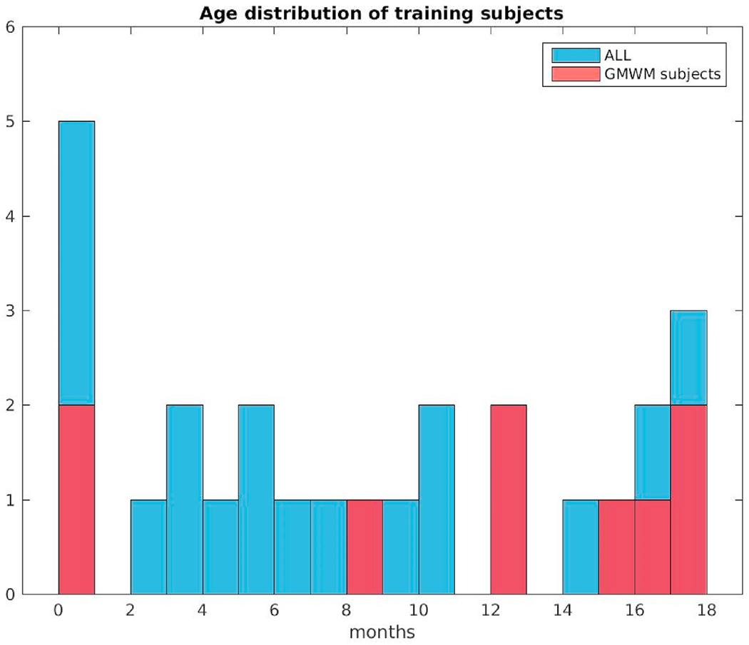
Age distribution at scan of the twenty-six subjects in the training data set. Red color indicates data samples that had GM/WM separation drawn by the manual labelers.
2.4.1.2. BCHneo.
For quantitative comparisons between our tool and others based solely on newborn datasets, we assembled a set of 17 healthy control neonates prospectively recruited at the BCH, independent of the training data set. Participating full-term neonates served for imaging purposes at 38.4 ± 1.4 weeks of gestational age, solicited from the well-baby units at our collaborating hospitals and imaged at 28.9 ± 10.5 days, with prior informed parental consent. They were all singletons with normal Apgar scores and no clinical concerns regarding perinatal brain injury or congenital or metabolic abnormalities. Of note, these data sets did not include corresponding full-brain manual segmentations.
2.4.2. Imaging acquisition
Scans of both BCH datasets were acquired using a 3 T MAGNETOM Trio Tim System or a 3 T MAGNETOM Skyra (Siemens Medical, Erlangen, Germany). Multi-echo volumetric magnetization prepared rapid gradient echo (MPRAGE) sequences (van der Kouwe et al., 2008) with volume navigators (vNav) for motion correction (Tisdall et al., 2012) (mocoMPRAGE) were obtained in the sagittal plane, at average image resolution of 1 mm3, using a 32-channel adult head coil (see Appendix Table 3 for more acquisition details). BCHneo newborns also had T2-weighted image acquisitions completed in the same sessions. All subjects were imaged during natural sleep, and all images were assessed for quality. Those scans considered unsuitable for segmentation, due to degradation by motion or other artifacts, were not included in above-described cohorts.
2.4.3. Skullstripping
Despite the challenges of skullstripping in an infant population, our tool achieved >90% overlap with expert-delineated brain masks (Ou et al., 2018), as measured by the Dice overlap coefficient (Dice, 1945). This performance is highly comparable to the long established adult skullstripping results of 94–96% (Roy et al., 2017). For volumes A and B with manually and automatically outlined ROIs, respectively,
| (5) |
where [A ∈ S] = {i ∈ I : A(i) ∈ S}. Representative skullstripping examples evaluated qualitatively are depicted in Fig. 4, including original unprocessed BCH_0–2yr images and their intensity-normalized and skullstripped versions. For easier visualization, these were all aligned using affine registration to an unbiased spatial coordinate system (Reuter et al., 2010, 2012; Aganj et al., 2015).
Fig. 4.
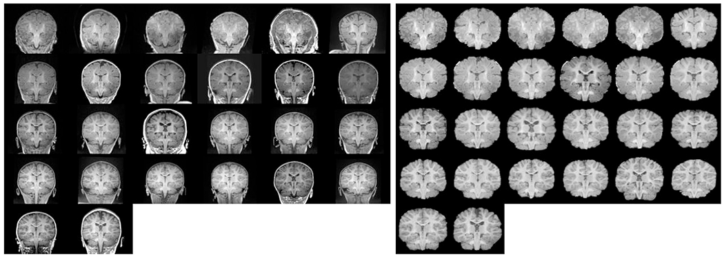
Skull-stripping results: (left) unprocessed images from BCH_0-2yr data set and (right) intensity normalized and skull-stripped results. Both sets are age sorted, displayed in coronal view and aligned using affine registration to an unbiased spatial coordinate space for easier visualization.
2.4.4. Automated vs manual volumetric segmentation
We used BCH_0-2yr, which includes manual segmentations, to quantitatively characterize our segmentation accuracy. Each infant brain MRI was used as a test image and was segmented using a subset of the remaining atlases. We identified training datasets by postnatal age to investigate (similar to others (Aljabar et al., 2009) (Gousias et al., 2013)) whether an age-related subset (vs the entire group) would be more accurate or efficient at the segmentation task. We varied the size of the training dataset from 1 to 25, proceeding from closest-in-age training subject to use of all the remaining datasets (excluding the test subject). Such age-dependent categories were motivated by a natural separation of the dataset, as well as by the fact that age matching of subjects would likely encourage more accurate segmentation results (Aljabar et al., 2009). In summary, this resulted in running N = 26 × 25 = 650 segmentation experiments. For all label-to-label comparisons, we computed both Dice (Dice, 1945; Zijdenbos et al., 1994) (corresponding to individual labels) and Generalized Dice (for overall accuracy) overlap coefficients of manually delineated and automatically outlined ROIs to quantify their agreement. For volumes A and B with manually and automatically outlined ROIs, respectively, the Generalized Dice score was computed as
| (6) |
where [A ∈ S] = {i ∈ I : A(i) ∈ S}. The Generalized Dice overlap coefficient was similarly defined in the generalized pair-wise multi-label Tanimoto Coefficient introduced by Crum et al. for fuzzy labels (Crum et al., 2006). We compared such measurements across the entire dataset, in smaller age-related subsets, and also across all training dataset sizes. We only computed overlap coefficients if both manual and automated segmentation solutions existed for a given ROI.
2.4.5. Automated volumetric segmentation comparison
No other infant brain segmentation tool described in the literature is able to segment single-channel T1-weighted images in our proposed age range. Therefore, to compare our segmentation outcomes both qualitatively and quantitatively, we segmented our prospectively collected dataset of newborns (BCHneo), having both T1- (T1w) and T2-weighted (T2w) images for each subject, using two other publically available tools: iBEAT (Wang, 2013, 2011b; Dai, n.d.) and MANTIS (Beare et al., 2016). We also processed T1-weighted structural images of the 40 subjects contained in the first release of The Developing Human Connectoe Project (Developing Human Connecto) as well as the ten training subjects from the iSEG2019 challenge (http://iseg2019.web.unc.edu/).
2.4.5.1. MANTIS.
MANTIS, the Morphologically Adaptive Neonatal Tissue Segmentation, extends the unified segmentation approach of tissue classification implemented in Statistical Parametric Mapping package (SPM (Penny et al., 2006)) to neonates. It utilizes a combination of unified segmentation, template adaptation via morphological segmentation tools and topological filtering, to segment the neonatal brain into eight tissue classes: cortical gray matter, white matter, deep nuclear gray matter, cerebellum, brainstem, cerebrospinal fluid (CSF), hippocampus and amygdala. This tool accepts brain-extracted T2-weighted images of newborns as inputs, so we used BET (Smith, 2002) processed T2w images from BCHneo. MANTIS does not make left/right hemispheric distinctions, so we combined our left and right labels (into a single label) for quantitative analysis. Label correspondences used for this analysis are outlined in Appendix Table 4.
2.4.5.2. iBEAT.
iBEAT, the Infant Brain Extraction and Analysis Toolbox, integrates several major functions for infant image analysis, including image preprocessing, brain extraction, tissue segmentation, and brain labeling. For brain extraction, a learning-based meta-algorithm, integrating a group of brain extraction results generated by two existing brain extraction algorithms (BET (Smith, 2002) and BSE (Shattuck et al., 2001)) is used; for segmentation of infant brain tissues, a level-sets-based tissue segmentation algorithm utilizing multimodality information, a cortical thickness constraint, and a longitudinal consistency constraint is implemented; and for labeling regions of interest of infant brain images, the HAMMER (Hierarchical Attribute Matching Mechanism for Elastic Registration) (Shen and DavatzikosHammer, 2002) registration algorithm warps pre-labeled ROIs of a template to the infant brain image space. This tool accepts corresponding T1w and T2w images as inputs, producing both subcortical and cortical segmentation labels. Although finding the anatomic correspondence between the subcortical labels of our tool and iBEAT was straightforward, that was not the case for cortical labels. Therefore, we have only provided qualitative and quantitative comparisons of subcortical ROIs. Label correspondences used for this analysis are outlined in Appendix Table 5.
2.4.5.3. dHCP.
Even though this consortium processed T2w images of 40 newborn subjects in its first release, the corresponding T1w images were also made available. We processed these images in our new pipeline (using the five newborn atlases in our training data), comparing our segmentation results to those derived by the dHCP pipeline (incorporating BET (Smith, 2002) and drawEM using T2w MRIs (Makropoulos et al., 2014)) relying on a set of mutually existing characterized labels. The original images of 0.8 × 0.8 × 0.8 mm3 were downsampled to 1-mm isotropic resolution for our processing. Given that no ground-truth registration files are available that define spatial correspondence between the T1-and T2-weighted images and the set of overlapping segmentation labels common in the outputs of both pipelines is relatively low, we have only provided a qualitative segmentation comparison.
2.4.5.4. iSEG.
We have also downloaded the training data set corresponding to the iSEG2019 MICCAI challenge. It contains T1-and T2-weighted MRI images of 10 6-month old subjects along with manual segmentations of three regions of interest: GM, WM and CSF. The MRI data is of 1-mm isotropic resolution, already skullstripped and do not include the brainstem or cerebellum regions. For further details, see (al, 2019). In order to adapt to these type of input images, we carried out two different types of experiments. (A) We modified our training data set in a way that we masked out the brainstem and cerebellar areas from all. Then we ran our full pipeline with neighborhood sizes of 1–12. After the completion of each run we combined our output labels in order to match those of iSEG and used those for computing overlap accuracy. Label correspondences used for this analysis are outlined in Appendix Table 6. (B) We also ran the segmentation part of our pipeline in a way that our training data was replaced by the iSEG image set. We used neighborhood sizes of 1–9 (never using the test data itself in the training data) and computed Dice overlap coefficients with respect to the iSEG-provided segmentations.
3. Results
A detailed report of the inter-rater variability measures of the manual segmentation of our training set can be found elsewhere (de Macedo Rodrigues et al., 2015). In brief, we reported results from two independent inter-rater variability studies. One showed that the worst performance (<60%), with respect to Dice overlap measures, was observed in the case of the L Amygdala. In the other study, L and R Accumbens performed worst (<50%), and there were nine labels where overlap was >80% (L/R Thalamus, L/R Caudate, L/R Putamen, Vermis, Midbrain, and Pons).These values represent an upper bound for the performance achievable by our automated pipeline.
3.1. Qualitative segmentation evaluation
We first demonstrated the quality of our automated segmentation using a set of five representative and variably aged subjects (newborn, 8 mo, 12 mo, 16 mo, and 18 mo), displaying both manually and automatically labeled brain images. Fig. 5 shows selected snapshots of these subjects in coronal views, with the input image, the manually segmented solution, and its outline (overlain on input image), plus the corresponding segmentation and its outline (overlain on input image) in 5 respective columns. In the first row, input images of a newborn clearly display the reverse intensity contrast of an adult. However, in other subjects of the remaining rows, the intensity contrast more closely resembled that of an adult, albeit with unmyelinated areas still visible. In all of these images, GM/WM boundaries and subcortical region segmentations demonstrate high levels of correspondence. Of note, WM of cerebellum was not included in manual segmentation of the newborn or the 12 month-old and thus is missing from the second-row display.
Fig. 5.

Five automated segmentation examples where manual segmentation also contained GM/WM separation: (from top to bottom) newborn, 8mo, 12mo, 16mo, 18mo. From left to right: normalized and skullstripped T1-weighted input image, manual segmentation, manual segmentation outline, automated segmentation, automated segmentation outline. All segmentations (or their outlines) are overlaid on the normalized and skullstripped T1-weighted input image. The segmentation colors correspond to the default Freesurfer colortable.
In Fig. 6, we have shown another set of representative images from five other subjects aged 2, 3, 5, 6, and 9 months. In these subjects, manual segmentations did not include the GM/WM boundaries due to uncertain contrast intensity. However, the automated tool still recovered white matter segmentation labels with acceptable accuracy in the majority of the cases, when comparing images with WM-labeled training subjects of similar ages.
Fig. 6.
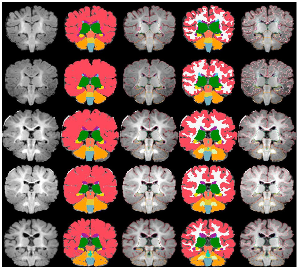
Five automated segmentation examples where manual segmentation did not contain GM/WM separation: (from top to bottom) 2mo, 3mo, 5mo, 6mo, 9mo. From left to right: normalized and skull-stripped T1-weighted input image, manual segmentation, manual segmentation outline, automated segmentation, automated segmentation outline. All segmentations (or their outlines) are overlaid on the normalized and skull-stripped T1-weighted input image. The segmentation colors correspond to the default Freesurfer colortable.
3.2. Quantitative segmentation evaluation
Fig. 7 is a graph of Generalized Dice overlap coefficients for all 26 subjects evaluated in BCH_0–2yr over training set sizes of 1–25, selected by age. The subjects are presented by age in ascending order (dark blue indicating the youngest subject and bright yellow indicating the oldest). The highest measurements are attributable to subjects in the middle of our age range of interest, whereas the lowest are those of newborns. We must also acknowledge that in all cases, use of a subset rather than the complete training set, yielded better overall segmentation performance. This may be explained by age differences in the training dataset. Such trends are even more obvious when we display our overlap measures for five non-overlapping age groups across the increasing training set sizes: newborns (N = 5), 2–4 mo (N = 4), 5–8 mo (N = 5), 9–14 mo (N = 6), and 15–18 mo (N = 6). Fig. 8 shows the average and Fig. 9 the maximum Generalized Dice measures for these age groups. In the former, the highest values reached 0.83; but in the latter, a value of nearly 0.94 was recorded.
Fig. 7.

Generalized Dice overlap coefficient summary for all subjects and training set sizes (selected by age). The generalized Dice coefficients are displayed for training set sizes 1–25 for all of our subjects, in an age-sorted manner: Subj8 (newborn) → Subj 25 (18 mo).
Fig. 8.
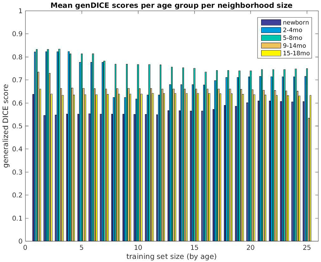
Mean generalized Dice overlap coefficient summary over all training set sizes (selected by age) for all subjects, grouped into five non-overlapping age groups (newborns (N = 5), 2–4 month (N = 4), 5–8 month (N = 5), 9–14 month (N = 6) and 15–18 month olds (N = 6)). The measures are displayed for training set sizes 1–25.
Fig. 9.
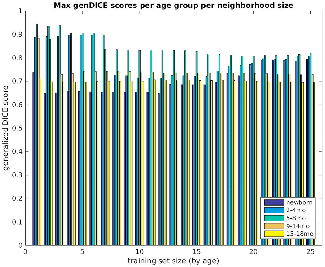
Maximum generalized Dice overlap coefficient over all training set sizes (selected by age) for all subjects grouped into five non-overlapping age groups (newborns (N = 5), 2–4 month (N = 4), 5–8 month (N = 5), 9–14 month (N = 6) and 15–18 month olds (N = 6)). The measures are displayed for training set sizes 1–25.
To quantify which neighborhood size in the label fusion algorithm yields the best segmentation performance, we have shown (Fig. 10) the number of times a particular neighborhood size prevailed as best performer (using overall Dice overlap coefficients) across the five age groups. There is ample clustering of winning numbers under the size 5 training dataset. Fig. 11 displays the Generalized Dice overlap score versus age-at-scan computed on the training data set for this neighborhood size.
Fig. 10.
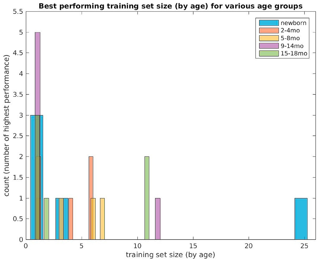
Best performing training set sizes (selected by age) computed using generalized Dice coefficients in five non-overlapping age categories (newborns (N = 5), 2–4 month (N = 4), 5–8 month (N = 5), 9–14 month (N = 6) and 15–18 month olds (N = 6)).
Fig. 11.

Generalized Dice score vs age-at-scan computed on the training data set for neighborhood size 5.
In Supplementary Figures 2–4, average Dice scores per segmentation ROIs are depicted over all subjects in BCH_0–2yr, with respect to training set sizes of 1–12 (selected by age). The highest score was consistently achieved in L/R Thalamus and Pons regions.
3.3. Qualitative and quantitative comparisons with other tools
As discussed above, a fair direct comparison of these tools/datasets (with differing input image requirements and differing segmentation label sets) is not feasible. Nevertheless, we examined their segmentation outcomes to better appreciate the inherent disparities and the difficulty in absolute ranking of tools. Note, no manual labels were available for the below testing data sets, so the segmentation outcomes were just directly compared to each other and not to ground truth.
We ran MANTIS (Beare et al., 2016) on T2w images of 17 newborns (GA, 38.7 ± 1.2 wks; age at scan, 28.2 ± 11.4 days) and our segmentation pipeline using corresponding T1w images, comparing commonly identified segmentation labels. The list of such ROIs included cerebral cortex, cerebral white matter, deep gray matter, hippocampus, amygdala, cerebellum, and brainstem. MANTIS does not distinguish between left and right hemispheric labels, so for sake of comparison, we merged our hemispheric labels. We have shown coronal views of input images and segmentation outcomes (affinely aligned for visualization purposes) in Fig. 12. In Fig. 13, Dice overlap measures computed for corresponding labels are plotted for each subject. The overall match between these segmentation solutions was 0.7–0.8, with brainstem, cerebellum, and deep gray matter closer to 0.8 and hippocampus and amygdala often <0.5.
Fig. 12.
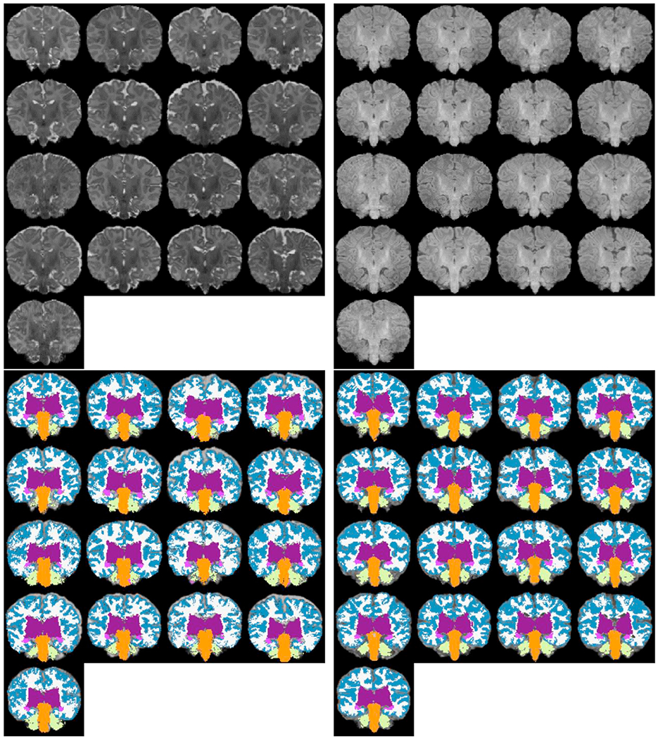
MANTIS segmentation comparison: (top left) T2w input images (bottom left) MANTIS segmentations, (top right) corresponding T1w input images (bottom right) our segmentation outcome after grouping left/right hemisphere labels together. The list of commonly identified labels are: cerebral cortex, cerebral white matter, deep gray matter, hippocampus, amygdala, cerebellum and brainstem. For more detailed label correspondences see Appendix Table 4.
Fig. 13.
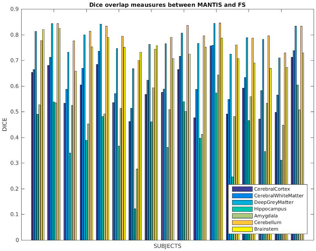
Dice coefficients computed between our segmentations and MANTIS for labels that are commonly identified by these tools: cerebral cortex, cerebral white matter, deep gray matter, hippocampus, amygdala, cerebellum and brainstem.
We also ran iBEAT (Dai, n.d.) on a set of twelve matching T1w and T2w images of newborns (GA, 38.7 ± 1.4 wks; age at scan, 29.75 ± 11 days) and our segmentation pipeline on their corresponding T1w images and compared the commonly identified labels in the outcomes. In our qualitative and quantitative comparison we only include the commonly defined subcortical labels: left/right thalamus, caudate, putamen, pallidum, hippocampus, and amygdala. We display a coronal view of the input T1w images and the segmentation outcomes (affinely aligned for visualization purposes) in Fig. 14. Fig. 15 shows Dice overlap measures computed between corresponding labels for each subject. There are no labels that seem to consistently perform better or worse, but the amygdala, putamen and hippocampus produce higher matches in some cases. The overall match between these labels, however, is lower, around 0.6.
Fig. 14.

iBEAT subcortical segmentation comparison: (left) T1w input images (middle) iBEAT segmentations, (right) our segmentation outcome. The list of commonly identified labels are: left/right thalamus, caudate, putamen, pallidum, hippocampus and amygdala. For more detailed label correspondences see Appendix Table 5.
Fig. 15.
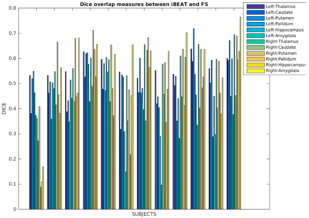
Dice coefficients computed between our segmentations and iBEAT for labels that are commonly identified by these tools: left/right thalamus, caudate, putamen, pallidum, hippocampus and amygdala.
We used our new segmentation tool to process images of the 40 subjects in the 1st dHCP data release (Developing Human Connecto). Coronal views of the input T1w images, our skull-stripping solutions, and our segmentation outcomes (affinely aligned for visualization purposes) are shown in Figs. 16 and 17, with all commonly identified ROIs: left/right cortical gray matter, cortical white matter, ventricles, hippocampus, amygdala, caudate, thalamus, and lateral ventricles, as well as the cerebellum and brainstem. Fig. 18 shows T2w input images of the dHCP and their segmentation solutions. Overall, the dHCP cortical segmentations seem slightly more accurate. One key explanation for this is the discrepancy in qualities of T1w and T2w input images (for example, second row 1st or third row 3rd and 4th images at tops of Figs. 17 and 18).
Fig. 16.
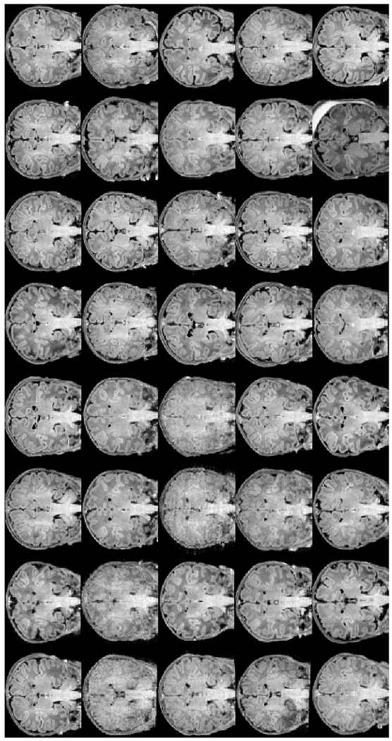
T1w input images of the first forty subjects constituting the recent data elease of the “The Developing Human Connectoe Project” dHCP project viewed in the coronal plane in an unbiased common affine coordinate system.
Fig. 17.
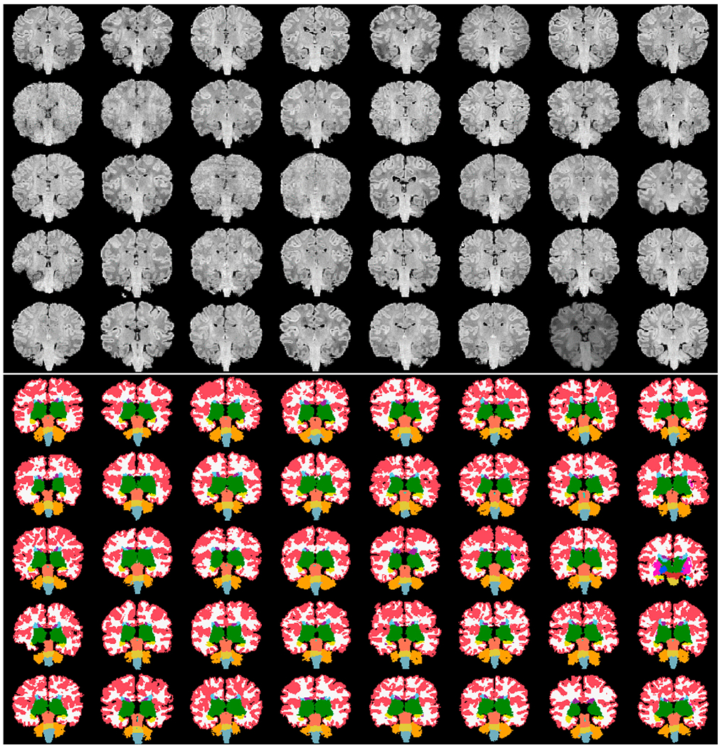
The first forty subjects constituting the recent data release of the “The Developing Human Connectoe Project” dHCP project viewed in the coronal plane in an unbiased common affine coordinate system: (top) skull-stripped input images, and (bottom) segmented images using our new pipeline.
Fig. 18.

The first forty subjects constituting the recent data release of the “The Developing Human Connectoe Project” dHCP project viewed in the coronal plane in an unbiased common affine coordinate system: (top) original T2w input images, and (bottom) dHCP released tissue segmentation outcomes (based on T2w images).
Fig. 19 displays Mean Dice overlap measures computed on this dataset per segmentation labels between our and the dHCP processing pipeline. The nomenclature originates from the data released by the dHCP consortium: “all” identifying 13 labels in total and “tissue” segmentation labels referring to more detailed segmentation results, but only 7 of them overlapping with our definitions.
Fig. 19.
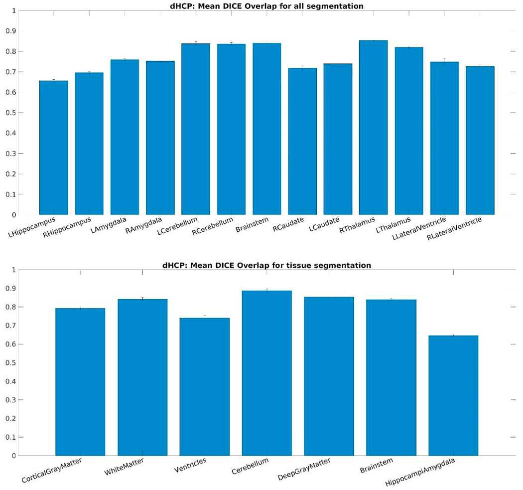
Mean Dice overlap measures computed on the DHCP dataset per segmentation labels: (top) “all” segmentation labels and (bottom) “tissue” segmentation labels released by the dHCP consortium.
Quantitative results from our iSEG experiments are displayed in Fig. 20. We computed Dice overlap measures on the 10 training subjects of the iSEG data set per segmentation labels. The top plot displays outcomes from experiment A (modified pipeline with our own training data set) using neighborhood sizes 1–12 and the bottom one shows those from experiments B (our proposed segmentation with iSEG training data) using neighborhood sizes 1–9. Note, as the training data set in our proposed pipeline does not include a label for CSF, for experiments (A), we computed overlap measurements for GM and WM only. Even though our own training data set contains several subjects around the isointense phase that is represented by iSEG, only one, the 8-month-old, has GM/WM separation. The lack of representation with GM/WM separation of this particular age explains the max 78 and 66% overlap accuracy and the fact that the performance of the pipeline declines with larger neighborhood sizes. For experiments B, the highest performance was reached by using neighborhood size of 9 (75,77 and 73% for CSF, GM and WM), but the performance does not seem to have plateaued, suggesting that for this particular age, and using only the T1-weighted input images as inputs a larger training data set could result in even higher performance when using the multi-label fusion segmentation approach of our proposed pipeline.
Fig. 20.

Mean Dice overlap measures computed on the 10 training subjects of the iSEG data set per segmentation labels: (top) the proposed pipeline was run after eliminating the brainstem and cerebellum and segmentation labels combined to match those included in iSEG using neighborhood size 1–12 and (bottom) the volumetric segmentation part of our proposed pipeline was run using the iSEG training data set using neighborhood size 1–9.
3.4. Surface extraction
Due to lack of ground-truth surface reconstruction of our input images we first display surfaces for qualitative evaluation. In Fig. 21, representative surface models of five subjects (newborn, 8, 12, 16, and 18 months old) are shown. The surfaces are those of white matter, pia, and a spherical representation with curvature-map overlay. In addition to a qualitative evaluation, we also performed a set of quantitative quality control tests. On a scale of 0–5, two independent experts scored the quality of white matter and pial surface reconstructions of the same five subjects appearing in Fig. 21, deducting scores from maximum for errors such as holes, mislabeled ventricles, dura grabbing, or missed gyri. Both evaluations resulted in average surface scores of 3, with standard deviations of 0.7 and 0.8. Detailed outcomes of this analysis are provided in Supplementary Figure 5.
Fig. 21.
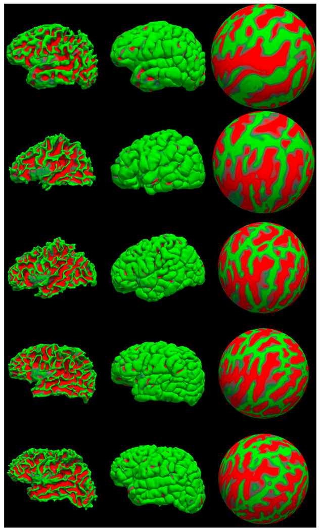
Surfaces generated for five sample subjects from our training dataset: (from top to bottom) newborn, 8mo, 12mo, 16mo, 18mo. From left to right: left hemisphere white surface, pial surface and spherical representation with a curvature map overlay.
On the dHCP data set we also compared the surfaces provided by the dHCP pipeline to our proposed outcomes. Fig. 22 displays a comparison between surface measurements per hemispheres. We computed the mean absolute distance between the two sets of solutions as well as the mean sulcal depth, cortical thickness and curvatures differences. In summary, these differences were on average 1.17 mm, −0.5, 0.9 and −0.09, respectively. The more detailed, per cortical parcellation label comparison of these measurements is included in Supplementary Figure 6.
Fig. 22.

Boxplot displays comparing surface measures on the dHCP data set, per hemisphere, all labels combined: (top left) mean absolute distance, (top right) mean sulcal depth difference, (bottom left) mean cortical thickness difference and (bottom right) mean curvature differences.
Additionally, we randomly selected 12 and 10 subjects, respectively, from the BCH_0–2 years and dHCP data sets and a trained expert drew points on the white matter and pial surfaces based on their T1 weighted MRI. On average 75 control points were placed on both of these surfaces, on both hemispheres (see Fig. 23, for an example). We then computed the shortest distance between these points and our computed surfaces. Additionally, in the case of the dHCP dataset, we also computed distances between the manually drawn points and surfaces provided by the dHCP minimal processing pipeline. The mean and standard deviation of the absolute value of these measurements are included in Table 2. The white matter surfaces tend to be slightly higher in the case of our proposed method, while in the case of the dHCP pipeline it is the pial surface differences that are higher. On the studied dHCP data set, the minimal processing pipeline outperforms our solutions with a statistically significant difference at the 5% significance level.
Fig. 23.
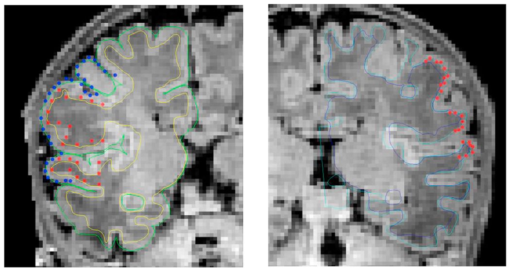
Examples of validation surface points placed on the right and left hemispheres of a randomly selected T1 weighted image from the dHCP data set, viewed on different coronal slices. (Left) validation surface points from both the pial (blue) and white (red) surfaces are shown along with our surface reconstruction solutions (light green – pial surface, yellow – white matter surface); (Right) validation surface points from the white (red) surface are shown along with the dHCP and our white matter surface reconstruction solutions (light blue – dHCP, dark blue – ours).
Table 2.
Surface to label distances computed on two data sets (BCH0–2 years and dHCP data set). Using 12 and 10 randomly selected subjects, respectively, shortest distances between points identified in the T1-weighted volume and the reconstructed surfaces were computed and the mean and standard deviation of the absolute value of these measurements are included in the Table.
| Infant FS | dHCP | ||
|---|---|---|---|
| BCH_0–2 years | White matter surface | 1.1732 (1.2525) | N/A |
| Pial surface | 0.9198 (0.9054) | N/A | |
| dHCP | White matter surface | 1.1898 (1.1468) | 0.4585 (0.3384) |
| Pial surface | 0.8070 (0.8358) | 0.6470 (0.5205) |
4. Discussion
4.1. General comments
We have introduced an automated segmentation and surface extraction pipeline for image processing in infants designed to accommodate clinically acquired infant brain MRI data from a population of 0–2 year-olds. To our knowledge, there is no algorithm or computational pipeline capable of consistently handling single time-point T1-weighted MR images of subjects within this postnatal period, producing full-brain volumetric segmentations and surface extractions. The innovative aspect of this method resides in the adaptation of three key methodological solutions that aggregate infant MRIs in a pipeline for thorough evaluation. These key components are a manually segmented training dataset for the age range of interest, a robust skull-stripping algorithm, and a multi-atlas label-fusion segmentation framework benefitting from information encoded in the training set and the surface extractions. The primary advantage of our algorithm is that it can be optimized for any age. Indeed, the pipeline selects a subset of the training dataset most similar to the target subject to generate segmentations and surfaces.
Through our experimentation, we presented both qualitative and quantitative evaluations to characterize the performance of our tool, showing that its overall functioning was consistent across the target age range; and its accuracy (as measured by Dice and Generalized Dice coefficients) was high for such a difficult task. The highest mean and maximum generalized Dice overlap coefficient scores were obtained for the 2–8 mo subset and the lowest for the newborns. We also investigated whether age-dependent sub-grouping of the manually segmented datasets would be beneficial and found that a training dataset of few atlases close in age to test subjects was optimal. Observations on diminishing returns and worsening performance of an enlarging training dataset may have validity in this instance, serving to increase the diversity of the training data. The more training subjects used, the larger the age disparity between the test subject and at least some training subjects. However, those subjects deviating substantially from the test subject, may not contribute significantly to segmentation accuracy owing to information conflicts with closer-in-age subjects and possibly higher registration inaccuracies. Note also that we ran the same number of experiments for training-set size selection, using mutual information (MI)-based criteria and focusing on image similarity, as opposed to aligning subjects with atlases by age. In a majority of cases, age-related selection performed superiorly, which is why we omitted performance metrics for the MI-based experiments conducted. We believe that performance discrepancies are readily explained by the fact that for our normal control group, age was a robust and reliable parameter determining structural similarities of input images. However, in the presence of disease this may not be true, so image-based selection criteria will also be available in our forthcoming software release.
We likewise compared our segmentation solutions both qualitatively and quantitatively to three other publically available algorithms based on newborn training datasets. The overall correspondence between such outcomes was generally good but was also quite varied, showing perhaps the best correspondence with dHCP results. However, due to differences in label definitions, as well as shifting requirements and quality of input images, such comparisons should be further investigated moving forward.
Motion artifacts have a great impact on infant image quality. It is almost impossible, however, to quantify the amount of motion in a scan if no steps had been taken during the acquisition stage to save related information (such as head tracking). Given that we used retrospectively selected data sets in this study, we had no such information at hand. As an alternative, we computed a reference-free measure of image sharpness, the Tenengrad metric from (Kecskemeti et al., 2018), in order to quantitatively characterize the quality of our data sets. We computed this metric in the common affine (visualization) space based on the middle slice of the image volume. First we point out the close relationship between the age-at-scan and the Tenengrad metric displayed in Fig. 24. As the former gets higher, the sharpness metric also tends to increase. Second, Fig. 25 displays the Generalized Dice score for each of training subjects using 4 and 5 as training neighborhood sizes vs the input image volumes’ Tenengrad metric (fmeasure). This figure demonstrates a clear tendency for a higher Generalized Dice score associated with a higher sharpness metric (and higher age-at-scan).
Fig. 24.
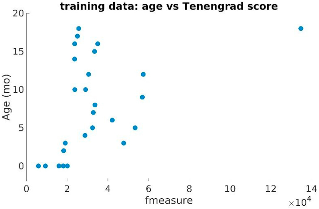
Age-at-scan vs the Tenengrad image sharpness metric (fmeasure) computed on the training dataset (BCH0–2 years).
Fig. 25.
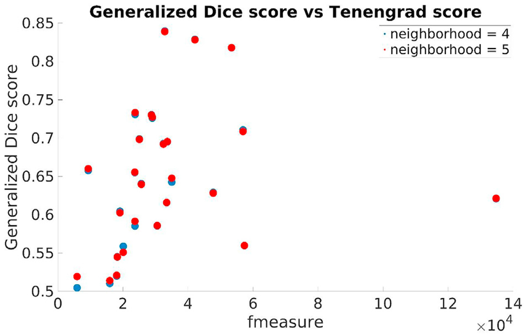
Generalized Dice score for each of training subjects using 4 and 5 as training neighborhood sizes vs the input image volumes’ Tenengrad metric (fmeasure).
The Tenengrad image sharpness metric for the dHCP newborns on the T1-weighted images was in the same range as that of those of the newborn training subjects. Fig. 26 displays this score along with the Generalized Dice score using a training neighborhood size of 5: “all” segmentation labels (in red) and common-with-our-pipeline “tissue” labels (in blue).
Fig. 26.
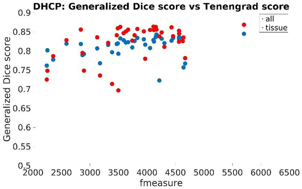
Generalized Dice score for each of dHCP subject using 5 as training neighborhood sizes vs the input image volumes’ Tenengrad metric (fmeasure): “all” (in red) and common-with-our-pipeline “tissue” labels (in blue).
The segmentation and image processing pipeline described in this paper will be distributed in source and binary format under the existing FreeSurfer platform and under a modified MIT-style license (FreeSurfer Software Licen), in conjunction with our training dataset.
4.2. Limitations
Current limitations of our image processing solution stem from the fact that our proposed pipeline as yet does not accommodate T2w MRI images, which typically confer higher CNRs for infants up to 6 months of age (Dubois et al., 2014). This limits our ability to directly compare the performance of our application with that of existing tools, particularly in terms of the newborn sub-population. At the same time, we also fill a void in the literature, providing a tool for researchers and clinicians who use more clinically practical 2D T2w images (rather than longer, high-resolution isotropic T2w images) in regular patients but generally acquire faster volumetric T1w images for clinical studies. The current pipeline resamples all input images to be 1 mm isotropic in order to match the resolution of the training data sets. In the future, we aim to remove this constraint by obtaining higher resolution manually segmented data sets for both training and validation. In their present state, our tools may already generate a set of cortical parcellations analogous to those of the FreeSurfer adult pipeline, but we did not characterize them in this paper. Finally, the current training dataset is missing some GM/WM boundary descriptions. We feel that increasing the number of training subjects, gathering full GM/WM segmentations across the entire age range will further increase the accuracy and consistency of our segmentation and surface extraction outcomes.
4.3. Future initiatives
The current pipeline provides an excellent platform for future extensions as follows: (i) A planned extension of our segmentation and skullstripping training datasets using T2w samples, potentially enhancing segmentation accuracy in newborn populations and allowing direct comparisons of our performance with outcomes of other publically available image-processing tools and multi-site datasets: The emergence and public sharing of datasets through initiatives such as dHCP (available at http://www.developingconnectome.org/) and MICCAI challenge datasets (available at http://neobrains12.isi.uu.nl, http://iseg2017.web.unc.edu/and http://iseg2019.web.unc.edu/) will be instrumental in this regard; (ii) Full use of the thoroughly tested FreeSurfer framework (consistently handling analysis of longitudinal images (Reuter et al., 2012; Reuter and Fischl, 2011)) to potentially increase the sensitivity/specificity of follow-up group analyses and require fewer subjects to detect comparable effect sizes (Reuter et al., 2012; Reuter and Fischl, 2011): The FreeSurfer implementation of longitudinal processing is somewhat similar to that of Shi et al. (2010), without favoring any of the time points, which may lead to bias and encourage spurious effects (Reuter and Fischl, 2011; Yushkevich et al., 2010); (iii) Annotation of cortical parcellation areas, specifically in our population of interest, on surfaces that are currently extracted from our volumes and include those references within our pipeline: This would provide a new infant-specific set of labels comparable to the recent release by Alexander et al. defined on T2w images for newborns (Alexander et al., 2017; Alexander B et al., 2019); (iv) Emphasis on performance in cortical surface placement: Cortical thickness is a powerful biomarker that has been used in many clinical studies to assess of a variety of neurologic and neuro-developmental outcomes (McCauley et al., 2010; Almeida et al., 2010; Kirk et al., 2009; Wolosin, 2009; Merkley, 2008). In the future, we plan to manually estimate cortical thickness, comparing resultant values with measures reported in the literature; and (v) The emergence of neural network-based image analysis frameworks, in particular solutions estimating deformable templates, creates an exciting opportunity to incorporate efficient learning solutions, such as conditional atlases (Dalca et al., 2019), into our infant brain analysis pipeline.
Supplementary Material
Acknowledgements
Support for this research was provided in part by NIH/NICHD grants 1K99HD061485-01A1, R00 HD061485-03, 5R03EB022754-02, 5R21HD95338-02, 5R01HD085813-04, 5R01 HD065762-09, 5R01HD093578-03, 5R01EB024343-03 (LZ); A. A. Martinos Center Computing facilities: NIH S10RR023401, S10RR019307, S10RR019254, S10RR023043; NIH/NIBIB grants P41EB015896, 1R01EB023281, R01EB006758, R21EB018907, R01EB019956, NIH/NIA grants 1R56AG064027, 5R01AG008122, R01AG016495, NIH/NIDDKD grant 1-R21-DK-108277-01, NIH/NINDS R01NS0525851, R21NS072652, R01NS070963, R01NS083534, 5U01NS086625, the NIH Blueprint for Neuroscience Research (5U01-MH093765), part of the multi-institutional Human Connectome Project (BF); the European Research Council (Starting Grant 677697, project BUNGEE-TOOLS) (JEI); NIH R01HD076258 (PEG); NIH R01EB014947 (YO, PEG); Thrasher Early Career Development Grant (YO); as well as partially from Abbott Nutrition through the Center for Nutrition, Learning, and Memory at the University of Illinois (trial being registered at clinicaltrials.gov as NCT02058225). In addition, BF has a financial interest in CorticoMetrics, a company whose medical pursuits focus on brain imaging and measurement technologies. BF’s interests were reviewed and are managed by Massachusetts General Hospital and Partners HealthCare in accordance with their conflict-of-interest policies. Finally, the authors would like to acknowledge the meticulous and detail-oriented work of several students and research assistants who assisted us with analysis of the above described dataset: Rutvi Vias, Christopher Ha, Lucy Schlink, and Ngo Giang-Chau.
Footnotes
Appendix A. Supplementary data
Supplementary data to this article can be found online at https://doi.org/10.1016/j.neuroimage.2020.116946.
References
- Aganj I, et al. , 2015. Avoiding symmetry breaking spatial non-uniformity in deformable image registration via a quasi-volume-preserving constraint. Neuroimage 106, 238–251. [DOI] [PMC free article] [PubMed] [Google Scholar]
- al W.e., 2019. Benchmark on automatic six-month-old infant brain segmentation algorithms: the iSeg-2017 challenge. IEEE Trans. Med. Imag. 38 (9), 2219–2230. [DOI] [PMC free article] [PubMed] [Google Scholar]
- Alexander B LW, Matthews LG, Murray AL, Adamson C, Beare R, Chen J, Kelly CE, Anderson PJ, Doyle LW, Spittle AJ, Cheong JLY, Seal ML, Thompson DK, 2019. Desikan-killiany-tourville atlas compatible version of M-CRIB neonatal parcellated whole brain atlas: the M-CRIB 2.0. Front. Neurosci. 13 (34). [DOI] [PMC free article] [PubMed] [Google Scholar]
- Alexander B, et al. , 2017. A new neonatal cortical and subcortical brain atlas: the Melbourne Children’s Regional Infant Brain (M-CRIB) atlas. Neuroimage 147, 841–851. [DOI] [PubMed] [Google Scholar]
- Aljabar P, et al. , 2009. Multi-atlas based segmentation of brain images: atlas selection and its effect on accuracy. Neuroimage 46 (3), 726–738. [DOI] [PubMed] [Google Scholar]
- Almeida LG, et al. , 2010. Reduced right frontal cortical thickness in children, adolescents and adults with ADHD and its correlation to clinical variables: a cross-sectional study. J. Psychiatr. Res. 44, 1214–1223. [DOI] [PubMed] [Google Scholar]
- Bastiani M, Andersson JLR, Cordero-Grande L, Murgasova M, Hutter J, Price AN, Makropoulos A, Fitzgibbon SP, Hughes E, Rueckert D, Victor S, Rutherford M, Edwards AD, Smith SM, Tournier J-D, Hajnal JV, Jbabdi S, Sotiropoulos SN, 2019. Automated processing pipeline for neonatal diffusion MRI in the developing Human Connectome Project. Neuroimage 185, 750–763. [DOI] [PMC free article] [PubMed] [Google Scholar]
- Beare RJ, et al. , 2016. Neonatal brain tissue classification with morphological adaptation and unified segmentation. Front. Neuroinf. 10 (12). [DOI] [PMC free article] [PubMed] [Google Scholar]
- Bellinger DC, et al. , 2003. Neurodevelopmental status at eight years in children with dextro-transposition of the great arteries: the Boston Circulatory Arrest Trial. J. Thorac. Cardiovasc. Surg. 126, 1385–1396. [DOI] [PubMed] [Google Scholar]
- Cachia A, et al. , 2003. A primal sketch of the cortex mean curvature: a morphogenesis based approach to study the variability of the folding patterns. IEEE Trans. Med. Imag. 22 (6), 754–765. [DOI] [PubMed] [Google Scholar]
- Crum W, Camara O, Hill DLG, 2006. Generalized overlap measures for evaluation and validation in medical image analysis. IEEE Trans. Med. Imag. 25 (11), 1451–1461. [DOI] [PubMed] [Google Scholar]
- D Rex DS, Woods R, et al. , 2004. A meta-algorithm for brain extraction in MRI. Neuroimage 23 (2), 625–637. [DOI] [PubMed] [Google Scholar]
- Dai Y, Shi F, Wang L, Wu G, Shen D, April 2013. iBEAT: A Toolbox for Infant Brain Magnetic Resonance Image Processing. Neuroinformatics 11 (2), 211–225. [DOI] [PubMed] [Google Scholar]
- Dalca AV, et al. , 2019. Learning Conditional Deformable Templates with Convolutional Networks arXiv.org > cs > arXiv:1908.02738. [Google Scholar]
- Dale AM, Sereno MI, 1993. Improved localization of cortical activity by combining EEG and MEG with MRI cortical surface reconstruction: a linear approach. J. Cognit. Neurosci. 5 (2), 162–176. [DOI] [PubMed] [Google Scholar]
- Dale AM, Sereno MI, 1993. Improved localization of cortical activity by combining EEG and MEG with MRI cortical surface reconstruction: a linear approach. J. Cognit. Neurosci. 5, 162–176. [DOI] [PubMed] [Google Scholar]
- Dale AM, Fischl B, Sereno MI, 1999. Cortical surface-based analysis I: segmentation and surface reconstruction. Neuroimage 9, 179–194. [DOI] [PubMed] [Google Scholar]
- de Macedo Rodrigues K, et al. , 2015. A FreeSurfer-compliant consistent manual segmentation of infant brains spanning the 0–2 year age range. Front. Hum. Neurosci 9 (21). [DOI] [PMC free article] [PubMed] [Google Scholar]
- Dehaene-Lambertz G, Dehaene S, Hertz-Pannier L, 2002. Functional neuroimaging of speech perception in infants. Science 298, 2013–2015. [DOI] [PubMed] [Google Scholar]
- Desikan RS, et al. , 2006. An automated labeling system for subdividing the human cerebral cortex on MRI scans into gyral based regions of interest. Neuroimage 31 (3), 968–980. [DOI] [PubMed] [Google Scholar]
- Developing human connectome project. Available from: http://www.developingconnectome.org.
- Dice LR, 1945. Measures of the amount of ecologic association between species. Ecology 26, 297–302. [Google Scholar]
- Doshi J, et al. , 2013. Multi-atlas skull-stripping. Acad. Radiol. 20 (12), 1566–1576. [DOI] [PMC free article] [PubMed] [Google Scholar]
- Dubois J, et al. , 2008. Mapping the early cortical folding process in the preterm newborn brain. Cerebr. Cortex 18, 1444–1454. [DOI] [PubMed] [Google Scholar]
- Dubois J, et al. , 2014. The early development of brain white matter: a review of imaging studies in fetuses, newborns and infants. Neuroscience 276 (C), 48–71. [DOI] [PubMed] [Google Scholar]
- Ecker C, et al. , 2009. Is there a common underlying mechanism for age-related decline in cortical thickness? Neuroreport 20 (13), 1155–1160. [DOI] [PubMed] [Google Scholar]
- Elad A, Keller Y, Kimmel R, 2005. Texture mapping via spherical multidimensional scaling In: Scale-Space Theories in Computer Vision. Scale-Space 2005. Lecture Notes in Computer Science, 3459 Springer, Berlin, Heidelberg. [Google Scholar]
- Fischl B, 2012. FreeSurfer. NeuroImage 62 (2), 774–781. [DOI] [PMC free article] [PubMed] [Google Scholar]
- Fischl B, Dale AM, 2000. Measuring the thickness of the human cerebral cortex from magnetic resonance images. Proc. Natl. Acad. Sci. Unit. States Am 97, 11044–11049. [DOI] [PMC free article] [PubMed] [Google Scholar]
- Fischl B, Dale A, 2000. Measuring the thickness of the human cerebral cortex from magnetic resonance images. Proc. Natl. Acad. Sci. U.S.A 97, 11044–11049. [DOI] [PMC free article] [PubMed] [Google Scholar]
- Fischl B, Sereno MI, Dale AM, 1999. Cortical surface-based analysis II: inflation, flattening, and a surface-based coordinate system. Neuroimage 195–207. [DOI] [PubMed] [Google Scholar]
- Fischl B, et al. , 1999. High-resolution inter-subject averaging and a coordinate system for the cortical surface. In: Human Brain Mapping, pp. 272–284. [DOI] [PMC free article] [PubMed]
- Fischl B, Sereno MI, Dale AM, 1999. Cortical surface-based analysis II: inflation, flattening, and a surface-based coordinate system. Neuroimage 195–207. [DOI] [PubMed] [Google Scholar]
- Fischl B, Sereno MI, Dale AM, 1999. Cortical surface-based analysis II: inflation, flattening, and a surface-based coordinate system. Neuroimage 9 (2), 195–207. [DOI] [PubMed] [Google Scholar]
- Fischl B, et al. , 1999. High-resolution inter-subject averaging and a coordinate system for the cortical surface. Hum. Brain Mapp. 8 (4), 272–284. [DOI] [PMC free article] [PubMed] [Google Scholar]
- Fischl B, Liu A, Dale AM, 2001. Automated manifold surgery: constructing geometrically accurate and topologically correct models of the human cerebral cortex. IEEE Trans. Med. Imag. 20 (1), 70–80. [DOI] [PubMed] [Google Scholar]
- Fischl B, et al. , 2002. Whole brain segmentation: automated labeling of neuroanatomical structures in the human brain. Neuron 33 (3), 341–355. [DOI] [PubMed] [Google Scholar]
- Fischl B, et al. , 2004. Sequence-independent segmentation of magnetic resonance images. Neuroimage 23 (Suppl. 1), S69–S84. [DOI] [PubMed] [Google Scholar]
- Fischl B, et al. , 2004. Automatically parcellating the human cerebral cortex. Cerebr. Cortex 14, 11–22. [DOI] [PubMed] [Google Scholar]
- Fischl B, et al. , 2004. Automatically parcellating the human cerebral cortex. Cerebr. Cortex 14 (1), 11–22. [DOI] [PubMed] [Google Scholar]
- Fonov V, et al. , 2011. Unbiased average age-appropriate atlases for pediatric studies. Neuroimage 54 (1), 313–327. [DOI] [PMC free article] [PubMed] [Google Scholar]
- FreeSurfer software license. http://surfer.nmr.mgh.harvard.edu/fswiki/FreeSurferSoftwareLicense.
- Ghosh SS, et al. , 2010. Evaluating the validity of volume-based and surface-based brain image registration for developmental cognitive neuroscience studies in children 4 to 11 years of age. Neuroimage 53, 85–93. [DOI] [PMC free article] [PubMed] [Google Scholar]
- Gousias IS, et al. , 2008. Automatic segmentation of brain MRIs of 2-year-olds into 83 regions of interest. Neuroimage 40 (2), 672–684. [DOI] [PubMed] [Google Scholar]
- Gousias IS, et al. , 2012. Magnetic resonance imaging of the newborn brain: manual segmentation of labelled atlases in term-born and preterm infants. Neuroimage 62 (3), 1499–1509. [DOI] [PubMed] [Google Scholar]
- Gousias IS, et al. , 2013. Magnetic resonance imaging of the newborn brain: automatic segmentation of brain images into 50 anatomical regions. PLoS One 8 (4). [DOI] [PMC free article] [PubMed] [Google Scholar]
- Gui L, et al. , 2012. Morphology-driven automatic segmentation of MR images of the neonatal brain. Med. Image Anal. 16 (8), 1565–1579. [DOI] [PubMed] [Google Scholar]
- Hammers A, et al. , 2003. Three-dimensional maximum probability atlas of the human brain, with particular reference to the temporal lobe. Hum. Brain Mapp. 19, 224–247. [DOI] [PMC free article] [PubMed] [Google Scholar]
- Han X, et al. , 2006. Reliability of MRI-derived measurements of human cerebral cortical thickness: the effects of field strength, scanner upgrade and manufacturer. Neuroimage 32 (1), 180–194. [DOI] [PubMed] [Google Scholar]
- Hill J, et al. , 2010. A surface-based analysis of hemispheric asymmetries and folding of cerebral cortex in term-born human infants. Neuroscience 30 (6), 2268–2276. http://brainvis.wustl.edu/LIGASE/. http://ilabs.washington.edu/6-m-templates-atlas. http://surfer.nmr.mgh.harvard.edu/. http://www.bioeng.nus.edu.sg/cfa/infant_atlas.html. https://afni.nimh.nih.gov/pub/dist/doc/program_help/3dSkullStrip.html. [DOI] [PMC free article] [PubMed] [Google Scholar]
- Iglesias JE, Sabuncu MR, 2015. Multi-atlas segmentation of biomedical images: a survey. Med. Image Anal. 24, 205–219. [DOI] [PMC free article] [PubMed] [Google Scholar]
- Iglesias JE, Sabuncu MR, Van Leemput K, 2012. A generative model for multi-atlas segmentation across modalities. Proc. IEEE Int. Symp. Biomed. Imag 888–891. [DOI] [PMC free article] [PubMed] [Google Scholar]
- Iglesias JE, Sabuncu MR, Van Leemput K, 2013. Improved inference in Bayesian segmentation using Monte Carlo sampling: application to hippocampal subfield volumetry. Med. Image Anal. 17 (7), 766–778. [DOI] [PMC free article] [PubMed] [Google Scholar]
- Išgum IBM, Avants B, Cardoso MJ, Counsell SJ, Gomez EF, Gui L, Hűppi PS, Kersbergen KJ, Makropoulos A, Melbourne A, Moeskops P, Mol CP, Kuklisova-Murgasova M, Rueckert D, Schnabel JA, Srhoj-Egekher V, Wu J, Wang S, de Vries LS, Viergever MA, 2015. Evaluation of automatic neonatal brain segmentation algorithms: the NeoBrainS12 challenge. Med. Image Anal. 20 (1), 135–151. [DOI] [PubMed] [Google Scholar]
- JE I, et al. , 2011. Robust brain extraction across datasets and comparison with publicly available methods. IEEE Trans. Med. Imag. 30 (9), 1617–1634. [DOI] [PubMed] [Google Scholar]
- Johnson S, Marlow N, 2011. Preterm birth and childhood psychiatric disorders. Pediatr. Res. 69, 11R–18R. [DOI] [PubMed] [Google Scholar]
- Jovicich J, et al. , 2005. Reliability in multi-site structural MRI studies: effects of gradient non-linearity correction on phantom and human data. Neuroimage 30, 436–443. [DOI] [PubMed] [Google Scholar]
- K Leung JB, Modat M, et al. , 2011. Brain MAPS: an automated, accurate and robust brain extraction technique using a template library. Neuroimage 55 (3), 1091–1108. [DOI] [PMC free article] [PubMed] [Google Scholar]
- Kecskemeti S, et al. , 2018. Robust motion correction strategy for structural MRI in unsedated children demonstrated with three-dimensional radial MPnRAGE. Radiology 289 (2), 509–516. [DOI] [PMC free article] [PubMed] [Google Scholar]
- Kim JS, et al. , 2005. Automated 3-D extraction and evaluation of the inner and outer cortical surfaces using a Laplacian map and partial volume effect classification. Neuroimage 27 (1), 210–221. [DOI] [PubMed] [Google Scholar]
- Kim H, et al. , 2015. NEOCIVET: extraction of cortical surface and analysis of neonatal gyrification using a modified CIVET pipeline. In: Medical Image Computing and Computer-Assisted Intervention, pp. 571–579. [Google Scholar]
- Kirk GR, et al. , 2009. Regionally specific cortical thinning in children with sickle cell disease. Cerebr. Cortex 19 (7), 1549–1556. [DOI] [PubMed] [Google Scholar]
- Kuklisova-Murgasova M, Aljabar P, Srinivasan L, Counsell SJ, Doria V, Serag A, Gousias IS, Boardman JP, Rutherford MA, Edwards AD, Hajnal JV, Rueckert D, 2011. A dynamic 4D probabilistic atlas of the developing brain. Neuroimage 54 (4), 2750–2763. [DOI] [PubMed] [Google Scholar]
- Li G, et al. , 2012. Consistent reconstruction of cortical surfaces from longitudinal brain MR images. Neuroimage 59, 3805–3820. [DOI] [PMC free article] [PubMed] [Google Scholar]
- Li G, et al. , 2014. Measuring the dynamic longitudinal cortex development in infants by reconstruction of temporally consistent cortical surfaces. Neuroimage 90, 266–279. [DOI] [PMC free article] [PubMed] [Google Scholar]
- Li G, Wang L, Shi F, Gilmore JH, Lin W, Shen D, 2015. Oct. Construction of 4D high-definition cortical surface atlases of infants: Methods and applications. Med Image Anal 25 (1), 22–36. 10.1016/j.media.2015.04.005. Epub 2015 Apr 17. [DOI] [PMC free article] [PubMed] [Google Scholar]
- Li G, et al. , 2016. Jan. Cortical thickness and surface area in neonates at high risk for schizophrenia. Brain Struct. Funct. 221 (1), 447–461. 10.1007/s00429-014-0917-3. Epub 2014 Nov 2. [DOI] [PMC free article] [PubMed] [Google Scholar]
- Limperopoulos C, et al. , 2002. Predictors of developmental disabilities after open heart surgery in young children with congenital heart defects. J. Pediatr. 141, 51–58. [DOI] [PubMed] [Google Scholar]
- MacDonald D, et al. , 2000. Automated 3-D extraction of inner and outer surfaces of cerebral cortex from MRI. Neuroimage 12 (3), 340–356. [DOI] [PubMed] [Google Scholar]
- Mahapatra D, 2012. Skull stripping of neonatal brain MRI: using prior shape information with graph cuts. J. Digit. Imag. 25 (6), 802–814. [DOI] [PMC free article] [PubMed] [Google Scholar]
- Makropoulos A, et al. , 2014. Automatic whole brain MRI segmentation of the developing neonatal brain. IEEE Trans. Med. Imag. 33 (9), 1818–1831. [DOI] [PubMed] [Google Scholar]
- Makropoulos A, Counsell SJ, Rueckert D, 2017. A review on automatic fetal and neonatal brain MRI segmentation. Neuroimage. S1053–8119(17)30545–1. [DOI] [PubMed] [Google Scholar]
- Makropoulos A, Robinson EC, Schuh A, Wright R, Fitzgibbon S, Bozek J, Counsell SJ, Steinweg J, Vecchiato K, Passerat-Palmbach J, Lenz G, Mortari F, Tenev T, Duff EP, Bastiani M, Cordero-Grande L, Hughes E, Tusor N, Tournier J-D, Hutter J, Price AN, Teixeira RPAG, Murgasova M, Victor S, Kelly C, Rutherford MA, Smith SM, Edwards AD, Hajnal JV, Jenkinson M, Rueckert D, 2018. The developing human connectome project: A minimal processing pipeline for neonatal cortical surface reconstruction. NeuroImage 173, 88–112. [DOI] [PMC free article] [PubMed] [Google Scholar]
- Mangin J-F, et al. , 2004. A framework to study the cortical folding patterns. Neuroimage 23 (S1), S129–S138. [DOI] [PubMed] [Google Scholar]
- McCauley SR, et al. , 2010. Patterns of cortical thinning in relation to event-based prospective memory performance three months after moderate to severe traumatic brain injury in children. Dev. Neuropsychol. 35 (3), 318–332. [DOI] [PMC free article] [PubMed] [Google Scholar]
- Merkley TL, et al. , 2008. Short communication: diffuse changes in cortical thickness in pediatric moderate-to-severe traumatic brain injury. J. Neurotrauma 25 (11), 1343–1345. 10.1089/neu.2008.0615. [DOI] [PMC free article] [PubMed] [Google Scholar]
- Oishi K, Mori S, Donohue PK, Ernst T, Anderson L, Buchthal S, Faria A, Jiang H, Li X, Miller MI, van Zijl PCM, Chang L, 2011. Multi-contrast human neonatal brain atlas: application to normal neonate development analysis. Neuroimage 56 (1), 8–20. [DOI] [PMC free article] [PubMed] [Google Scholar]
- Ou Y, et al. , 2011. DRAMMS: deformable registration via attribute matching and mutual-saliency weighting. Med. Image Anal. 15 (4), 622–639. [DOI] [PMC free article] [PubMed] [Google Scholar]
- Ou Y, et al. , 2014. Comparative evaluation of registration algorithms in different brain databases with varying difficulty: results and insights. IEEE Trans. Med. Imag. 33 (10), 2039–2065. [DOI] [PMC free article] [PubMed] [Google Scholar]
- Ou Y, et al. , 2015. Brain extraction in pediatric ADC maps, toward characterizing neuro-development in multi-platform and multi-institution clinical images. Neuroimage 122, 246–261. [DOI] [PMC free article] [PubMed] [Google Scholar]
- Ou Y, et al. , 2018. PICASSO Skull Stripping: I. Algorithm and Evaluations in Multi-Site and Multi-Scanner Pediatric MRI. In: submit/2121869. ArXiv. [Google Scholar]
- Pacheco J, et al. , 2015. Greater cortical thinning in normal older adults predicts later cognitive impairment. Neurobiol. Aging 36 (2), 903–908. [DOI] [PMC free article] [PubMed] [Google Scholar]
- Penny W, et al. , 2006. Statistical Parametric Mapping: the Analysis of Functional Brain Images. Academic Press. [Google Scholar]
- Prastawa M, et al. , 2005. Automatic segmentation of MR images of the developing newborn brain. Med. Image Anal. 9 (5), 457–466. [DOI] [PubMed] [Google Scholar]
- Reuter M, Fischl B, 2011. Avoiding asymmetry-induced bias in longitudinal image processing. Neuroimage 57 (1), 19–21. [DOI] [PMC free article] [PubMed] [Google Scholar]
- Reuter M, Rosas HD, Fischl B, 2010. Highly accurate inverse consistent registration: a robust approach. Neuroimage 53 (4), 1181–1196. [DOI] [PMC free article] [PubMed] [Google Scholar]
- Reuter M, et al. , 2012. Within-subject template estimation for unbiased longitudinal image analysis. Neuroimage 61 (4), 1402–1418. [DOI] [PMC free article] [PubMed] [Google Scholar]
- Roy S, et al. , 2017. Robust skull stripping using multiple MR image contrasts insensitive to pathology. Neuroimage 146, 132–147. [DOI] [PMC free article] [PubMed] [Google Scholar]
- Rysavy MA, et al. , 2015. Between-hospital variation in treatment and outcomes in extremely preterm infants. NEJM 372 (19), 1801–1811. [DOI] [PMC free article] [PubMed] [Google Scholar]
- Sabuncu MR, et al. , 2010. A generative model for image segmentation based on label fusion. IEEE Trans. Med. Imag. 29 (10), 1714–1729. [DOI] [PMC free article] [PubMed] [Google Scholar]
- Sanchez CE, Richards JE, Almli CR, 2012. Neurodevelopmental MRI brain templates for children from 2 weeks to 4 years of age. Dev. Psychobiol 54 (1), 77–91. [DOI] [PMC free article] [PubMed] [Google Scholar]
- Schuh A, et al. , 2017. A deformable model for reconstruction of the neonatal cortex. In: International Symposium on Biomedical Imaging (ISBI 2017), 2017, pp. 800–803. 10.1109/ISBI.2017.7950639 (Melbourne, VIC, Australia: ). [DOI] [Google Scholar]
- Segonne F, et al. , 2004. A hybrid approach to the skull stripping problem in MRI. Neuroimage 22 (3), 1060–1075. [DOI] [PubMed] [Google Scholar]
- Segonne F, et al. , 2004. A hybrid approach to the skull-stripping problem in MRI. Neuroimage 22, 1160–1075. [DOI] [PubMed] [Google Scholar]
- Segonne F, Pacheco J, Fischl B, 2007. Geometrically accurate topology-correction of cortical surfaces using nonseparating loops. IEEE Trans. Med. Imag. 26 (4), 518–529. [DOI] [PubMed] [Google Scholar]
- Serag P, et al. , 2012. Construction of a consistent high-definition spatio-temporal atlas of the developing brain using adaptive kernel regression. Neuroimage 59 (3), 2255–2265. [DOI] [PubMed] [Google Scholar]
- Shattuck DW, Leahy RM, 2002. BrainSuite: an automated cortical surface identification tool. Med. Image Anal. 6 (2), 129–142. [DOI] [PubMed] [Google Scholar]
- Shattuck DW, et al. , 2001. Magnetic resonance image tissue classification using a partial volume model. Neuroimage 13 (5), 856–876. [DOI] [PubMed] [Google Scholar]
- Shen D, Davatzikos C, Hammer, 2002. Hierarchical attribute matching mechanism for elastic registration. IEEE Trans. Med. Imag. 21 (11), 1421–1439. [DOI] [PubMed] [Google Scholar]
- Shi F, et al. , 2010. Neonatal brain image segmentation in longitudinal MRI studies. Neuroimage 49 (1), 391–400. [DOI] [PMC free article] [PubMed] [Google Scholar]
- Shi F, et al. , 2011. Infant brain atlases from neonates to 1- and 2-year-olds. PLoS One 6 (4), e18746. [DOI] [PMC free article] [PubMed] [Google Scholar]
- Shi F, et al. , 2012. LABEL: pediatric brain extraction using learning-based meta-algorithm. Neuroimage 62 (3), 1975–1986. [DOI] [PMC free article] [PubMed] [Google Scholar]
- Sierra M, et al. , 2014. A structural MRI study of cortical thickness in depersonalisation disorder. Psychiatr. Res. 224 (1), 1–7. [DOI] [PubMed] [Google Scholar]
- Smith SM, 2002. Fast robust automated brain extraction. Hum. Brain Mapp. 17 (3), 143–155. [DOI] [PMC free article] [PubMed] [Google Scholar]
- Tisdall MD, et al. , 2012. Volumetric navigators for prospective motion correction and selective reacquisition in neuroanatomical MRI. Magn. Reson. Med. 68 (2), 389–399 official journal of the Society of Magnetic Resonance in Medicine / Society of Magnetic Resonance in Medicine. [DOI] [PMC free article] [PubMed] [Google Scholar]
- Tzourio-Mazoyer N, et al. , 2002. Automated anatomical labeling of activations in SPM using a macroscopic anatomical parcellation of the MNI MRI single-subject brain. Neuroimage 15, 273–289. [DOI] [PubMed] [Google Scholar]
- van der Kouwe AJ, et al. , 2008. Brain morphometry with multiecho MPRAGE. Neuroimage 40 (2), 559–569. [DOI] [PMC free article] [PubMed] [Google Scholar]
- Wang L, et al. , 2011. Accurate and consistent 4D segmentation of serial infant brain MR images. In: Multimodal Brain Image Analysis (Toronto).
- Wang L, et al. , 2013. Longitudinally guided level sets for consistent tissue segmentation of neonates. Hum. Brain Mapp. 34 (7), 1747–1747. [DOI] [PMC free article] [PubMed] [Google Scholar]
- Wang L, et al. , 2015. LINKS: learning-based multi-source IntegratioN frameworK for Segmentation of infant brain images. Neuroimage 108, 160–172. [DOI] [PMC free article] [PubMed] [Google Scholar]
- Warfield SK, Zou KH, Wells WM, 2004. Simultaneous truth and performance level estimation (STAPLE): an algortihm for the validation of image segmentation. IEEE Trans. Med. Imag. 23 (7), 903–921. [DOI] [PMC free article] [PubMed] [Google Scholar]
- Weisenfeld NI, Warfield SK, 2009. Automatic segmentation of newborn brain MRI. Neuroimage 47 (2), 564–572. [DOI] [PMC free article] [PubMed] [Google Scholar]
- Wolosin SM, et al. , 2009. Abnormal cerebral cortex structure in children with ADHD. Hum. Brain Mapp. 30 (1), 175–184. [DOI] [PMC free article] [PubMed] [Google Scholar]
- Yushkevich PA, et al. , 2010. Bias in estimation of hippocampal atrophy using deformation-based morphometry arises from asymmetric global normalization: an illustration in ADNI 3 T MRI data. Neuroimage 50 (2), 434–445. [DOI] [PMC free article] [PubMed] [Google Scholar]
- Zijdenbos A, et al. , 1994. Morphometric analysis of white matter lesions in MR images: method and validation. IEEE Trans. Med. Imag. 13 (4), 716–724. [DOI] [PubMed] [Google Scholar]
Associated Data
This section collects any data citations, data availability statements, or supplementary materials included in this article.


