Abstract
An epidemiological model for COVID-19 was developed and implemented in MATLAB/GNU Octave for use by public health practitioners, policy makers, and the general public. The model distinguishes four stages in the disease: infected, sick, seriously sick, and better. The model was preliminarily parameterized based on observations of the spread of the disease. The model assumes a case mortality rate of 1.5%. Preliminary simulations with the model indicate that concepts such as “herd immunity” and containment (“flattening the curve”) are highly misleading in the context of this virus. Public policies based on these concepts are inadequate to protect the population. Only reducing the R0 of the virus below 1 is an effective strategy for maintaining the death burden of COVID-19 within the normal range of seasonal flu. The model is illustrated with the cases of Italy, France, and Iran and is able to describe the number of deaths as a function of time in all these cases although future projections tend to slightly overestimate the number of deaths when the analysis is made early on. The model can also be used to describe reopenings of the economy after a lockdown. The case mortality rate is still prone to large uncertainty, but modeling combined with an investigation of blood donations in The Netherlands imposes a lower limit of 1%.
Electronic supplementary material
The online version of this article (10.1007/s11071-020-05861-7) contains supplementary material, which is available to authorized users.
Keywords: SARS-CoV-2, Herd immunity, Social distancing, R0, Doubling time, Case mortality rate
Introduction
The coronavirus disease 2019 (COVID-19) is a respiratory disease caused by SARS-CoV-2 (Severe Acute Respiratory Syndrome coronavirus 2). Typical symptoms are fever, cough, chills, difficulty breathing, and fatigue [1]. The pathology of COVID-19 is similar to that of SARS and Middle Eastern Respiratory Syndrome (MERS). Pulmonary edema and pneumonia, and cytokine storm are common complications [1, 2]. The disease also causes chronic cardiovascular damage [3]. The main comorbidities in hospitalized COVID-19 patients are hypertension (30%), diabetes (19%), and coronary heart disease (8%) [4]. The mortality of COVID-19 has been estimated at 2% [1], 2.2% [5], and 3.7% [2]. The case mortality rate is strongly age-dependent and ranges from 0.2% up to 39 years of age, to nearly 15% at age 80 years and above [5]. The disease is 1.5-2 times as deadly in males as in females [5]. A review of early estimates of the reproductive number of COVID-19 (R0) led to a mean value of 3.28, with estimates ranging from 1.95 to 6.49 [6]. The virus can be transmitted by aerosols and surfaces [7]. There is evidence of strong non-symptomatic disease transmission [8].
The disease first broke out in Wuhan, Hubei, China, in December 2019 and caused a pandemic in the following months. Thanks to stringent control measures, the epidemic is largely under control in China at the time of writing (April 2020) with approximately 83,000 reported cases and 4600 reported deaths (https://www.worldometers.info/coronavirus/country/china/; accessed July 18, 2020). Worldwide, about 14 million cases and 600,000 deaths have been reported as of July 18, 2020 (https://www.worldometers.info/coronavirus/; accessed July 18, 2020). Except for China and a number of Southeast Asian countries, the pandemic grew exponentially in severity through late February and all of March 2020, with a doubling time of about 4 days. Doubling times were substantially shorter in Europe and North America, generally less than 3 days. Early April, the increase in the number of cases became linear thanks to non-pharmaceutical interventions. The case number resurged in mid-May as the disease took hold in new populous countries (e.g., Brazil, India, Russia) and accelerated mid-June as the disease resurged in the USA. The death toll did not resurge to the same extent as treatment methods for COVID-19 are improving.
Draconian measures were taken early on to control the spread of the disease in a number of Asian countries, but the rest of the world was slower to follow suit despite the obvious dangers of delaying decisive action. This may have been due in part to the lack of understanding of the mathematics of infectious diseases among policy makers and public health experts. Likewise, the public at large underestimated the stakes involved due to a lack of understanding of the impact of their own behavior, even well into the epidemic.
Epidemiological models of infectious diseases have been around for nearly a century. The basis of these models is the SIR model [9]. Extensions focusing on infection kinetics were proposed by Satsuma et al. [10]. The outbreak of COVID-19 in Wuhan has been modeled with logistic models and extensions of the SIR model [11, 12].
Ferguson et al. [13] developed a stochastic model for the spread of infectious diseases within and outside family units and accounts for geographic spreading. Simple models such as SIR do not have the required accuracy to be used as a diagnostic tool for evaluating the spread of an epidemic in real time. On the other hand, models at the level of [13] require detailed geospatial information about a population and require substantial specialized knowledge to develop and run. There is a need for simple models that are sufficiently accurate for analysis of real-time data and subsequent projections, so that quick, real-time decisions can be made on how to respond to epidemics.
The purpose of this paper is to present an epidemiological model that can be used by non-experts to explore the mathematics of the COVID-19 pandemic, and to present some preliminary results with the model. In the interest of time, no effort has been made to make the model fully accurate, or to optimize the parameterization of the model. Open sources such as the Worldometer Coronavirus website (https://www.worldometers.info/coronavirus) will be used as information source, to enable speedy development and publication. The model was developed in MATLAB and can be run with the open-source variant GNU Octave (https://www.gnu.org/software/octave). This paper is an updated and extended version of a preprint posted on arXiv (https://arxiv.org/abs/2003.08824).
Model development and implementation
Model development
The mechanism assumed for the infection and spread of COVID-19 is shown in Fig. 1. It is an extension of the SIR model [9] that models the progression of the disease in multiple stages. In Fig. 1, U is the number of uninfected people, I is the number of infected people in the incubation period, S is the number of sick people, SS is the number of seriously sick people, D is the number of deceased, B is the number of people who are recovering, but not yet recovered (“better”), and R is the number of people who have completely recovered, and who are immune. The rates of transition from one state to another are indicated by r1, r2, etc. The rates are expressed in people per day.
Fig. 1.
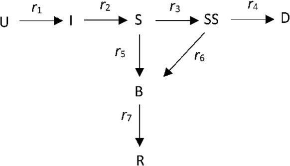
Mechanism of the COVID-19 model. U = uninfected, I = infected, S = sick, SS = seriously sick, D = dead, B = better, R = recovered; r1, etc., are rates of transition from one state to another (people per day)
The rate r1, expressing the number of healthy, nonimmune people that are infected per day, is calculated based on the following assumptions:
People in the categories I, S, SS, and B can infect healthy people, each with a different rate.
The infection rate is proportional to the fraction of people that are uninfected.
Based on these assumptions, the infection rate r1 is calculated as follows:
| 1 |
where I is the number of people in category I, etc. P is the number of people comprising the total population. k11, k12, k13, and k14 are rate constants (day−1). This equation is an extension of the infection rate in the SIR model (r = k I U/P). It assumes that the overall infection rate is the result of four parallel infection processes: infection by incubating people I (rate k11 I U/P), sick people S (rate k12 S U/P), seriously sick people SS (rate k13 SS U/P), and recovering people B (rate k14 B U/P). Each infection process has a rate proportional to the number of people in the category (I, S, …) and proportional to the fraction of uninfected people in the population (U/P).
Equation (1) assumes that the disease is homogeneously distributed across the region, and that there is no geographical variation of k11, k12, k13, and k14. Violations of this assumption may lead to inaccuracies, particularly in the late stages of the disease, when U/P significantly deviates from 1. The model is not recommended in federal countries such as the USA, where each state may adopt a different strategy to mitigate the virus. In federal countries, each state should be modeled separately.
Preliminary data fitting, as well as comparison with clinical virus shedding data indicates that k14 = 0. However, it is kept in the model for the sake of completeness.
Next, it is assumed that all other transitions are first-order processes with rate constants k2, k3, etc., with rate constants expressed in day−1. Hence:
| 2 |
| 3 |
| 4 |
| 5 |
| 6 |
| 7 |
Applying these rates to the mechanism in Fig. 1, the dynamics of the COVID-19 pandemic can be modeled with the following differential equations:
| 8 |
| 9 |
| 10 |
| 11 |
| 12 |
| 13 |
| 14 |
where t is the time in days.
The value of P is set at 100 million people in the hypothetical simulations below and set equal to the actual size of the population when specific countries are modeled. Initial conditions are given in the implementation sections. The kinetic parameters are given in the next section, with exception of the infection rate k11, which can only be determined by model fits to actual data.
The main output of the model is D (number of deaths), but the numbers of people in various stages of infection (I, S, SS, and B) is followed as well.
Parameterization
To reduce the number of adjustable parameters, the following assumptions are made:
| 15 |
| 16 |
| 17 |
As a justification for this choice of variables, it is assumed that most people will self-isolate upon experiencing symptoms, reducing the infection rate by half, whereas seriously sick people will be in bed or in the hospital, further reducing their physical or social contact with others.
The remaining parameters are shown in Table 1.
Table 1.
Parameters of the COVID-19 model
| Parameter (U) | Value |
|---|---|
| k11 (day−1) | variable |
| k2 (day−1) | ln 2/5.1 |
| k3 (day−1) | k5/9 |
| k4 (day−1) | k6 × 15/85 |
| k5 (day−1) | ln 2/3.5 |
| k6 (day−1) | ln 2/10 |
| k7 (day−1) | ln 2/10 |
k11 was determined by trial and error. In the exploratory stage, a worldwide average value of k11 was estimated by comparing the doubling rate of the total predicted number of cases of the disease by the observed number of cases. As mentioned in the Introduction, the number of cases doubled every four days. In a second, diagnostic stage, a country-specific value of k11 was obtained by fitting the cumulative number of deaths versus time to the reported data.
The value of k2 is based on the observation that the median incubation time of COVID-19 is 5.1 days [14].
The ratio k5/k3 (9) is based on the assumption that 10% of the infected become seriously sick, whereas 90% get better without developing serious symptoms. This is less than the observed proportion of roughly 80/20. The reason for the lower proportion assumed here is because many infected with mild symptoms remain undiagnosed, leading to an underreporting of mild cases. Seriously sick is defined here as needing hospitalization, regardless of whether actual hospitalization occurs.
The ratio k6/k4 is based on the assumption that 15% of hospitalized COVID-19 patient do not survive. This leads to a case mortality rate of 1.5%. This number is deliberately kept below the values reported in the Introduction because of underreporting of mild cases.
The values of k5 and k7 are based on the assumption that the median duration of the disease is 3.5 days in the “sick” stage, followed by 10 days in the “better” stage. In other words, it is assumed that people developing mild symptoms recover in about two weeks as a median value.
The value of k6 is based on the assumption that the median seriously sick patient remains in this state for 10 days. Because there is a second pathway (dying), the actual median is less, 8.5 days. This is consistent with a mean duration of 12.26 days. After adding the 3.5 days in the sick stage, a median of 12 days is obtained, somewhat shorter than clinical observations (22.0 days for discharge; 18.5 days for death [4]). However, adding the median duration of the “better” stage leads to a median of 22 days, identical with the median observed time from symptom onset to discharge time. Adding the incubation time to the sick and seriously sick conditions, a total of 17–18 days of virus shedding as a median time is obtained, close to the observed median of 20.0 days [4].
Implementation: exploratory stage
The model was implemented in Matlab. The code is given in Online Resource 1. The differential equations were integrated numerically with the fourth–fifth-order Runge–Kutta–Fehlberg algorithm (function ode45 in Matlab). The following data and initial conditions were used:
Data:
P = 100 million
Initial conditions (time = 0):
I = 100
S = 10
SS = 1
D = 0
B = 0
R = 0
U = P − I − S − SS − D − B − R
At time zero, a total of 111 infected people are assumed among a population of 100 million. This is an arbitrary choice of initial condition. As long as the initial numbers are orders of magnitude smaller than the peak values, the exact values only affect the timing of the dynamics of disease progression, not the dynamics itself. In this early phase, it can be assumed that the number of known infections will be on the order of 10 or less. In other words, we are starting the simulation very early on. The doubling time is calculated from the total number of people in all infected stages on day 29 and day 30 with the equation:
| 18 |
where Cn is an estimate of the number of known or reported “cases” on day n. The number of known cases is assumed to be 5% of infected, a third of sick, 90% of seriously sick, 12% of recovering, 12% of recovered, and 90% of deceased patients. The calculated doubling time is not sensitive to the choice of these fractions.
To calculate the value of R0 (the number of people infected by the average carrier of the virus), a separate simulation was run with a single infected case, where the number of newly infected is calculated over time.
To model non-pharmaceutical interventions (NPI), an effectiveness E is defined such that:
| 19 |
The effectiveness E is not generally a constant that is established instantaneously when NPI are imposed. In practice, it will typically take a few days to completely roll out a mitigation strategy. Some people may anticipate the measure in their behavior before the actual measure takes effect.
To operationalize this, a smooth function for k11 was used to model the implementation of the NPI over the days following the NPI decision:
| 20 |
where k11,0 is the infection rate in the absence of interventions, ti is the day after the time of the intervention decision, and erf stands for the error function. Equation (20) uses the property erf(–x) = –erf(x). To illustrate this, Fig. 2 shows the value of k11 versus time for an intervention decision on day 30, where k11,0 = 0.4 and E = 0.8. As the figure illustrates, Eq. (20) has the desired properties: a gradual decrease in the infection rate over a couple of days, with a slight decrease anticipating the actual measure.
Fig. 2.
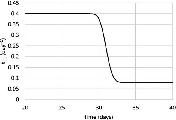
k11 versus time for a non-pharmaceutical intervention on day 30. k11,0 = 0.4, E = 0.8
Implementation: diagnostic phase
In the diagnostic phase, time zero is set to February 1, 2020. The initial numbers of I (100), S (10), and SS (1) are multiplied by a correction factor, which provides a second adjustable variable in addition to k11. k11 and the correction factor are adjusted by trial and error until the predicted cumulative deaths predicted as a function of time before the NPI closely matches the reported number of deaths. The timing of the NPI (ti) is chosen as the date of the main government decision to impose NPI, typically the date when the government imposes a lockdown. When there is a clear sequence of government measures with increased severity, multiple dates are chosen, each with an incremental effectiveness. In that case, k11 is calculated as follows:
| 21 |
where n is the number of NPIs considered in the model, E1, E2, … is the effectiveness of the first, second, … intervention, and t1, t2, … is the date of the first, second, … intervention. Each effectiveness is incremental and chosen with respect to k11,0, i.e., the overall effectiveness after all measures have been taken is the sum of the Ej values. This sum cannot exceed one. A reopening of the economy can be modeled by means of an intervention with a negative incremental effectiveness.
The efficiency or efficiencies of the NPI were determined by trial and error, by comparing modeled deaths with reported deaths. The number of NPIs is chosen as small as possible, to minimize overfitting.
The choice of fitting number of deaths rather than number of cases has a number of advantages. First, the precise date of deaths is generally known, whereas there are generally no data on the exact date of infection. Second, the number of reported deaths is less sensitive to undercounting due to asymptomatic or weakly symptomatic cases. Third, number of cases, even as a relative measure, is sensitive to changes in testing policies, shortage of test kits, and lag times between taking the test and obtaining the test results. Reported deaths are likely less sensitive to such issues. There are disadvantages of fitting the model to death data as well. First, the death numbers respond more slowly to changing behavior or changing policies. Second, death numbers are sensitive to improving treatment procedures.
In some cases, spikes in k11 are considered to account for events (e.g., festivals, etc.) where large numbers of people are gathered or where large numbers of new infections can be expected over a short time. In that case, a Gaussian curve centered around the time of the event with a standard deviation of 0.5 days is added to the calculation of k11:
| 22 |
Results
Doubling times, infection rates, reproduction numbers
First, the doubling time of the pandemic is calculated for different values of the infection rate k11. As mentioned in the Introduction, the worldwide doubling time of COVID-19 outside China was 4 days in the latter half of February and the first half of March 2020. This doubling time was found to correspond with k11 = 0.261 day−1. This value was used as the default in further simulations, unless specified otherwise.
In Europe and North America, doubling times were significantly shorter during that time. For instance, in Italy, the reported number of COVID-19 cases grew approximately exponentially from 150 on February 23 to 10,149 on March 10 (16 days later) (https://www.worldometers.info/coronavirus/country/italy/). An exponential fit to the data leads to a doubling time of 2.66 days (R2 = 0.9841). This is consistent with k11 = 0.344 day−1. Most of the Western world experienced similar growth rates during the same time.
The R0 value was calculated as a function of k11. The relationship between R0 and k11 follows a perfect linear relationship as follows:
| 19 |
where a = 10.0388 days. The value of a depends on the other kinetic parameters as well, but because they were either kept constant, or kept proportional to k11, the value of a can be considered as a constant in the current study.
The R0 value reaches 1 when k11 = 0.0996 day−1, only 38.1% of the global average k11 value in late February to early March 2020, and 29.0% of the value in Italy during that time. As a result, the model-based estimate for R0 in late February to early March is 2.62 worldwide outside China, and 3.45 in Italy and most of the Western world. These are just estimations based on the assumption that the proportion of cases reported remains constant over time.
Scenarios: average, fast, slow
In this section, a number of scenarios will be run to assess the number of infected and the number of deaths as a function of time, for a population of 100 million, starting with 111 infected (100 incubating, 10 sick, and 1 seriously sick) at time 0.
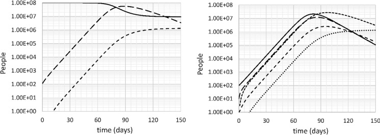
Figures 3 shows the evolution of the epidemic in the base case (doubling time = 4 days, k11 = 0.261 day−1, R0 = 2.62), without intervention. The first deaths are predicted around day 12, when about 1200 people are infected. The number of people showing symptoms at this time is around 460 (250 mild, 20 serious, 190 recovering). This early in the epidemic, it is likely that testing is not yet fully deployed, and the number of reported cases is likely to be on the order of 200 or less.
Fig. 3.
Left: uninfected (U: solid), all infected (I + S + SS + B: long dash) and deceased (D: short dash) people versus time. Right: Incubating (I: solid), sick (S: long dash), seriously sick (SS: short dash), recovering (B: very short dash) and deceased (D: dotted) people versus time. Base case, no intervention, doubling time 4 days
After 1 month, the model predicts 30–35 deaths and a total of about 27,000 infected. Of these, about 16,000 show no symptoms, 5000 show mild symptoms, 500 severe symptoms, and 5000 are recovering. At this point, the official case count is probably a few thousands. Around this time or up to two weeks later, most governments started taking serious precautions to limit the spread of the virus.
After two months without intervention, there are 4.5 million infections and over 6000 deaths. As a rule of thumb, there is one death per 750 cases in the expansion phase of the disease when the doubling time is 4 days. 2.7 million people are in the incubation phase, and 85,000 people are seriously sick.
The peak of seriously sick people is reached on day 95, when over 2.5 million people are seriously sick and over half a million people have died.
After 150 days, the disease is declining but is still overwhelming the health care system, with about 180,000 people seriously sick. The model predicts 1.33 million deaths at this time, 1.33% of the population. Given the severe lack of care that would occur, the death toll could be underestimated by as much as a factor 2 or 3. About 91.6 million people get infected overall, significantly more than the expected number from “herd immunity” (61.8 million). This is because the disease expands so rapidly that it overshoots and continues to infect people as it winds down past the 62 million mark. This simulation clearly shows that herd immunity is only effective when people are vaccinated before the spread of the disease.
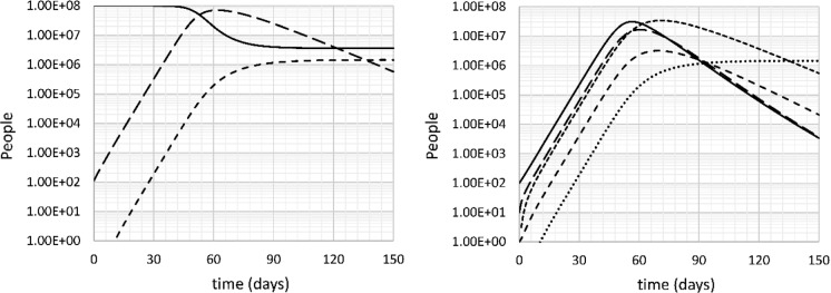
Next, the simulation was repeated for a “fast” scenario where the doubling time is the same as in Italy in late February to early March, 2.66 days (k11 = 0.344 day−1, R0 = 3.45). The results are shown in Fig. 4. The main difference with the base case is that the disease spreads faster and peaks sooner. At its peak, 3.2 million people are seriously sick, on day 70. The death burden after 150 days is 1.44 million, or 1.44% of the population. At this time, the disease has affected 96.4 million people, 96.4% of the population. Again, this is massively above the number expected from herd immunity (71.0 million people).
Fig. 4.
Left: uninfected (U: solid), all infected (I + S + SS + B: long dash) and deceased (D: short dash) people versus time. Right: Incubating (I: solid), sick (S: long dash), seriously sick (SS: short dash), recovering (B: very short dash) and deceased (D: dotted) people versus time. Fast case, no intervention, doubling time 2.66 days
During the initial spread of the disease, there is one death every 1800–2000 cases, indicating that the epidemic may be underestimated even more when it spreads rapidly. This ratio explains why the case mortality rate of COVID-19 is sometimes incorrectly speculated to be on the order of 0.1% (https://www.forbes.com/sites/carlieporterfield/2020/04/21/scientists-widely-criticize-studies-that-claim-coronavirus-death-rate-could-be-far-lower-than-believed/#31cde7711517: accessed April 22, 2020).
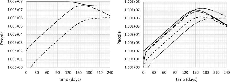
The next scenario is a “slow” scenario. It represents a containment strategy that is popularized as “flattening the curve.” For the purpose of this paper, a containment strategy is defined as a strategy to significantly reduce the infection rate in order to slow down the spread of the disease in an attempt to avoid overburdening the health care system, but with no attempts to eradicate the disease, i.e., the R0 remains significantly above 1. The simulation is run with an infection rate k11 = 0.18 day−1 (doubling time 7.65 days, R0 = 1.81). The result is shown in Fig. 5.
Fig. 5.
Left: uninfected (U: solid), all infected (I + S + SS + B: long dash) and deceased (D: short dash) people versus time. Right: Incubating (I: solid), sick (S: long dash), seriously sick (SS: short dash), recovering (B: very short dash) and deceased (D: dotted) people versus time. Slow case, no intervention, doubling time 7.65 days
The peak in the number of seriously sick people is significantly delayed, to day 185, but the number of patients still far exceeds the capacity of any health care system, with 1.4 million seriously sick, half the number of the base case. The death burden in the “flattening the curve” strategy is slightly over 1 million, still over two-thirds of the fast scenario. The total number of people that get infected in a 240-day time span is 73.3 million, again markedly more than the number expected from herd immunity considerations (44.7 million).
Clearly, containment as defined here is an inadequate strategy for fighting the COVID-19 pandemic.
Scenarios: social distancing intervention for elimination of the virus
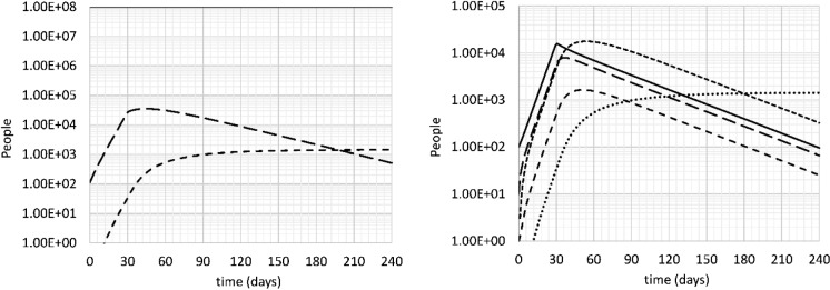
Next, starting from the base case, it is assumed that drastic social distancing measures are taken on day 30 that reduce R0 to below 1. This is a strategy of elimination, as opposed to the containment strategy discussed in the previous section. It is assumed that the value of k11 is reduced by 70% (i.e., from 0.261 to 0.0783 day−1, i.e., R0 decreases from 2.62 to 0.786). The result is shown in Fig. 6. A 70% effective social distancing intervention with a starting value of k11 = 0.261 day−1, i.e., with respect to the world average, is equivalent with a 77% effective intervention with a starting value of k11 = 0.344 day−1, i.e., with respect to the situation in Italy and most of the Western world. In other words, in much of the Western world, the results shown in Fig. 6 reflect a social distancing initiative that is 77% effective, not 70%.
Fig. 6.
Left: uninfected (solid), all infected (long dash) and deceased (short dash) people versus time. Right: Incubating (solid), sick (long dash), seriously sick (short dash), recovering (very short dash) and deceased (dotted) people versus time. Base case, doubling time 4 days, intervention on day 30 with 70% effectiveness
There is a marked decline in the number of infected in this scenario. After 240 days, the number of people who died of COVID-19 is 1420, about three orders of magnitude less than the previous scenarios. Still, this number is 42 times the number people who had died at the onset of the intervention (34).
The number of seriously sick people peaks at a value of 1642 on day 51, again about three orders of magnitude less than in the preceding scenarios.
What is clear from this scenario is that the decline of the epidemic is much slower than its growth. This has important repercussions for any public health policy aiming to save lives. Even 7 months into the intervention, the number of infected is comparable to the number of infected two and a half weeks before the intervention. Terminating the intervention would immediately relaunch the epidemic. The reproductive number must be maintained below 1 until the population can be vaccinated on a large scale.
Scenarios: the death burden of inaction
In this section, the number of deaths will be evaluated as a function of time and effectiveness of the social distancing intervention. The starting point is the base case, with a doubling time of 4 days (k11 = 0.261 day−1, R0 = 2.62).
First, the effect of effectiveness of the social distancing intervention is calculated. It is assumed that the intervention starts on day 30 with an effectiveness ranging from 50 to 80%. Figure 7 shows the number of deaths after 60, 150, and 300 days.
Fig. 7.
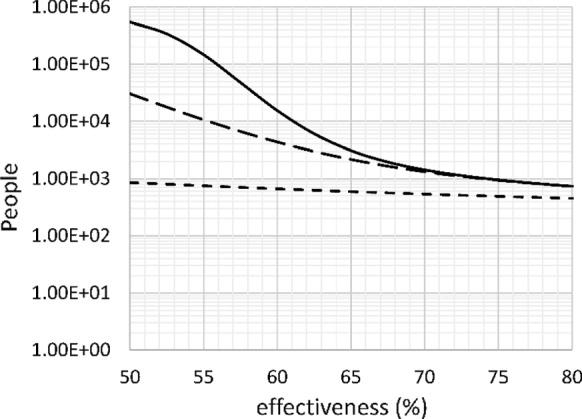
Number of deaths after 60 days (short dash), 150 days (long dash) and 300 days (solid) versus effectiveness of intervention. Base case, doubling time 4 days, intervention on day 30
After 60 days, i.e., 30 days after the start of the intervention, the effect of effectiveness of intervention on mortality is very limited. This is concerning because to observers it appears that the interventions are not working. However, over a 150-day time span, a 5% decrease in efficiency can triple the mortality. Over a 300-day time span, a 1% decrease in the efficiency (e.g., from 62% to 61%) can cause a 50% increase in mortality. This explains why some Asian countries treat seemingly trivial violations of the social distancing rules as felonies.
The value of R0 equals 1 at 61.8% efficiency in this case. The importance of keeping R0 below 1 is immediately obvious from Fig. 7. When the initial value of k11 is 0.344 day−1, an efficiency of 71.0% is needed to lower R0 to 1. This should be the minimum target efficiency of social distancing in Europe and North America.
Next, the effect of timing of introduction of a social distancing intervention on the mortality over 60 days, 150 days, and 300 days is calculated. The results are shown in Fig. 8. Probably not surprisingly, the number of deaths doubles with every 4-day delay of the introduction of social distancing. This is an important point, because the number of deaths may seem small at the time of introduction (e.g., from 34 on day 30 to 68 on day 34), the number of deaths after 300 days increases from 1429 to 2845 as a result of this delay. Every additional death at the time of intervention represents 42 additional deaths over a 300-day time span.
Fig. 8.
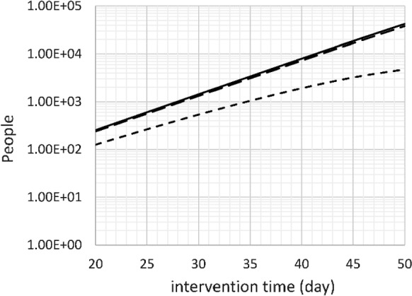
Number of deaths after 60 days (short dash), 150 days (long dash) and 300 days (solid) versus time of intervention. Base case, doubling time 4 days, intervention effectiveness 70%
Diagnostic modeling: NPI phase
In this section, modeled deaths versus time will be compared with reported deaths in three countries: Italy, France, and Iran. These countries were chosen because they were hit relatively early so there is more data, the death toll for these countries is relatively high, and they represent three distinct cases. For each country, an analysis was made in early April, and again in late April. The death rate data used to calibrate the models, as well as the modeling results, are given in Excel format in Online Resource 2. The early analyses were presented on YouTube to document and time-stamp the projections (see https://www.youtube.com/watch?v=7Y9fwus0fvQ for Italy, https://www.youtube.com/watch?v=MT4wjniICLY for France, and https://www.youtube.com/watch?v=z1DMM68HHB8 for Iran). The results of the two analyses are compared. The adjustable parameter values obtained in each analysis is compared in Table 2. In all but the Italian case, only one NPI event was needed to explain the entire data set. As a result, E2 and E3 were set equal to 0 in the case of France and Iran. In both cases, adding more interventions could have been added to the model, but the quality of fit between the model and the data indicates that this was not necessary.
Table 2.
Adjustable parameters of the COVID-19 spread in Italy, France, and Iran, obtained in early April and late April
| Country | Italy | Italy | France | France | Iran | Iran |
|---|---|---|---|---|---|---|
| Analysis date | April 3 | April 21 | April 9 | April 21 | April 5 | April 21 |
| k11,0 (day−1) | 0.378 | 0.40 | 0.323 | 0.323 | 0.32 | 0.34 |
| Correction | 0.136 | 0.08 | 0.049 | 0.049 | 0.518 | 0.296 |
| t1 | March 9 | March 2 | March 24 | March 24 | March 5 | March 5 |
| E1 | 0.794 | 0.224 | 0.87 | 0.89 | 0.73 | 0.8 |
| t2 | – | March 9 | – | – | – | – |
| E2 | – | 0.46 | – | – | – | – |
| t3 | – | March 21 | – | – | – | – |
| E3 | – | 0.226 | – | – | – | – |
| kspike | – | – | – | – | – | 0.6 |
| tspike | – | – | – | – | – | March 20 |
| Population | 60.5 × 10⁶ | 60.5 × 10⁶ | 65.2 × 10⁶ | 65.2 × 10⁶ | 83.7 × 10⁶ | 83.7 × 10⁶ |
| Projected deaths | 47,620 | 31,323 | 35,156 | 32,499 | 13,676 | 8061 |
Note that tj is the day after the NPI decision, whereas tspike is the day of the event leading to the spike
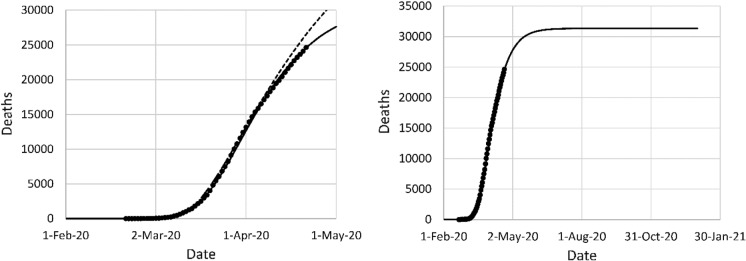
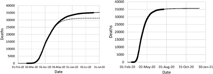
The model fit to the data in Italy is shown in Fig. 9. The initial fit was based on a single NPI on March 8, the day a national lockdown was declared. This fit provided a poor prediction of the data after April 3, due to the complexity of the situation. The epidemic started in the region of Lombardy, in the North of Italy, and spread to the rest of the country. The second fit required three NPI phases and still showed some lack of fit. The total mortality projection declined from about 47,000 based on the original fit to about 31,000 based on the second fit.
Fig. 9.
Left: original model fit to reported deaths in Italy up to April 3 (long dash) and projection after April 3 (short dash), second data fit (solid); (right) mortality projection based on second fit. Circles: cumulative reported deaths
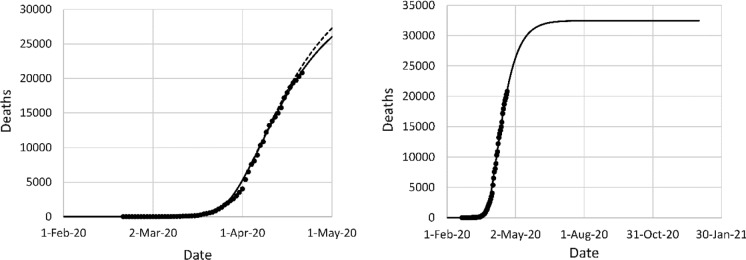
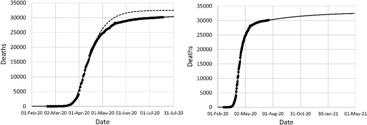
Figure 10 shows the data for France, with the model fits. The overall efficiency of the NPI is similar to the Italian case, but in France, the lockdown was more sudden in France and occurred at a later date. The projections of the original model fit are more accurate in the case of France in comparison with Italy, because a single lockdown decision explains the entire data set. The lack of fit in Fig. 10 is mainly due to late reporting of some cases, particularly deaths occurring in retirement homes. The mortality projection was 35,156 in the first data fit, and 32,449 in the second data fit. On April 9, the last data point of the first fit, the reported mortality in France was 12,210.
Fig. 10.
Left: original model fit to reported deaths in France up to April 9 (long dash) and projection after April 9 (short dash), second data fit (solid); (right) mortality projection based on second fit. Circles: cumulative reported deaths
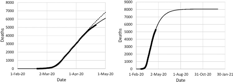
The data for Iran are shown in Fig. 11. Prediction of the epidemic in Iran was complicated by the Iranian New Year, which occurred on March 20. The quality of fit improved upon adding a spike in the infection rate on that day. Because the spike masked the effectiveness of the NPI in Iran, the mortality projection from the first model fit was a serious overestimate (over 13,000 deaths) in comparison with the second fit (around 8000 deaths). The relatively low mortality in Iran is thanks to the earlier intervention. As long as the reproduction number of the disease is brought below 1, an early timing of the intervention is more important than the effectiveness.
Fig. 11.
Left: original model fit to reported deaths in Iran up to April 5 (long dash) and projection after April 5 (short dash), second data fit (solid); (right) mortality projection based on second fit. Circles: cumulative reported deaths
Preliminary mortality rate estimation: Netherlands
On April 16, 2020, Reuters reported a study of 10,000 blood donations in The Netherlands, indicating that 3% of the samples contained antibodies against SARS-CoV-2 (https://www.reuters.com/article/us-health-coronavirus-netherlands-study/dutch-study-suggests-3-of-population-may-have-coronavirus-antibodies-idUSKCN21Y102). The study is non-peer-reviewed and no methodological details were given, so this analysis is preliminary at best. Assuming that the test results are correct and the sample set is representative of the population in The Netherlands, this leads to an estimated 510,000 coronavirus positive people of a population of 17 million. The model was fitted to mortality data in The Netherlands as shown in Online Resource 3. The obtained values were k11 = 0.34, interventions on March 15 and March 23 with effectiveness 0.34 and 0.58, respectively, and a correction of 0.00118. This leads to a long-term projected mortality of 5800. On April 8, a week before the report, the number of coronavirus positive cases in The Netherlands is predicted at 360,000 by the model, of the same order of magnitude as the estimate from the blood donation samples. A refit indicates that the model would predict a case number of 510,000 if a case mortality rate of 1.06% is assumed.
This case mortality rate estimation does not account for inaccuracies in the immunological testing. Assuming a test specificity of 99% (i.e., a false positive rate of 1%), the real number of cases would be 343,000, leading to a case mortality rate of 1.57%. If a test specificity of 98% is assumed, the real number of cases would be 173,000, and the case mortality rate would be as high as 3.12%. It follows that the data impose a lower limit of the case mortality on the order of 1% and will be higher unless the test used is exceedingly specific.
Diagnostic modeling: reopening phase
The modeling of coronavirus deaths in Iran, Italy, and France, including reopening data, is based on data given in Online Resource 4. Whereas the data in Sect. 3.5 were analyzed before submission of the original manuscript in late April, this section is based on a data analysis carried out in July, during preparation of the revised manuscript. None of the numbers in Sect. 3.5 were altered during the revision.
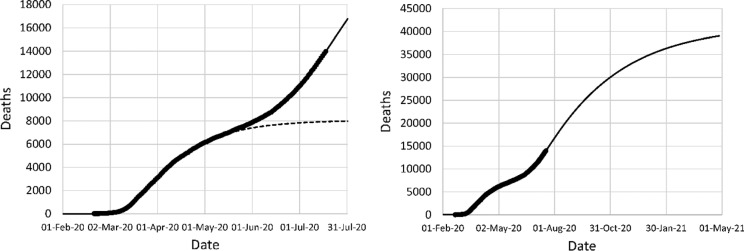
In some countries, the reopening of the economy after a successful NPI phase has led to a renewed spiking of coronavirus cases, sometimes leading to a resurgence of coronavirus deaths. An example is Iran, where the economy was gradually reopened in late April and early May. By the end of June, the Iranian government introduced the requirement to wear face masks in public spaces.
The model was fitted to coronavirus deaths up to July 18. The parameters are shown in Table 3. An intervention with effectiveness − 18.5% on May 1 was introduced to represent the reopening. For a good fit of the model, it was necessary to add an additional intervention on June 1, with effectiveness 1.5%. Late June, the Iranian Government mandated the wearing of facemasks in public spaces. An intervention with effectiveness 9.25% (i.e., a reduction in k11 by 25%) was introduced in the model on July 1 to account for this. The result is shown in Fig. 12. A good fit between the model and the data is observed. The model predicts nearly 40,000 deaths by the spring of 2021, almost five times the prediction made on April 21. Clearly, a reopening can have a devastating effect if it pushes the reproduction rate of the virus above 1. If the recent decrease in the infection rate modeled by E4 = 0.0925 is indeed caused by the introduction of facemasks, then the impact of this measure in terms of lives saved can be calculated by setting E4 = 0 and comparing the results. This calculation indicates that the long-term death toll with E4 = 0 would be 463,000, indicating that this measure may save over 420,000 lives. Projections based on this type of calculations would allow governments to make rational decisions about reopening their economy.
Table 3.
Adjustable parameters of the COVID-19 spread in Italy, France, and Iran, obtained in late April and mid-July
| Country | Italy | Italy | France | France | Iran | Iran |
|---|---|---|---|---|---|---|
| Analysis date | April 21 | July 18 | April 21 | July 18 | April 21 | July 18 |
| k11,0 (day−1) | 0.40 | 0.40 | 0.323 | 0.323 | 0.34 | 0.34 |
| Correction | 0.08 | 0.08 | 0.049 | 0.049 | 0.296 | 0.296 |
| t1 | March 2 | March 2 | March 24 | March 24 | March 5 | March 5 |
| E1 | 0.224 | 0.224 | 0.89 | 0.92 | 0.8 | 0.8 |
| t2 | March 9 | March 9 | – | May 12 | – | May 1 |
| E2 | 0.46 | 0.46 | – | –0.1 | – | –0.185 |
| t3 | March 21 | March 21 | – | June 1 | – | June 1 |
| E3 | 0.226 | 0.226 | – | –0.12 | – | 0.015 |
| t4 | March 31 | July 1 | ||||
| E4 | –0.05 | 0.0925* | ||||
| t5 | May 18 | |||||
| E5 | –0.05 | |||||
| kspike | – | – | – | – | 0.6 | 0.6 |
| tspike | – | – | – | – | March 20 | March 20 |
| Population | 60.5 × 10⁶ | 60.5 × 10⁶ | 65.2 × 10⁶ | 65.2 × 10⁶ | 83.7 × 10⁶ | 83.7 × 10⁶ |
| Projected deaths | 31,323 | 35,656 | 32,499 | 32,476 | 8061 | 39,022 |
Note that tj is the day after the NPI decision, whereas tspike is the day of the event leading to the spike
*Corresponding with a reduction in k11 of 25% at the time of implementation
Fig. 12.
Left: fit to reported deaths in Iran up to April 21 (long dash) and projection after April 21 (short dash), post-reopening data fit (solid); (right) mortality projection based on second fit. Circles: cumulative reported deaths
Italy started reopening around May 18. This was modeled with a negative efficiency of −5% starting on that date. To obtain a good fit with the reported deaths, an additional negative efficiency of −5% had to be assumed, starting on March 31. The long-term death projection increases from slightly over 31,000 to slightly over 35,000. The model fit is shown in Fig. 13. Clearly, the previous model fit underestimated the ultimate number of deaths. The reopening only affects deaths after early to mid-June and has only a minor effect. For now, it can be concluded that Italy’s reopening is successful.
Fig. 13.
Left: fit to reported deaths in Italy up to April 21 (long dash) and projection after April 21 (short dash), post-reopening data fit (solid); (right) mortality projection based on second fit. Circles: cumulative reported deaths
To obtain a good fit with the France data, the efficiency of the original NPI had to be increased further, from 89% to 92%. The reopening started around June 1, but a reversal in the death trend occurred too soon to be explained by the reopening alone. For that reason, an additional NPI on May 12 with effectiveness − 10% was assumed, along with an NPI on June 1 with effectiveness − 12%. The fit of the model with the data is shown in Fig. 14. As with Italy, the progression of deaths is somewhat underestimated in the April 21 projection, but the underestimation is undone by the reopening, which adds several thousands to the death toll. The calculations indicate that the reproduction number in France as of mid-July is dangerously close to 1, and further initiatives to reopen the economy should be combined with mitigating measures.
Fig. 14.
Left: fit to reported deaths in France up to April 21 (long dash) and projection after April 21 (short dash), post-reopening data fit (solid); (right) mortality projection based on second fit. Circles: cumulative reported deaths
To confirm the model’s ability to describe the COVID-19 epidemic in a range of countries, additional analyses were conducted on data of Spain and Germany. The data and model fits are shown in Online Resource 5. The parameter values, as well as a brief discussion, are given in Online Resource 6.
Discussion
The worldwide average R0 value of COVID-19 outside China is estimated at 2.82 for the late February—early March 2020 period, based on a doubling time of 4 days for the number of cases, whereas the value was around 3.83 at the same time in the Western world, based on a doubling time of 2.66 days. For the countries investigated, values ranging from 3.23 to 4.02 were found. This is significantly higher than regular influenza viruses, which have a mean R0 of 1.3 [15]. As a result, experience with flu is a poor guide for predicting the course of the COVID-19 epidemic. For instance, flu viruses are seasonal because their R0 tend to drop below 1 over the summer months, but COVID-19 is too contagious to display a similar seasonality without strict NPI.
The case mortality rate assumed in the model 1.5% was assumed to be constant. In practice, the value is strongly age and gender specific. The value is also expected to increase in cases where the hospital system is overwhelmed. These factors were not accounted for and may lead to deviations between modeled and reported deaths. The assumed mortality is lower than current estimated values. The main sources of error in estimated values are underreporting of cases due to lack of testing, which leads to overestimation, and the time lag between illness and death, which leads to underestimation. The analysis of blood sample data from The Netherlands tentatively indicates a value of 1% or more, depending on the specificity of the testing, indicating that the number used here, as well as the current estimates, are in the correct range.
The model predicts that there is 1 death per 750 cases during the growth phase of the epidemic when the doubling time is 4 days, and 1 death per nearly 2000 cases when the doubling time is 2.66 days. With approximately 50,000 deaths as of April 1, when the growth rate of the epidemic started to decline, this means that the number of infected was probably on the order of 40 million people around that time. Assuming a death rate of 1.5%, a lower limit of 600,000 deaths can be expected worldwide, even if no new infections occur.
Irrespective of the variables used, model predictions indicate that COVID-19 will affect vastly more people than expected from “herd immunity” considerations. This is because there is a huge number of infected people at the time of onset of herd immunity, enough to infect most of the remaining uninfected people before the epidemic spirals down. It follows that public health strategies based on herd immunity are extremely misguided and extremely deadly. Herd immunity is only effective when the population is vaccinated before the onset of the disease.
Likewise, a public health strategy based on containment (“flattening the curve”) without diminishing R0 below 1 is inadequate and extremely deadly, with an expected mortality rate of about 1% based on the entire population even with the unrealistic assumption that the healthcare system can handle the number of patients. Only measures that bring the reproduction number below 1 significantly reduce number of deaths.
Once a country takes decisive action to reduce R0 below 1, the mortality still increases by about a factor 42 before the disease is stopped. Based on that number, the estimate of 600,000 deaths is probably vastly underestimated.
The mortality of COVID-19 after intervention is very sensitive to the effectiveness of the intervention, particularly when the reproductive number is close to 1. Minor gaps in the social distancing policy (e.g., closing bars but allowing private parties), or a small fraction of the population violating the policy can have disastrous effects on mortality rates.
Simulations of the effect of reopening on the epidemic in Italy, France, and Iran were carried out. Reopenings were successfully modeled by adding additional NPIs with negative effectiveness (typically − 10 to − 20%). Hence, the model can be used to evaluate if a country is ready for reopening, and to make projections of the effect of reopening on the number of deaths.
Software
The software of the model consists of two MATLAB files, main_ND.m and f_ND.m. The file main_ND.m is the control file that should be run. The file f_ND.m defines the differential equations. The model can be run on MATLAB, or on its open-source equivalent GNU Octave (https://www.gnu.org/software/octave). The source code is shown in the supporting document, Online Resource 1 and can be obtained from the author by e-mail.
Two additional files are included for the calculation of R0: main_ND_R0.m and f_ND_R0.m.
For terms of use: see source code.
Conclusions
Calculations with an epidemiological model developed to describe the spread of the COVID-19 pandemic indicates that highly successful social distancing measures are needed to keep the mortality of the pandemic below 1% of the population. With successful social distancing implemented early, the death burden can be reduced by up to three orders of magnitude.
The model can be applied to specific countries and used to make projections of future death rates. Robust predictions can be made approximately 1 month after the onset of social distancing, provided the initiative is swift and decisive.
Based on a (non-peer reviewed) study of blood donation samples in The Netherlands, a lower limit on the case mortality rate of COVID-19 has been preliminarily set to 1%.
Electronic supplementary material
Below is the link to the electronic supplementary material.
Funding
None.
Availability of data and materials
Data of Figures 9–14, as well as additional data and figures for Spain and Germany are included in supporting documents.
Code availability
Code is included in supporting document.
Compliance with ethical standards
Conflict of interest
The author declares that they have no conflict of interest.
Footnotes
Publisher's Note
Springer Nature remains neutral with regard to jurisdictional claims in published maps and institutional affiliations.
References
- 1.Xu Z, Shi L, Wang Y, Zhang J, Huang L, Zhang C, Liu S, Zhao P, Liu H, Zhu L, Tai Y, Bai C, Gao T, Song J, Xia P, Dong J, Zhao J, Wang FS. Pathological findings of COVID-19 associated with acute respiratory distress syndrome. Lancet Respir. Med. 2020;8:420–422. doi: 10.1016/S2213-2600(20)30076-X. [DOI] [PMC free article] [PubMed] [Google Scholar]
- 2.Mehta P, McAuley DF, Brown M, Sanchez E, Tattersall RS, Manson J. COVID-19: consider cytokine storm syndromes and immunosuppression. Lancet. 2020;395:1033–1034. doi: 10.1016/S0140-6736(20)30628-0. [DOI] [PMC free article] [PubMed] [Google Scholar]
- 3.Zheng YY, Ma YT, Zhang JY, Xie X. COVID-19 and the cardiovascular system. Nat. Rev. Cardiol. 2020;17:259–260. doi: 10.1038/s41569-020-0360-5. [DOI] [PMC free article] [PubMed] [Google Scholar]
- 4.Zhou F, Yu T, Du R, Fan G, Liu Y, Liu Z, Xiang J, Wang Y, Song B, Gu X, Guan L, Wei Y, Li H, Wu X, Xu J, Tu S, Zhang Y, Chen H, Cao B. Clinical course and risk factors for mortality of adult inpatients with COVID-19 in Wuhan, China: a retrospective cohort study. Lancet. 2020;395:1054–1062. doi: 10.1016/S0140-6736(20)30566-3. [DOI] [PMC free article] [PubMed] [Google Scholar]
- 5.Feng Z, Li Q, Zhang Y, Wu Z, Dong X, Ma H, Yin D, Lyu K, Wang D, Zhou L, Ren R, Li C, Wang Y, Ni D, Zjao J, Li B, Wang R, Niu Y, Wang X, Zhang L, Sun J, Liu B, Deng Z, Ma Z, Yang Y, Liu H, Shao G, Li H, Liu Y, Zhang H, Qu S, Lou W, Shan D, Hu Y, Hou L, Zhao Z, Liu J, Wang H, Pang Y, Han Y, Ma Q, Ma Y, Chen S, Li W, Yang R, Li Z, Guo Y, Liu X, Jiangtulu B, Yin Z, Xu J, Wang S, Xiao L, Xu T, Wang L, Qi X, Shi G, Tu W, Shi X, Su X, Li Z, Luo H, Ma J, McGoogan JM. The epidemiological characteristics of an outbreak of 2019 Novel Coronavirus Disease (COVID-19)—China, 2020. CCDC Wkly. 2020;2:112–122. [PMC free article] [PubMed] [Google Scholar]
- 6.Liu Y, Gayle AA, Wilder-Smith A, Rocklöv J. The reproductive number of COVID-19 is higher compared to SARS coronavirus. J. Travel Med. 2020 doi: 10.1093/jtm/taaa021. [DOI] [PMC free article] [PubMed] [Google Scholar]
- 7.van Doremalen N, Bushmaker T, Morris DH, Holbrook MG, Gamble A, Williamson BN, Tamin A, Harcourt JL, Thornburg NJ, Gerber SI, Lloyd-Smith J, de Wit E, Munster VJ. Aerosol and surface stability of SARS-CoV-2 as compared with SARS-CoV-1. N. Engl. J. Med. 2020;382:1564–1567. doi: 10.1056/NEJMc2004973. [DOI] [PMC free article] [PubMed] [Google Scholar]
- 8.Nishiura H, Linton NM, Akhmetzhanov AR. Serial interval of novel coronavirus (COVID-19) infections. Int. J. Infect. Dis. 2020;93:284–286. doi: 10.1016/j.ijid.2020.02.060. [DOI] [PMC free article] [PubMed] [Google Scholar]
- 9.Kermack WO, McKendrick AG. A contribution to the mathematical theory of epidemics. Proc. R. Soc Edinb. A. 1927;115:700–721. [Google Scholar]
- 10.Satsuma J, Willox R, Ramani A, Grammaticos B, Carstea AS. Extending the SIR epidemic model. Phys. A. 2004;336:369–375. doi: 10.1016/j.physa.2003.12.035. [DOI] [Google Scholar]
- 11.Lin Q, Zhao S, Gao D, Lou Y, Yang S, Musa SS, Wang MH, Cai Y, Wang W, Yang L, He D. A conceptual model for the coronavirus disease 2019 (COVID-19) outbreak in Wuhan, China with individual reaction and governmental action. Int. J. Infect. Dis. 2020;93:211–216. doi: 10.1016/j.ijid.2020.02.058. [DOI] [PMC free article] [PubMed] [Google Scholar]
- 12.Roosa K, Lee Y, Luo R, Kirpich A, Rothenburg R, Hyman JM, Yan P, Chowell G. Real-time forecasts of the COVID-19 epidemic in China from February 5th to February 24th, 2020. Infect. Disease Model. 2020;5:256–263. doi: 10.1016/j.idm.2020.02.002. [DOI] [PMC free article] [PubMed] [Google Scholar]
- 13.Ferguson NM, Cummings DAT, Cauchemez S, Fraser C, Riley S, Meeyai A, Iamsirithaworn S, Burke DS. Strategies for containing an emerging influenza pandemic in Southeast Asia. Nature. 2005;437:209–214. doi: 10.1038/nature04017. [DOI] [PubMed] [Google Scholar]
- 14.Lauer SA, Grantz KH, Bi Q, Jones FK, Zheng Q, Meredith HR, Azman AS, Reich NG, Lessler J. The incubation period of coronavirus disease 2019 (COVID-19) from publicly reported confirmed cases: estimation and application. Ann. Internal Med. 2020 doi: 10.7326/M20-0504. [DOI] [PMC free article] [PubMed] [Google Scholar]
- 15.Chowell G, Miller MA, Viboud C. Seasonal influenza in the United States, France, and Australia: transmission and prospects for control. Epidemiol. Infect. 2008;136:852–864. doi: 10.1017/S0950268807009144. [DOI] [PMC free article] [PubMed] [Google Scholar]
Associated Data
This section collects any data citations, data availability statements, or supplementary materials included in this article.
Supplementary Materials
Data Availability Statement
Data of Figures 9–14, as well as additional data and figures for Spain and Germany are included in supporting documents.
Code is included in supporting document.


