Improving the Speed of MRI with Artificial Intelligence

Abstract

Magnetic resonance imaging (MRI) is a leading image modality for the assessment of musculoskeletal (MSK) injuries and disorders. A significant drawback, however, is the lengthy data acquisition. This issue has motivated the development of methods to improve the speed of MRI. The field of artificial intelligence (AI) for accelerated MRI, although in its infancy, has seen tremendous progress over the past 3 years. Promising approaches include deep learning methods for reconstructing undersampled MRI data and generating high-resolution from low-resolution data. Preliminary studies show the promise of the variational network, a state-of-the-art technique, to generalize to many different anatomical regions and achieve comparable diagnostic accuracy as conventional methods. This article discusses the state-of-the-art methods, considerations for clinical applicability, followed by future perspectives for the field.

Magnetic resonance imaging (MRI), which offers high-resolution images and unparalleled soft tissue contrast, is a leading image modality for the assessment of musculoskeletal (MSK) injuries and disorders. The acquisition of MRI data is an inherently slow process due to the high sampling requirements. The long data acquisition leads to low patient throughput, patient discomfort, artifacts from patient motion, and therefore costly examinations. These drawbacks have motivated the development of methods for faster MR imaging.

Artificial intelligence (AI) has exploded in popularity in recent years. Its application in the field of medical imaging has led to breakthroughs in image classification, segmentation, super-resolution, and image reconstruction. This article focuses on the use of AI for accelerating MR imaging which can be achieved with undersampled image reconstruction methods^1–3 as well as super-resolution.⁴

Accelerating MRI acquisitions by reconstructing images from undersampled data has been, and continues to be, an active area of research. Undersampling an MR acquisition results in aliasing artifacts unless prior information about the image content is applied in the reconstruction procedure. The major developments that have contributed to faster imaging are parallel imaging^5–7 and compressed sensing.⁸ With parallel imaging techniques, the known sensitivities of multiple receive coils provide the necessary prior information and ultimately allow for an image reconstruction from sparser sampling.

The most common parallel imaging methods are generalized autocalibrating partial parallel acquisition (GRAPPA)⁵ and sensitivity encoding (SENSE).⁶ The SENSE method eliminates the aliasing artifacts in image space using explicitly calculated coil sensitivity maps. GRAPPA, in contrast, works in k-space as an interpolation procedure; unsampled lines of k-space are estimated from the sampled lines. Compressed sensing reconstruction is an extension of traditional iterative reconstruction methods that estimate images from undersampled data by enforcing consistency with acquired data and using prior information. The incorporation of prior information about the image content is a key element to solve the undersampled image reconstruction problem, but this information is often limited. AI approaches can provide more effective prior information for iterative reconstructions of undersampled MR data. Many of these approaches are derived from GRAPPA, SENSE, and compressed sensing concepts.

Faster imaging can also be achieved simply by acquiring lower resolution images; however, this comes at a cost of potentially lower diagnostic value. An AI technique called super-resolution offers the potential to generate high-resolution images from low-resolution images. This article discusses the state-of the art methods for faster MR imaging, clinical applicability, as well as future directions of the field.

Technical Aspects

State-of-the-art AI techniques for accelerated MR imaging fall into the category of supervised deep learning. Supervised deep learning methods train very high dimensional models called neural networks to map some input to some output, given many examples of input and output pairs. The classic example of supervised deep learning in computer vision is image classification, where convolutional neural networks (CNNs) are trained with labeled images. ImageNet, a large database of labeled images, was a catalyst for the development of increasingly complex CNN architectures for image classification.^9,10

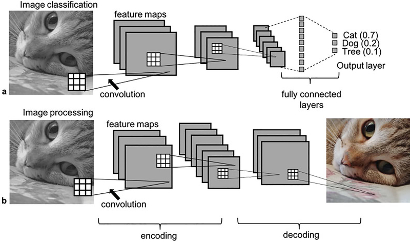
CNNs, ubiquitous in the field of computer vision, are a specific type of neural network in which the learned elements (weights) of the network form convolution kernels that extract features from the input image, illustrated in ►Fig. 1. The CNN learns to extract features that help it perform a task such as classifying an image. A CNN learns by comparing the output of the network with the target output; an error, or loss, is then calculated that measures the difference between the output and the target. The weights in the model are then updated to try to minimize this loss.

Fig. 1.

Illustration of example Convolutional Neural Network architectures. The network in a) takes the input image and performs classification based on image content. This decision is informed by learned features extracted from the image through the convolution operations. The square grids represent convolution kernels which are made up of trainable weights. Each voxel in a feature map is the result of a convolution operation applied to the previous layer (illustrated by the dotted lines). The network has 3 convolutional layers and 2 pooling layers; the choice of 3 or 6 channels in the convolution layers is an arbitrary choice in this didactic example. The network output is a vector of probabilities, where a probability is assigned to each class (ie. cat, dog, tree). The network in b) takes the input image and estimates the red green, blue components of the image, again based on learned features extracted from the image by the convolution kernels. An image processing CNN typically will have an encoder-decoder style architecture which contains pooling layers followed by upsampling layers. Both the networks in a) and b) are trained with many examples of input/output pairs; the weights in the network are continuously updated to minimize the difference between the output and target.

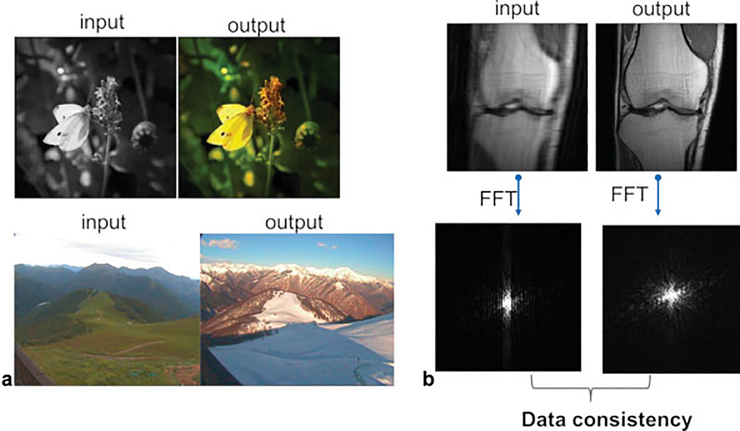
Although supervised deep learning with CNNs has been highly successful in medical imaging, leading to breakthroughs in the field of computer-aided diagnosis,^11,12 the potential for CNNs in computer vision and medical imaging goes beyond image classification. Outside the field of medical imaging, deep learning image enhancement has been used for many artistic applications such as those shown in ►Fig. 2a. In medical imaging, we can use deep learning to estimate a high-quality MR image from undersampled data. ►Fig. 2b shows an image reconstructed from undersampled data and the reference (fully sampled) output. Although the application of deep learning to diagnostic imaging is very different than these artistic applications, the tools used are similar. A key difference between generating an artifact-free MR image and the examples shown in ►Fig. 2a is the acquisition of the image in the Fourier domain (k-space). This provides a constraint on the generated image in that the sampled data in k-space should be the same for the input and output data. We can enforce this data consistency in our models, and several of the methods described in this article do make use of this.

Fig. 2.

Deep learning with convolutional neural networks (CNNs) has been used for artistic applications such as (a) colorizing a black-and-white image and predicting what a landscape will look like in the winter from an image of the same landscape in the summer. (b) Similar techniques can be used to predict a high-quality knee image from undersampled data. The main difference between the example in (b) and those in (a) is the acquisition of the image in k-space. The acquired k-space data of the input should match the corresponding data points in the k-space of the output, which can be enforced in deep learning reconstruction algorithms and is referred to as data consistency. FFT, fast Fourier transform.

Image-based Techniques for Reconstruction of Accelerated MR Images

One category of machine learning techniques that enables faster imaging operates in image space.^1,3,13 These methods are extensions of SENSE; they incorporate measured coil sensitivities in the reconstruction and were designed to generalize the concept of compressed sensing by learning the entire reconstruction procedure for MR data. Like traditional iterative reconstruction and compressed sensing, reconstruction methods based on deep learning make use of a regularization term that encompasses the prior information about the image content. However, deep learning allows us to learn this prior information from large amounts of data rather than defining it explicitly. Effectively, we learn prior information about the relationship between undersampled and fully sampled data, and prior information about the content and structure of fully sampled MR images.

A particularly successful image-based method for reconstructing accelerated image acquisitions is the variational network (VN) that was demonstrated for successful reconstruction of fourfold accelerated knee images.^3,14

Using the zero-filled reconstruction as the starting point, the VN solves the image reconstruction problem from the undersampled k-space by enforcing data consistency, application of the measured coil sensitivities, and using a CNN to learn the prior information and ultimately estimate the fully sampled image. It is essentially a deep learning extension of SENSE and compressed sensing. Example of VN reconstructions for fourfold accelerated images are shown in ►Fig. 3 along with the calculated structural similarity index measure (SSIM),¹⁵ an image similarity metric that quantifies the agreement with the ground truth. It is considered to be correlated with perceptual image quality. An SSIM value of 1 indicates perfect agreement. The VN reconstruction is also compared with a combined parallel imaging compressed sensing (PI-CS) reconstruction, the non–deep learning state of the art for reconstructing accelerated images.¹⁶

Fig. 3.

From left to right: A single slice of the reference, zero-filled, parallel imaging compressed sensing (PI-CS) and variational network (VN) reconstructions of a coronal proton-density-weighted knee image. The displayed structural similarity index measure values were calculated for the presented slice. The VN reconstruction has fewer residual artifacts than the PI-CS reconstruction.

The CNN portion of the VN in its original design is relatively shallow. A deeper CNN with more model capacity (more learnable parameters) may be able to learn more extensive prior information, potentially contributing to a more accurate reconstruction. Experiments were performed in which the CNN in the classic VN (approximately 131,000 learnable parameters) was replaced with a U-Net, a very popular network that has been successful in many medical imaging applications. The U-Net is a multilayer CNN with several encoding layers, followed by corresponding decoding layers. The U-Net-VN, with about 1.2 million learnable parameters, has a much larger model capacity compared with the classic VN. Sample reconstructions using the standard VN and a U-Net-VN, each trained with the same 30 image volumes (proton-density[PD]-weighted coronal knee images), are illustrated in ►Fig. 4. In a test set of 10 knee images, the average SSIM was 0.97 and 0.98 for the VN and U-Net-VN reconstructions, respectively. The U-Net reconstructions generally appear sharper and have fewer residual artifacts than the classic VN reconstructions.

Fig. 4.

From left to right: A single slice of the reference, zero-filled, parallel imaging compressed sensing (PI-CS), classic variational network (VN) and U-Net-VN reconstructions of a coronal proton-density-weighted knee image. The displayed structural similarity index measure values were calculated for the presented slice. Both the VN and U-Net-VN have improved image quality compared with the PI-CS reconstruction. The U-Net-VN outperforms the classic VN in that it is often sharper and has fewer residual artifacts.

PI-CS, and traditional iterative reconstruction methods in general, require a lengthy optimization step for the reconstruction of each individual image. In contrast, methods based on deep learning shift this optimization stage to an upfront training task, making the time-critical step of reconstructing a new clinical image very fast. Thus, in addition to offering improved reconstruction quality over PI-CS, deep learning–based reconstruction also has the benefit of very fast reconstruction times.

K-space–based Techniques for Reconstruction of Accelerated MR Images

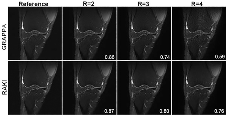
The previous section discussed deep learning methods that are applied in image space. It is also possible for deep learning techniques to be applied directly in k-space. Robust artificial-neural networks for k-space interpolation (RAKI) is a deep learning approach for improved k-space interpolation. Like GRAPPA, RAKI uses the fully sampled center of k-space, referred to as the autocalibration signal (ACS), and interpolation to estimate unsampled data points. However, RAKI uses CNNs, trained from ACS data, as the interpolation function. RAKI consistently outperforms traditional GRAPPA reconstructions. A sample result is shown in ►Fig. 5 where RAKI is compared with GRAPPA for twofold (R = 2), threefold (R = 3), and fourfold (R = 4) accelerations of a PD-weighted, fat-suppressed (FS) knee image. An advantage of RAKI over the methods discussed previously is that it is scan specific. The CNNs are trained from data of a single image and then used to reconstruct that image. This is advantageous because it does not require large training sets. A disadvantage of this method is the longer reconstruction times compared with methods in which the computationally intensive training is done upfront and the actual reconstruction of accelerated measurements can be computed very quickly.

Fig. 5.

The left column presents a single slice of the reference proton-density fat-suppressed (PD-FS) knee image. Columns 2, 3, and 4 show the undersampled reconstructions for acceleration factor (R) R = 2, R = 3, and R = 4. The top row shows the GRAPPA reconstructions, and the bottom row shows the RAKI reconstructions. The structural similarity index measure is higher for the RAKI reconstruction for all acceleration factors.

Adversarial Networks

A limitation with CNN reconstruction lies in the loss functions: minimizing pixel-wise loss metrics like mean squared error (MSE) or mean absolute error does not always result in natural-looking images; it is common for the generated images to appear oversmoothed.^17,18 The distinct difference in appearance can result in lower reader confidence. Generative adversarial networks (GANs) were developed to address this issue. They incorporate an adversarial loss, in addition to pixel-wise loss, that preserves the natural appearance of the images. This loss is learned via a second CNN, referred to as a discriminator, trained to distinguish between predicted images and fully sampled reference images. A GAN that enforces data consistency is described in Liu et al¹. Like all GANs, it consists of a CNN generator, simply a standard CNN with image input and image output, and a CNN discriminator. The discriminator is a classifier network, and in this specific GAN, the generator is the U-Net network previously discussed.

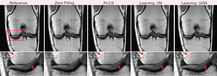
Unlike the other image-space methods that have a single pixel-wise loss function, the GAN has three loss terms. The first is the standard pixel-wise MSE loss between the generator output and the ground truth. The second is again a standard pixel-wise MSE loss, this time between the output and input k-space data. This loss term enforces consistency with the acquired data. The third loss term is the error in the discriminator (adversarial loss) that enforces the generation of images with a natural appearance. The generator and discriminator are trained simultaneously where the objective of the generator is to minimize the two pixel-wise loss terms and maximize the adversarial loss. The discriminator is trained to distinguish between the output and target images and minimize the adversarial loss. Examples of results from the data-consistent GAN described in Liu et al¹ are shown in ►Fig. 6. Although methods that incorporate adversarial loss may produce images with a more natural appearance, these networks are much more difficult to train and may increase the likelihood of hallucinating image features.¹⁹

Fig. 6.

Representative examples of knee images (coronal proton-density-weighted) obtained using the different reconstruction methods at acceleration rate R = 3. Compared with the traditional method with a combination of parallel imaging and compressed sensing (PI-CS) and the variational network (VN), the data-consistent generative adversarial network (GAN) provided better removal of aliasing artifacts in the bone and cartilage, and greater preservation of the sharp texture and tissue details, thus creating high-quality reconstructed images. The arrows indicate regions where tissue details are especially well preserved in the learned reconstructions.

Super-resolution

Image super-resolution refers to a class of techniques that enhance the resolution of images and videos. Deep learning–based image super-resolution is a promising approach for MRI where there is often a trade-off between resolution and scan time. Predicting high-resolution images from lower resolution images would be an effective way of accelerating MR acquisitions.

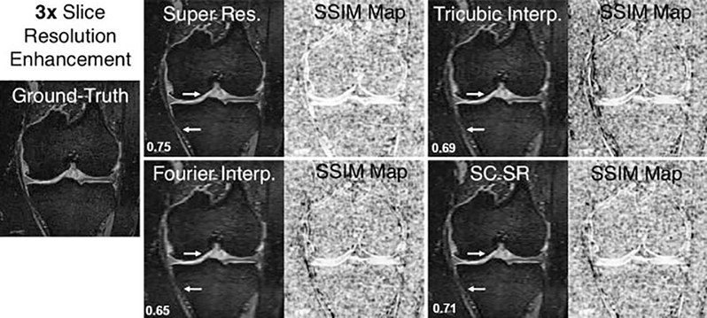
A three-dimensional (3D) CNN called DeepResolve⁴ learns transformations between high-resolution thin slice images and lower resolution thick slice images. DeepResolve was trained using 124 double-echo steady-state (DESS) knee data sets with 0.7-mm slice thickness. The high-resolution images (0.7 mm slice thickness) were the ground-truth reference images; the input images had between three- and eightfold larger slice thickness. The DeepResolve method of generating high-resolution thin slice images outperforms tricubic interpolation, Fourier interpolation, and sparse coding super-resolution,²⁰ a non–deep-learning super-resolution method, for all acceleration factors. An example of 3 times slice resolution enhancement is shown in ►Fig. 7.

Fig. 7.

Example of knee double-echo steady-state images showing 3× resolution enhancement in the slice direction (left to right) using the deep learning super-resolution method compared with conventional techniques such as Fourier interpolation, tricubic interpolation, and a state-of the-art non-deep learning technique of sparse coding super-resolution (SC SR). The accompanying structural similarity index measure (SSIM) maps demonstrate image quality differences compared with the ground-truth image (white = high similarity; black = low similarity). The arrows indicate regions of particular image quality enhancement around the articular cartilage and the medial collateral ligament. The calculated SSIM values are displayed in the bottom left corner.

Beyond Knee MRI

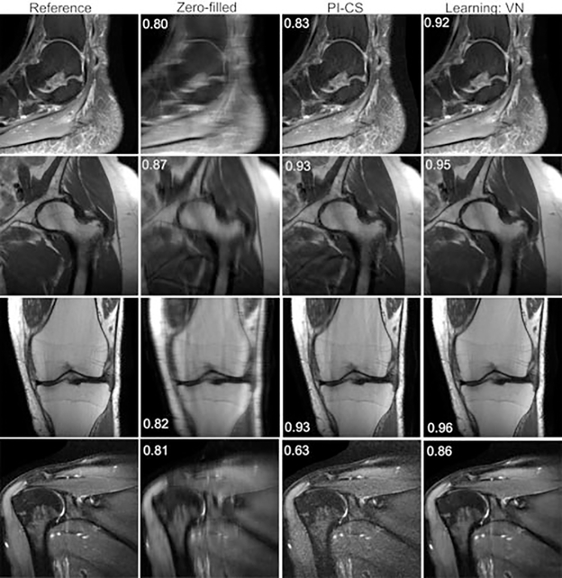
Knee imaging has been the main anatomical focus in the development and evaluation of deep learning–based reconstruction techniques for MSK MRI. It is important to assess the generalizability of deep learning reconstruction to other MSK applications. In this section we show the results of experiments evaluating the VN for reconstructions of fourfold accelerated shoulder, hip, knee, and ankle images. The VN was trained separately for each protocol with 30 training examples. Each trained network was tested on 10 retrospectively fourfold undersampled image volumes. All scans were performed on a clinical 3-T system (Siemens Magnetom Skyra), with different receive coils ranging from 12 to 26 elements. For all anatomical regions, the VN outperformed PI-CS. Samples of results are shown in ►Fig. 8.

Fig. 8.

Ankle (sagittal proton-density fat-suppressed [PD-FS]), hip (coronal PD), knee (coronal PD), and shoulder (T2-weighted FS) reconstructions with fourfold acceleration. The learned reconstructions appear sharper and have fewer residual artifacts than the parallel imaging compressed sensing (PI-CS) reconstructions. The displayed structural similarity index measure values were calculated for the presented slices.

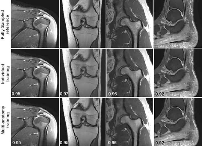
The results in ►Fig. 8 were obtained by training networks for a single anatomical region. It is currently an open question as to whether this specificity is necessary or if a single network can be trained for different types of images. The simplicity of a single network for a wide range of clinical applications would be a substantial benefit for clinical translation. Shown here are preliminary results for joint multi-anatomy training. A single VN was again trained with 30 images; however, this time the training set included six of each of five anatomical regions: ankle, knee, hip, shoulder, and brain. The network was then evaluated on each protocol and compared with the results of the individual networks. Generally, the multi-anatomy network approaches the performance of the anatomy-specific networks with only small differences in SSIM and perceived image quality. Example of results are shown in ►Fig. 9. An additional benefit of multi-anatomy training is the potential for much larger training sets.

Fig. 9.

Ankle (sagittal proton-density fat-suppressed [PD-FS]), hip (coronal PD), knee (coronal PD), and shoulder (T2-weighted FS) reconstructions with fourfold acceleration. The learned reconstructions appear sharper and have fewer residual artifacts than the parallel imaging compressed sensing (PI-CS) reconstructions. The displayed structural similarity index measure values were calculated for the presented slices.

Diagnostic Accuracy

The techniques presented in this article are all very promising for increasing the speed of MR examinations. They have been shown to produce high-quality images, assessed qualitatively, and with quantitative metrics such as SSIM. An important line of investigation is how the generated images compare with standard methods in terms of the reader’s diagnostic accuracy.

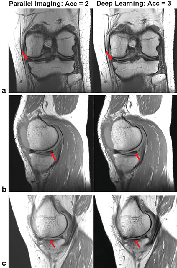
A clinical reader study by Knoll et al²¹ compared VN-reconstructed threefold accelerated knee images with the clinical standard, a twofold accelerated parallel imaging reconstruction, for the diagnosis of internal derangement of the knee. Ten MRIs were obtained for the training stage consisting of PD-weighted coronal and sagittal sequences. An additional 25 MRIs were acquired for testing. These examinations were ordered to evaluate for internal derangement. The 25 examinations were evaluated by three MSK radiologists and assessed for the presence of meniscal and ligament tears, articular cartilage defects, and signal abnormalities.

The results of the study show excellent concordance in the identification of internal derangement between parallel imaging and the VN-reconstructed images. Examples of images where pathology is clearly observed in both protocols are shown in ►Fig. 10.

Fig. 10.

A single slice of proton-density-weighted (a) coronal and (b, c) sagittal images from 3 different patients: TR/TE, 2,800/2, turbo factor (TF): 4, matrix size: 320 × 288 (coronal) and 384 × 307 (sagittal), on a 3-T system (Skyra, Siemens) using a 15-channel knee coil. (a) A tear in the medial meniscus, (b) a complex tear of the medial meniscus and cartilage thinning with subchondral marrow changes are visible in both the parallel imaging and the variational network deep learning reconstructions.

Benchmark Data Sets

Over the past 3 years, tremendous progress has been made in the development of deep learning approaches for accelerating MR imaging. Moving forward, it will be important to reproduce, validate, and compare these methods. To do this effectively, large public data sets and consistent evaluation metrics will be required. Research in computer vision applications, such as image classification, has greatly benefited from the availability of ImageNet. A similar benchmark MRI data set would be very valuable to the accelerated MRI research community.

The DeepResolve study discussed earlier used data from the Osteoarthritis Initiative, a longitudinal study for studying osteoarthritis progression.²² This public data set contains FS 3D DESS images. However, it does not include raw multichannel k-space data required for the development and evaluation of deep learning–based image reconstruction techniques.

The fastMRI data set²³ is a collection of raw multicoil k-space data; it contains coronal PD and PD-FS data sets from both 3-T and 1.5-T clinical scanners. The total number of MRI data sets in the fastMRI repository exceeds 1,500. Although the fastMRI data set is a valuable resource, it is still limited to only knee images. Additionally, the images were acquired at a single institution and on scanners from a single vendor.

Future Perspectives

The AI approaches presented in this article are all promising for improving the speed of MRI. These methods use two-dimensional (2D) CNNs to learn the relationship between undersampled and fully sampled MR data, or in the case of super-resolution, the relationship between low-resolution and high-resolution data. The CNN also learns prior information regarding the structure and content of MR images. Although these 2D methods show great promise, there is potential to leverage more prior information by extending these techniques to 3D. Adjacent slices share considerable information in terms of structure and contrast, and this mutual information could significantly improve the reconstruction. This concept is well known in compressed sensing, where greater acceleration factors can be achieved in 3D compared with 2D images.

Another way to leverage mutual information is with joint multi-contrast training. By jointly reconstructing data from multiple contrasts, we can again take advantage of the shared structural information. The CNN in the reconstruction networks may then be able to learn the relationship between images with different contrasts that will contribute to more prior information and could potentially improve the reconstruction.

A preliminary study by Knoll et al evaluated the diagnostic accuracy of a deep learning–based reconstruction approach by comparing reader agreement between the deep learning reconstructions and the standard reconstruction of clinical knee images. Their findings suggest that the protocols are essentially interchangeable for diagnostic purposes. Moving forward it will be important to assess all the deep learning reconstruction techniques for diagnostic accuracy. Specifically, it would be valuable to assess diagnostic accuracy by comparing reader diagnosis with a known ground truth obtained from arthroscopy.

The fastMRI data set is an open source repository of raw multichannel k-space data that could be more valuable if it was expanded to include data from other institutions, scanner vendors, and anatomical regions. A large heterogeneous benchmark data set for evaluating and comparing methods will almost certainly accelerate the development of accelerated MRI approaches.

Conclusion

Accelerating MRI acquisitions is an active area of research, motivated by the long acquisition times of current clinical protocols. AI based methods for accelerating MR acquisitions include under-sampled image reconstruction methods as well as super-resolution. Under-sampled image reconstruction methods can be applied in both image space and k-space and have shown promising results for MSK MRI applications. Promising directions for future development include, extending deep learning reconstruction models to use 3D CNNs and joint multi-contrast training, thoroughly evaluating the diagnostic accuracy of AI accelerated images to ensure that the clinical quality is not compromised, and expanding on available bench-mark datasets.

References

- 1.Liu F, Samsonov A, Chen L, Kijowski R, Feng L. SANTIS: Sampling-Augmented Neural neTwork with Incoherent Structure for MR image reconstruction. Magn Reson Med 2019;82(05):1890–1904 [DOI] [PMC free article] [PubMed] [Google Scholar]
- 2.Akçakaya M, Moeller S, Weingärtner S, Uğurbil K. Scan-specific robust artificial-neural-networks for k-space interpolation (RAKI) reconstruction: database-free deep learning for fast imaging. Magn Reson Med 2019;81(01):439–453 [DOI] [PMC free article] [PubMed] [Google Scholar]
- 3.Hammernik K, Klatzer T, Kobler E, et al. Learning a variational network for reconstruction of accelerated MRI data. Magn Reson Med 2018;79(06):3055–3071 [DOI] [PMC free article] [PubMed] [Google Scholar]
- 4.Chaudhari AS, Fang Z, Kogan F, et al. Super-resolution musculoskeletal MRI using deep learning. Magn Reson Med 2018;80(05): 2139–2154 [DOI] [PMC free article] [PubMed] [Google Scholar]
- 5.Griswold MA, Jakob PM, Heidemann RM, et al. Generalized autocalibrating partially parallel acquisitions (GRAPPA). Magn Reson Med 2002;47(06):1202–1210 [DOI] [PubMed] [Google Scholar]
- 6.Pruessmann KP, Weiger M, Scheidegger MB, Boesiger P. SENSE: sensitivity encoding for fast MRI. Magn Reson Med 1999;42(05): 952–962 [PubMed] [Google Scholar]
- 7.Sodickson DK, Manning WJ. Simultaneous acquisition of spatial harmonics (SMASH): fast imaging with radiofrequency coil arrays. Magn Reson Med 1997;38(04):591–603 [DOI] [PubMed] [Google Scholar]
- 8.Lustig M, Donoho D, Pauly JM. Sparse MRI: The application of compressed sensing for rapid MR imaging. Magn Reson Med 2007;58(06):1182–1195 [DOI] [PubMed] [Google Scholar]
- 9.Simonyan K, Zisserman A. Very deep convolutional networks for large-scale image recognition. 2014;1409:1556 [Google Scholar]
- 10.Szegedy C, Liu W, Jia Y, et al. Going deeper with convolutions. 2014. Available at: https://www.cs.unc.edu/~wliu/papers/GoogLeNet.pdf. Accessed October 7, 2019
- 11.Shin HC, Roth HR, Gao M, et al. Deep Convolutional Neural Networks for Computer-Aided Detection: CNN Architectures, Dataset Characteristics and Transfer Learning. IEEE Trans Med Imaging 2016;35(05):1285–1298 [DOI] [PMC free article] [PubMed] [Google Scholar]
- 12.Geras KJ, Wolfston S, Shen Y, et al. High-resolution breast cancer screening with multi-view deep convolutional neural networks. 2017. Available at: https://arxiv.org/pdf/1703.07047.pdf. Accessed October 7, 2019
- 13.Aggarwal HK, Mani MP, Jacob M. MoDL: Model-Based Deep Learning architecture for inverse problems. IEEE Trans Med Imaging 2019;38(02):394–405 [DOI] [PMC free article] [PubMed] [Google Scholar]
- 14.Knoll F, Hammernik K, Kobler E, Pock T, Recht MP, Sodickson DK. Assessment of the generalization of learned image reconstruction and the potential for transfer learning. Magn Reson Med 2019;81 (01):116–128 [DOI] [PMC free article] [PubMed] [Google Scholar]
- 15.Wang Z, Bovik AC, Sheikh HR, Simoncelli EP. Image quality assessment: from error visibility to structural similarity. IEEE Trans Image Process 2004;13(04):600–612 [DOI] [PubMed] [Google Scholar]
- 16.Knoll F, Bredies K, Pock T, Stollberger R. Second order total generalized variation (TGV) for MRI. Magn Reson Med 2011;65 (02):480–491 [DOI] [PMC free article] [PubMed] [Google Scholar]
- 17.Quan TM, Nguyen-Duc T, Jeong WK. Compressed sensing MRI reconstruction using a generative adversarial network with a cyclic loss. IEEE Trans Med Imaging 2018;37(06):1488–1497 [DOI] [PubMed] [Google Scholar]
- 18.Yang G, Yu S, Dong H, et al. DAGAN: Deep De-Aliasing Generative Adversarial Networks for fast compressed sensing MRI reconstruction. IEEE Trans Med Imaging 2018;37(06):1310–1321 [DOI] [PubMed] [Google Scholar]
- 19.Cohen JP, Luck M, Honari S. Distribution matching losses can hallucinate features in medical image translation. 2019. Available at: https://arxiv.org/pdf/1805.08841.pdf. Accessed October 7, 2019
- 20.Yang J, Wright J, Huang TS, Ma Y. Image super-resolution via sparse representation. IEEE Trans Image Process 2010;19(11): 2861–2873 [DOI] [PubMed] [Google Scholar]
- 21.Knoll F, Hammernik K, Garwood E, et al. Accelerated knee imaging using a deep learning reconstruction process. Paper presented at: Annual Meeting of the International Society of Magnetic Resonance in Medicine; April 22–27, 2017; Honolulu, Hawaii [Google Scholar]
- 22.Peterfy CG, Schneider E, Nevitt M. The osteoarthritis initiative: report on the design rationale for the magnetic resonance imaging protocol for the knee. Osteoarthritis Cartilage 2008;16(12): 1433–1441 [DOI] [PMC free article] [PubMed] [Google Scholar]
- 23.Zbontar J, Knoll F, Sriram A, et al. fastMRI: an open dataset and benchmarks for accelerated MRI. 2018. arXiv.1811:08839 [Google Scholar]