Scale Formation Under Blended Phosphate Treatment for a Utility With Lead Pipes

Abstract

US corrosion control practice often assumes that the orthophosphate component of blended phosphate corrosion inhibitors causes the formation of low-solubility lead–orthophosphate solids that control lead release into drinking water. This study identified the solids that formed on the interior surface of a lead service line and a galvanized steel pipe excavated from a system using a proprietary blended phosphate chemical. The scale was analyzed by X-ray diffraction, X-ray fluorescence, and scanning electron microscopy/energy dispersive spectroscopy. Instead of crystalline lead–orthophosphate solids, a porous amorphous layer rich in aluminum, calcium, phosphorus, and lead was observed at the lead pipe scale–water interface. Thus, the mechanism inhibiting lead release into the water was not a thermodynamically predictable passivating lead–orthophosphate scale, but rather an amorphous barrier deposit that was possibly vulnerable to disturbances. Galvanized pipe scales showed relatively crystalline iron and zinc compounds, with additional surface deposition of aluminum, phosphorus, calcium, and lead.

Utilities in the United States intending to control lead (Pb) release under the Lead and Copper Rule (LCR) often employ blended phosphates, which are proprietary mixtures of orthophosphate and polyphosphate. Yet little is known about the exact mechanism of protection by blended phosphates and no corrosion scale analyses for pipes in this type of system have been reported. This article describes findings from the analyses of a Pb and galvanized steel pipe scale that contradict theoretical expectations that blended phosphates primarily control Pb by forming simple crystalline Pb(II)–orthophosphate passivating films, and discusses the implications associated with using this chemical for corrosion control.

INTRODUCTION

Consumption of Pb-contaminated drinking water in the United States has been estimated to contribute from 20% to more than 85% of total Pb exposure from all Pb sources (Hanna-Attisha et al. 2016, Triantafyllidou & Edwards 2012). The greatest risk of Pb exposure is to infants, young children, and pregnant women (e-CFR 2017). Lead release from Pb-based plumbing materials into tap water has been linked to higher incidence of miscarriages and fetal death (Edwards 2014). Elevated blood lead (EBL) had been traditionally defined as blood lead greater than 10 μg/dL, but the Centers for Disease Control and Prevention reduced that threshold to a reference value of 5 μg/dL in 2012 (CDC 2012). Consumption of Pb-contaminated tap water can increase the percentage of young children with EBL (Hanna-Attisha et al. 2016, Triantafyllidou & Edwards 2012, Edwards et al. 2009) as well as simply increase the blood lead level itself (Ngueta et al. 2016, 2015, 2014; Levallois et al. 2014; Triantafyllidou & Edwards 2012). Even low Pb levels in blood may irreversibly affect neurological, endocrine, cardiovascular, and immunological systems (Levallois et al. 2014, Mandour et al. 2013, Bierkens et al. 2012, NTP 2012, Rhoads et al. 2012, Lanphear et al. 2005, Bryce-Smith et al. 1978).

Pb service lines.

Legacy Pb service lines are the largest source of Pb in tap water in the United States, in homes where they are present (Sandvig et al. 2008). Water utility surveys have attempted to estimate the number of Pb service lines that are in service (e.g., Cornwell et al. 2016, USEPA 1991). One of the higher estimates is that about 10 million Pb service lines were in use before the LCR (USEPA 1991), but this number may still be unrepresentatively low today. This is due to low response rates in the survey, variations in plumbing code requirements, poor utility databases/records, and poor documentation of the number of customer-side Pb service lines that have remained after decades of partial replacements.

Galvanized pipes.

Galvanized pipes have also been recognized as a source of sporadic Pb release into tap water. Lead may sorb onto corrosion products on galvanized pipe surfaces from upstream Pb service lines and solders (Pieper et al. 2017, McFadden et al. 2011, HDR Engineering 2009), and/or it may be present as a result of the remnant Pb content of the galvanized pipe coatings themselves (Clark et al. 2015, AWWRF & DVGW-TZW 1996, McFarren et al. 1977). The grade of zinc (Zn) historically used for galvanizing has been reported to contain 0.5–1.4% of Pb by weight (AWWRF & DVGW-TZW 1996). Lead measurements on the outside surface of uncorroded galvanized pipe were reported to be 1.6 ± 0.5% of Pb by weight (Pieper et al. 2017) and up to 1.8% of Pb by weight (Clark et al. 2015). The inside surface scale of galvanized pipes removed from a residence contained 0–0.8% of Pb by weight (Pieper et al. 2017).

LCR.

The 1991 LCR established a 90th percentile action level for Pb of 0.015 mg/L in 1 L first-draw tap samples after at least 6 h of stagnation (e-CFR 2017). The LCR was not designed to assess human exposure, but rather emphasizes corrosion control optimization to minimize Pb. Aside from meeting the Pb action level, water utilities under the LCR have to comply with state-approved optimal water quality parameter (OWQP) limits. Compliance status determines whether corrosion control treatment is properly operated and maintained for all large water systems, and for small and medium systems that exceed the action level. These water quality parameters include pH, alkalinity, calcium (Ca), and orthophosphate (when a corrosion inhibitor with an orthophosphate component is used).

Pb corrosion control with orthophosphate.

Utilities intending to control Pb release under the LCR may employ certain water treatment changes that induce the formation of less soluble compounds on the interior pipe wall. Aside from pH and/or alkalinity adjustment, among the most widely used approaches for corrosion control is orthophosphate addition, which has been shown to reduce Pb levels in comparison with systems without treatment (Cardew 2009, Hayes et al. 2008, Hozalski et al. 2005, Edwards & McNeill 2002).

The generally accepted theory for this mechanism of protection is the formation of low-solubility Pb(II)–orthophosphate solids, which bind the Pb to the scales on the pipe walls (Vesecky et al. 1997, AWWRF & DVGW-TZW 1996, Colling et al. 1992). Specifically, theoretical Pb solubility modeling in the presence of orthophosphate predicts formation of low-solubility Pb–orthophosphate solids such as chloropyromorphite (Pb₅(PO₄)₃Cl) and hydroxypyromorphite (Pb₅(PO₄)₃OH) (Figure 1), which have indeed been identified in corrosion scales of pipes from distribution systems using orthophosphate treatment (Schock et al. 2005, Davidson et al. 2004) and in corrosion scales of new Pb pipes used in experiments (Hopwood et al. 2002).

FIGURE 1.

Log activity-pH diagram for lead predicts formation of lead-orthophosphate solids

A 2001 survey of medium/large water utilities in the United States revealed that 56% used some form of phosphate corrosion inhibitors (McNeill & Edwards 2002). About 50% of those dosed with orthophosphate (as sodium or zinc orthophosphate), with the remaining 50% dosing pure polyphosphates alone or polyphosphates blended with orthophosphate.

Blends of orthophosphate with polyphosphate.

Pure polyphosphates, often a mixture of chain lengths and moieties (Boffardi & Sherbondy 1991, Holm & Schock 1991), have long been used as sequestering agents for iron (Fe) and manganese, but they have been reported to exacerbate corrosion of Pb plumbing materials (Edwards & McNeill 2002, Cantor et al. 2000, Holm & Schock 1991). Some reversion of polyphosphate to orthophosphate was shown to occur within distribution systems, though it was significant only in very hard water and long residence time (weeks) (Holm & Edwards 2003).

Blended phosphates are a mixture of orthophosphate and polyphosphate, with orthophosphate ranging widely in any given proprietary blend between 5 and 70% (USEPA 2016). Blended phosphates have been hypothesized to form passivating (i.e., protective) scales on the inner surface of Pb piping, with scale composition that is partially dependent on the water quality and with success that is dependent on scale thickness and stability (Friedman et al. 1994). The orthophosphate component of the blend is believed to be responsible for formation of the protective scales (Edwards & McNeill 2002, Lechner & Ziemba 1989).

However, other than some simple solubility modeling that roughly agreed with trends in metal release (Edwards & McNeill 2002), there is no direct confirmation of the mechanism by which blended phosphates act. In particular, there are no reported scale analyses for excavated Pb pipes in blended phosphate systems. In addition, theoretical Pb solubility modeling in the presence of the polyphosphate component is not possible, as it would be for pure orthophosphate (Schock 2004, 1985; Schock et al. 1996; AWWARF 1990). This is because solubility and formation constants of most polyphosphate species relevant to drinking water treatment are not available in the literature; the precise concentrations of these species are not known even by the manufacturer, and they may change with time as a result of reversion (Holm & Edwards 2003). Additionally, the polyphosphate species are not analytically determinable within the distribution system by standard water testing methods.

Study objective.

Characterization of the mineralogy and chemical composition of pipe scale deposits can show the relationship between scale formation and treatment history, and how this may influence Pb release into water over time (Sheiham & Jackson 1981). Scale analysis can also highlight the likelihood of the release of corrosion products resulting from physical disturbances (Del Toral et al. 2013). This study characterized the composition and morphology of scales formed on the interior surface of a Pb service line and a galvanized steel pipe from a Midwest surface water supply that has been employing blended phosphate corrosion control for over 20 years. This is the first examination of a Pb service line exposed to blended phosphate treatment. The main objective was to determine whether Pb(II)–orthophosphates were the dominant mineral phases formed on the Pb pipe scale, as theoretical solubility models would predict.

MATERIALS AND METHODS

Water quality.

Two treatment plants with similar finished water quality draw from one of the Great Lakes and serve approximately 5.4 million residents. Representative distribution system sampling in 2011 suggested that chlorinated hard water reached distribution system taps at a pH of 7.7–7.8, with a Ca content of up to 39 mg/L and an aluminum (Al) content of up to 0.11 mg/L (Table 1). Since 1993, blended phosphate has been added for corrosion control, with a 40%:60% ratio of orthophosphate:polyphosphate in the commercial proprietary blend. Total phosphate in tap water ranged between 0.84 and 1.2 mg/L as PO₄, with an average 90th percentile Pb level of 6 μg/L between 1999 and 2010 (Del Toral et al. 2013).

TABLE 1.

Main water quality parameters from sampling sites within the studied distribution system in 2011

Parametera	Range
Temperature—°C	5–23
Turbidity—ntu	0.10–0.35
pH	7.7–7.8
Chlorine residual (as Cl2)	0.70–0.91
Total alkalinity (as CaCO3)	98–110
Chloride	17–20
Sulfate	29–30
Hardness (as CaCO3)	140–150
Calcium	34–39
Orthophosphate (as PO4)	0.48–0.55
Total phosphate (as PO4)	0.84–1.2
Aluminum	0.029–0.11
Iron	<0.005–0.034

Adapted from Del Toral et al. 2013

CaCO₃—calcium carbonate

^aUnits are milligrams per liter unless otherwise noted.

Pipe samples.

Lead pipes.

Two sections of an excavated Pb service line (referred as pipes Pb-A and Pb-B) were obtained from a residence, totaling 44 in. in length with a 1 in. inner diameter and of unknown age.

Galvanized pipe.

Five sections of a galvanized steel pipe (collectively referred as pipe G) from premise plumbing downstream of a Pb service line were also obtained from a separate residence, approximately 10 mi from the location of the excavated Pb service line analyzed in this research. The galvanized pipe sections totaled 18.5 ft in length with a ¾ in. inner diameter. The exact galvanized pipe age is unknown, although the age of the residence was 84 years.

Pipe sample initial processing.

Pipes were shipped with the ends capped with threaded plugs to retain moisture in transit. All pipes were moist upon receipt at the US Environmental Protection Agency’s (USEPA’s) Advanced Materials and Solids Analysis Resources Core (AMSARC) laboratory in Cincinnati, Ohio. As of this writing, researchers at the AMSARC laboratory have analyzed more than 340 Pb pipe samples, harvested from 58 drinking water distribution systems spanning 18 US states and four Canadian provinces, following a refined in-house protocol and using an array of analytical techniques.

Initial processing involved plugging both ends with rubber stoppers, then cleaning the exterior surfaces with a wire brush and rinsing with deionized water to remove any loose debris. The rubber stoppers were removed and the pipes were laid out to dry for several days. Using a band-saw equipped with a steel blade (blade width ¼ in., 14 teeth/in.), the pipes were cross-cut into sections approximately 12 in. long. These sections were cut in half longitudinally to expose the inner surface of the pipe. The blade was cleaned with wood between each pipe sample, and separate blades were used for the Pb and galvanized pipes, to reduce the chance of cross-contamination.

Some Pb particles from the cutting process were scattered throughout the corrosion scale. These were removed as best as possible by gently tipping the pipes on end. Any runoff material was collected in plastic containers and later sieved to remove the metal particles. Recovered scale material was included in the total sample volume for the topmost layer of scale. Before harvesting the pipes, excess metal accumulated from the pipe-cutting process was gently removed with a small, stainless steel scalpel to further prevent contamination of scale materials. Any remaining metal shavings were removed during scale harvesting using fine-tipped forceps. Inevitably, some scale material was dislodged during transit and cutting. However, the amount was relatively small, and loose material was recovered when necessary.

Representative pipe sections (Figure 2) were selected and photographed using a digital camera to visually document the appearance of the corrosion scales. Reference pipe sections were then archived, while the remaining pipe sections were processed to be analyzed by a variety of analytical techniques (Figure 3). For “in situ” analysis, pipe cross sections were cut and the corrosion scale was otherwise left intact (Figure 3, left). For harvested corrosion scale analysis (scale no longer intact), pipe scales were examined under a stereo microscope to determine layer delineation, and the scale was carefully collected in layers (Figure 3, right).

FIGURE 2.

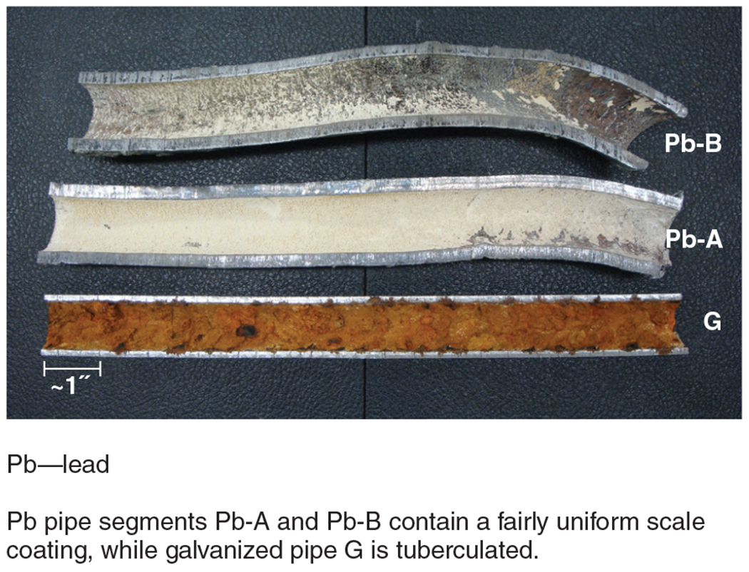
Internal corrosion scales of pipe samples that have been cut in half lengthwise

FIGURE 3.

Pipe sample processing and corrosion scale analyses at the US Environmental Protection Agency’s AMSARC laboratory

Pipe sample processing and analyses.

Scale layers were defined and sampled on the basis of differences in color and texture (Figure 3). The importance of harvesting and analyzing discrete scale layers instead of a single scraped bulk phase is explained in Schock et al. (2014). By convention, layer one (L1) denoted the outermost layer at the corrosion scale–water interface, which represents the most dynamic interactions with flowing water constituents. The underlying layers were numbered sequentially (i.e., L2, L3, L4), moving downward through the scale toward the pipe wall, and represent parts of the scale that are more isolated from direct water contact. Scale layers were harvested using brushes and fine-tipped, stainless steel tools. Care was taken to avoid mixing of sample layers while sampling. However, practical limitations precluded exact separation, and some cross-contamination between layers was inevitable during sample harvesting.

Material from each layer was ground by hand with an agate mortar and pestle to pass through a 200-mesh (75 μm) stainless steel sieve. Any layers with visible Pb or Fe pipe shavings from cutting were first passed through a 60-mesh (250 μm) sieve to remove metal particles. Powder sample materials for each layer were stored in glass vials. Aliquots of the powders were analyzed with a variety of techniques to characterize scale layers, while pipe cross sections of the intact corrosion scale were also analyzed (Figure 3).

Powder X-ray diffraction (XRD).

Mineral phases for each layer were determined via powder XRD (Figure 3, right). Sample material was evenly distributed on a quartz (SiO₂) or silicon zero-background sample holder. The diffractometer¹ used copper Kα radiation and had tube operating conditions of 45 kV and 40 mA. Samples were scanned from 10 to 90° 2θ with a 0.02° step size, and 60 s count time. XRD patterns were analyzed using appropriate software,² and diffraction data were compared against a reference database.³

X-ray fluorescence (XRF).

Pressed pellets were prepared to determine the bulk chemical composition of each layer (Figure 3, right). About 0.5–0.9 g of powder material for each layer was individually weighed on an analytical balance. Binder⁴ was added at nearly 10% by weight to permit cohesiveness of the material. All sample and binder weights were recorded and taken into consideration when processing analytical results. To ensure homogeneity, the powder/binder blend was mixed⁵ in a plastic container. Contents of the material were carefully poured into a detergent-cleaned and deionized water–rinsed stainless steel, 13 mm die set. An automated hydraulic die press⁶ was used for pressing the pellets, at operating conditions of 10 tons of pressure, 7.0 min hold time, and 2.0 min release time. After pressing, the pellet was inspected and handled with stainless steel forceps to determine the most homogeneous and smooth surface to be analyzed by XRF. Samples were analyzed by an XRF spectrometer,⁷ and the semi-standardless software routine was augmented by 20 certified standards incorporated into the calibration curves to better match the matrix of likely unknowns.

Total carbon and total sulfer.

Total carbon and total sulfur analysis was completed using a combustion furnace.⁸ Since binder was added to make pellets for XRF, this independent analytical determination of carbon (C) composition was inserted into the XRF calculation for C. The sulfur values were compared with those obtained using XRF to confirm that the concentrations were similar. This allowed for a comprehensive, unbiased elemental analysis.

Scanning electron microscopy/energy dispersive spectrometry (SEM/EDS).

Representative pieces of reference pipe were selected from each of the three samples for in situ analysis via SEM and EDS (Figure 3, left). SEM imaging allowed for observation of the surface morphology, while EDS enabled micro-elemental analysis of in situ layers. Additionally, EDS analyses on the cross sections were representative of undisturbed scale layers that are comparable to those collected for XRD and XRF analysis.

A section approximately 1 cm in length was cut and mounted in epoxy resin⁹ under −25 in. Hg vacuum, then cured at 50°C. Each epoxy mount was trimmed with a diamond saw.¹⁰ Separate blades were used for the Pb and galvanized pipe samples to avoid cross-contamination. The trimmed cross-sectional piece was then polished with 6 μm and 1 μm silicon carbide abrasive paper using a grinder/polisher.¹¹ The pieces were further polished using a cross-section polisher¹² with argon gas at 5.5 kV for 8 h.

Cross-sectioned regions were then examined using an SEM.¹³ An accelerating voltage of 10 kV was applied to obtain backscatter electron imaging, showing the distribution of different chemical phases in the sample.

Micro-elemental analysis using EDS was performed using an analytical drift detector.¹⁴ Using X-ray imaging, elemental line scans were performed vertically on an area of the cross section to show the elemental distribution across the scale layers. All elements were characterized with no normalization. Data were processed using appropriate software.¹⁵

Additionally, each cross section was used to obtain micro-scale images and determine the layer thickness using a digital microscope.¹⁶

RESULTS

Visual determination of corrosion scale layers.

Lead pipes.

In the Pb pipe segments Pb-A and Pb-B four scale layers were distinguished (Figure 4, parts A and B). L1 was white in color and up to 300 μm thick (Table 2). It was a loose, powdery surficial deposit that was mostly uniform. L1 was not well adhered to the underlying layer and could be easily removed with a small brush. L2 was slightly darker white in color and more compact than L1, with a thickness up to 40 μm. L2 was a fine-grained, nonuniform coating. L3 was up to 110 μm thick and dark brown in color, with patches of red, tan, and black. It consisted of a compact, coarser texture than L2. In areas where L2 was not present, L3 tended to flake off with L1. Additionally, L3 was absent in some areas. The layer closest to the pipe wall, L4, was glassy red to bright orange in color. It was a hard, uniform layer up to 200 μm thick and was strongly adhered to the pipe wall.

FIGURE 4.

Cross-sectional and macro-scale photographs of Pb-B pipe scale (A, B) and G pipe scale (C, D)

TABLE 2.

Color identification and approximate layer thickness for each layer of the pipe samples

Sample ID	Layer	Munsell Colora	Thickness μm
Pb-A	L1	10YR 8/1 white	35b
	L2	10YR 7/2 light gray
	L3	10YR 4/3 brown	30
	L4	10YR 6/4 light yellowish brown	200
Pb-B	L1	10YR 8/1 white	275–300
	L2	10YR 6/2 light brownish gray; 10YR 6/3 pale brown	40
	L3	10YR 2/2 very dark brown	110
	L4	10YR 6/4 light yellowish brown; 10YR 5/4 yellowish brown	150
G	L1	7.5YR 5/6 strong brown	35–80
	L2	10YR 4/2 dark grayish brown	700–1,800
	L3	7.5YR 3/2 dark brown	1,100–2,300

G—galvanized, ID—identification, L—layer, Pb—lead

^aDetermined under ambient laboratory lighting using the Munsell Soil Color Charts (2000) after scale was harvested

^bCombined thickness for L1 and L2

Galvanized pipe.

In the galvanized pipe G, three scale layers were distinguished (Figure 4, parts C and D). Given that the surface was heavily tuberculated, scale layers were not as discretely defined as in the Pb pipe segments. Additionally, the galvanized pipe scale was vastly thicker than that of the Pb scales (Table 2). The uppermost layer, L1, was red in color and up to 80 μm thick. L1 was a powdery layer that was easily removed with a brush. The middle layer, L2, was a dark blackish-brown to orange in color and up to 1.8 mm thick. L2 was compact and well adhered to the pipe wall. L3 was black or orange in color and up to 2.3 mm thick. It was the inner portion of the tubercles, which was a loosely adhered, coarse-grained material that sometimes exhibited magnetic properties.

Mineralogical characterization of corrosion scale layers.

Pb pipes.

XRD results for both Pb pipe segments were similar for all four layers (only L1 results are depicted here). Contrary to expectations, no crystalline Pb(II)–orthophosphates were detected in either Pb pipe segment. Instead, L1 was predominantly made up of a poorly crystalline or X-ray amorphous calcium aluminum phosphate CaAl₃(PO₄)(PO₃OH)(OH)₆ (crandallite H) (Figure 5), indicating that phosphorus (P) was binding with Ca and Al instead of Pb. L1 was also composed of the Pb(II)–carbonates PbCO₃ (cerussite) and Pb₃(CO₃)₂(OH)₂ (hydrocerussite), as well as the Pb(II)–oxide PbO (litharge) (Figure 5). Minor amounts of quartz and calcite (CaCO₃) were also detected (Figure 5).

FIGURE 5.

X-ray diffraction patterns for corrosion scale layer L1 (at the scale-water interface) of lead pipes Pb-A and Pb-B

It was not possible to determine whether the outer barrier layer was composed of a single compound with multiple anionic and cationic components of uniform and defined stoichiometry, or if it was a mixture of multiple compounds. This prevalence of ill-defined surficial deposits on pipes and relative absence of thermodynamically stable discrete Pb(II)–orthophosphate minerals, either at the surface or at depth in the pipe scale, is shared with observations of scales from multiple other phosphate-treated water systems previously analyzed by this laboratory (DeSantis & Schock 2014, DeSantis et al. 2012).

L2 was predominantly composed of the Pb–carbonates cerussite and hydrocerussite, the Pb(IV)–oxide polymorphs PbO₂ (plattnerite) and α-PbO₂ (scrutinyite), with minor amounts of calcite and quartz. L3 was composed of plattnerite and scrutinyite, with potential traces of cerussite. There was also an unidentified Pb mineral phase (or phases) that was of the cubic crystal system on L3. No Pb(II) or Pb(IV) reference patterns in the database matched the unidentified L3 peaks. L4 was predominantly composed of litharge.

Galvanized pipe.

L1 of the galvanized scale (Figure 6) was predominantly composed of Zn minerals, including Zn₂Al(OH)₆(CO₃)_0.5·H₂O and ZnFe₂O₄ (franklinite), with minor amounts of ZnO (zincite). L2 was composed of the Fe compounds FeCO₃ (siderite), Fe₃O₄ (magnetite), and γ–FeO(OH) (lepidocrocite). The innermost layer (L3) was predominantly siderite and magnetite. Note that the iron mineralogy may be somewhat incorrect because of the known tendency for transformations resulting from drying and air exposure (Świetlik et al. 2012).

FIGURE 6.

X-ray diffraction patterns for corrosion scale layer L1 (at the scale-water interface) of the galvanized pipe G

Elemental characterization of corrosion scales.

XRF analyses revealed fairly similar scale chemistry among the two Pb pipe segments, and notable variations between the Pb and galvanized pipes (Table 3).

TABLE 3.

Dominant elements of interest (weight percent) making up the corrosion scale layers

Sample ID	Layer	Al	Ca	Ca	Cl	Fe	Na	P	Pb	Zn
Pb-A	L1	16.0	0.9	7.4	0.04	2.2	0.1	12.1	14.6	0.02
	L2	14.1	1.4	5.8	0.1	0.4	0.1	8.6	30.0	0.03
	L3	5.0	1.6	1.2	<RL	0.4	<RL	2.3	62.7	0.03
	L4	<RL	0.6	0.1	0.2	0.1	<RL	0.1	83.7	0.03
Pb-B	L1	16.2	1.1	7.0	0.1	1.6	0.1	10.7	13.3	0.03
	L2	9.0	1.9	1.9	0.1	0.5	0.1	3.3	46.9	0.02
	L3	4.6	1.1	0.7	0.1	0.4	0.2	1.8	61.7	0.02
	L4	0.8	0.3	0.1	0.1	0.03	0.1	0.2	76.2	0.02
G	L1	4.2	1.9	1.4	0.2	31.3	4.3	2.7	0.8	21.7
	L2	0.5	1.5	0.8	0.05	56.5	1.3	0.2	0.1	5.8
	L3	0.6	3.0	0.2	0.08	55.6	1.6	0.1	0.1	7.8

<RL—below reporting limit, Al—aluminumn, C—carbon, Ca—calcium, Cl—chloride, Fe—iron, G—galvanized, ID—identification, Na—sodium, P—phosphorus, Pb—lead, Zn—zinc

^aCombustion analysis for carbon, X-ray fluorescence analysis for all other elements

Lead pipes.

Both Pb-A and Pb-B had appreciable amounts (in weight percent) of Pb, Al, P, and Ca (Table 3). L1 in Pb-A and Pb-B had substantial accumulation of Al (16%), P (11–12%), and Ca (7%). These elements were most abundant in L1 and decreased in concentration moving toward the pipe wall (Al ≤ 0.8%, P ≤ 0.2%, Ca = 0.1% in L4). Pb was the most abundant element in every layer of Pb-A and Pb-B, except L1, and increased toward the pipe wall (from 13–15% in L1 to 76–84% in L4). L1, L2, and L3 also contained small amounts of Fe and C, with even smaller amounts of chlorine. L4 was predominantly composed of litharge, with less than 0.8% of any other element.

Galvanized pipe.

The galvanized steel pipe contained 31–57% of Fe and 8–22% of Zn in all three layers (Table 3). L1 showed noteworthy accumulation of Fe, Zn, Al, sodium (Na), Ca, and P. These elements, excluding Fe, decreased in concentration toward the pipe wall. Some Pb was also present throughout the scale, ranging from 0.8% in L1 to 0.1% in L3.

Micro-elemental characterization of corrosion scale layers.

Backscatter SEM micrographs (Figures 7 and 8) were overlaid with qualitative EDS elemental line scans across representative cross sections of in situ scale layers (Figures 9 and 10). Scale layers comparable to those collected for XRD and XRF analyses were clearly identifiable.

FIGURE 7.

Scanning electron micrographs in backscatter mode of a representative section of the Pb pipe scale

FIGURE 8.

Scanning electron micrographs in backscatter mode of a representative section of L2 on the galvanized pipe scale

FIGURE 9.

Elemental line scan for pipe Pb-A using SEM-EDS

FIGURE 10.

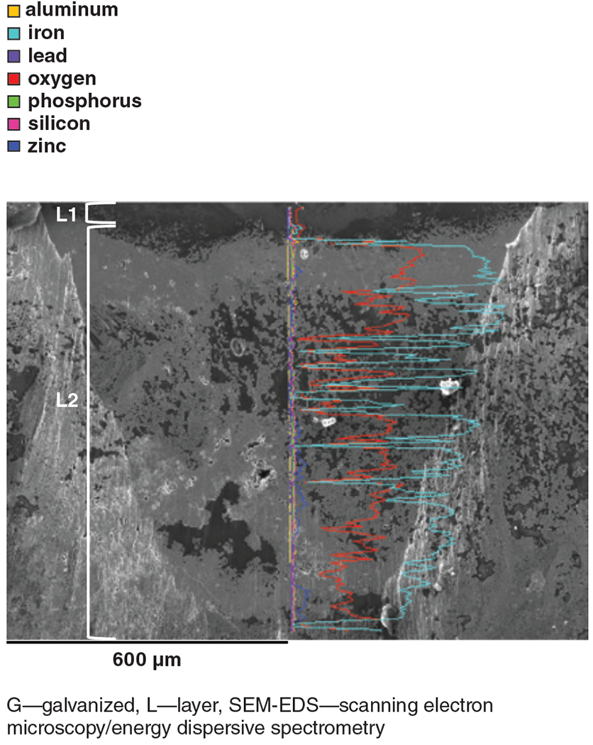
Elemental line scan for pipe G using SEM-EDS

Lead pipes.

For the two Pb pipe segments, backscatter SEM images revealed irregular patches of Pb-rich material near L1 (Figure 7). Additionally, L1 exhibited considerably more porosity than the underlying layers. SEM imaging of the cross sections also revealed intricate sublayering within L2 and L3, and poorly developed crystalline scales in all layers of both Pb segments.

Qualitative EDS elemental line scans across representative cross sections of in situ scale layers revealed Pb, P, Ca, Al, and oxygen (O). Pb intensities decreased upward through the scale, while Al, Ca, P, and O increased upward through the scale (Figure 9). Al, Ca, P, and O were found to penetrate through L3 (Figure 9). These results are in agreement with the XRF data.

Galvanized pipe.

SEM micrographs of pipe G revealed considerable porosity throughout all layers. L1 did not appear to be well crystalline. However, L2 and L3 contained well-defined crystal structures, with needle-like crystals in L2 (Figure 8) and plate-like crystals in L3. Complex sublayering was also observed throughout L2 and L3, which are not discretely divided layers. These observations of crystal habit could be an artifact of sample drying before analysis.

EDS data for pipe G (Figure 10) showed mostly Fe with peaks of P, Al, and silicon in the outermost layer. However, these elements were also detected within the lower layers, indicating water penetration beyond L1. Pb was also detected in all layers of the pipe G scales. C was detected in all line scans, but the data are not quantitatively reliable because of the carbon-based epoxy that was used for sample preparation. Overall, the qualitative elemental data from all EDS line scans are consistent with XRF data.

DISCUSSION

Deviation of Pb mineralogy from conventional theory.

The corrosion-scale mineralogy for Pb-A and Pb-B contradicts standard theoretical predictions based on thermodynamic equilibrium, which assume that the orthophosphate component in the water reacts with Pb from the pipe and scale to form simple low-solubility Pb(II)–orthophosphate solids (such as hydroxypyromorphite) that immobilize the Pb.

Notably, no crystalline hydroxypyromorphite or any other Pb(II)–orthophosphate compounds were detected in either Pb pipe segment. The innermost layers were composed of only Pb–carbonates and Pb-oxides. In this blended phosphate system, there may not be a sufficient ratio of orthophosphate to polyphosphate in the blend, or sufficient reversion of polyphosphate to orthophosphate in the distribution system, to induce the formation of Pb phosphate solids. Instead, an amorphous barrier containing Al, Ca, and P was the apparent mechanism of protection at the scale–water interface (i.e., in L1).

Potential impact of water treatment changes on Pb scale stability.

The co-occurrence of Al, Ca, and P on the outermost scale layer indicates that the phosphate available in the water reacts with Al and Ca (naturally present in the water; Table 1) before it can reach the pipe. This in turn raises the question of whether the amorphous barrier could destabilize if Al or Ca in the system are reduced as a result of treatment or other water quality changes, such as softening or switching to a non-Al coagulant. Pipes from Al-rich water supplies have been known to be latent reservoirs of heavy metals after treatment changes that reduce Al in the water (Snoeyink et al. 2003, Fuge et al. 1992). Additionally, sloughing off of the outermost layer would expose the inner Pb-rich corrosion layers and pipe wall.

Potential impact of physical disturbances on Pb release.

Physical evaluation of the scale composition of both the G and Pb pipes revealed porous, loosely adhered material at the scale–water interface that contained Pb. Del Toral et al. (2013) found that physical disturbances of Pb service lines in the same distribution system, including meter installation, leak repair, and road construction, were associated with elevated Pb levels at the tap. Figure 11 overlays tap water Pb profiles in undisturbed versus disturbed sampling sites from the Del Toral et al. (2013) study. Lead concentrations at several disturbed sites exceeded the LCR lead action level, while Pb concentrations at undisturbed sites fell mostly below the action level. Figure 11 also illustrates the broad range in lead concentrations found in the water in contact with the Pb service lines and other plumbing (as reflected by the different sequential water volumes sampled), for the same water treatment and water quality parameter conditions reflected in this study.

FIGURE 11.

Tap water lead profiles from the Del Toral et al. (2013) study, grouped in disturbed and undisturbed lead service line sites

If corrosion scales are not well adhered to the pipe wall, they are vulnerable to breaking away from the pipe from these kinds of disturbances, resulting in sporadic spikes in Pb levels at the tap that cannot be predicted and which may not be captured by the LCR sampling frequency (Del Toral et al. 2013), number of sampling sites/sampling protocol (Triantafyllidou & Edwards 2012), and water flow rate during sampling (Clark et al. 2014). Conceivably, physical disturbances or flow disruptions in galvanized premise plumbing could have a similar result, given that Pb was detected in these corrosion scales as well.

Comparison with prior studies of Pb coupon scale analysis.

Few compositional analyses have been performed on Pb corrosion products in water treated with blended phosphate. A group of researchers examined scale formation on Pb and copper coupons under blended phosphate treatment for different water quality conditions, though mineralogy was not examined directly (Vesecky et al. 1997; Friedman et al. 1995, 1994). Scale analysis was performed using X-ray photoelectron spectroscopy, infrared spectroscopy, and SEM.

Lead coupons exposed to blended phosphate in high-alkalinity (106–202 mg/L) and high-hardness (140–214 mg/L as CaCO₃) water contained Ca–phosphate solids, without Pb–carbonates or Pb–phosphates (Vesecky et al. 1997, Friedman et al. 1994). Coupons in low-alkalinity (10.2 mg/L) and low-hardness (11.6 mg/L) water contained large amounts of Fe, though the source was unknown (Friedman et al. 1995). The presence of P suggests the possibility of Fe orthophosphate in the scale. Masters and Edwards (2015) showed that particulate Fe deposition onto Pb pipes exacerbated lead release. Notably, coupons exposed to phosphoric acid (i.e., orthophosphate) treatment did not contain detectable amounts of Fe, but did have greater quantities of Pb and P.

These prior analyses agree with the results of this study in that the protective scale was an amorphous barrier composed of salts from other metals present in the water instead of being primarily composed of Pb phases. Scale formation did not align with theoretical predictions for orthophosphate, suggesting that the protection mechanism of blended phosphates is different from using orthophosphate alone.

Comparison with prior studies of galvanized pipe scale analysis.

The Zn and Fe minerals found in pipe G are in agreement with other examinations of galvanized pipes (Carbucicchio et al. 2008, Beccaria 1990, Myers 1973). The presence of Pb at the outermost layer of the corrosion scale may represent sorption from the upstream Pb service line or Pb from the galvanized pipe coating itself. Several studies have documented the sorption of inorganic contaminants on Fe corrosion scales (Pieper et al. 2017; McFadden et al. 2011, 2009; HDR Engineering 2009). The Pb content of the galvanized pipe scale examined in this study (0.1–0.8% Pb by weight depending on scale layer; Table 3) is in agreement with that reported by Pieper et al. (2017) for the interior pipe scale of an excavated galvanized service line.

Future treatment changes could result in destabilization of the existing corrosion scale, creating a latent source of Pb long after the primary source of Pb is removed. Particulate Pb could be released sporadically for years to come, and would be impossible to predict for any given tap water sample. Dissolved Pb could also be released as a result of desorption from the scale.

CONCLUSION

This work emphasizes the importance of pipe scale analyses in understanding corrosion control mechanisms. The morphology, mineralogy, and elemental composition of excavated pipe scales reflect water quality and treatment history and may even indicate vulnerability to Pb release from hydraulic, physical, and chemical changes or disturbances.

The mechanism inhibiting Pb release into the water with this blended phosphate treatment is not a single, discrete, passivating crystalline Pb(II)–orthophosphate phase. Rather, it appears to be a complex outer amorphous barrier deposit, originating by precipitation of components of the blended phosphate inhibitor with Al carry-over from coagulation and background water hardness and Fe content. This deposit contains Pb mixed with Al, Ca, P, Fe, and presumably light elements such as C, O, and hydrogen. This deposit may consist of one or more amorphous solid phases that probably also provide a barrier to Pb diffusion into the water from the underlying layers of more-crystalline Pb solids. The solids characterization methods available for this study were unable to distinguish whether there was a “pure” Pb(II)–phosphate phase disseminated within this complex amorphous deposit, which could affect Pb solubility and release.

Physically, this outer layer of the Pb pipes was porous and did not appear to be well adhered to the pipe wall. Scale could easily slough off with a small disturbance, sporadically releasing particulate Pb and exposing underlying layers high in Pb (similar to the situation illustrated in Figure 11) that would need considerable time to reestablish equilibrium with the flowing water.

The corrosion scale on pipe G contained relatively well-crystallized Fe and Zn compounds, with additional surface deposition of Al, P, and Ca, though not as much as on the Pb pipe segments. The G scale showed some Pb content, creating a potential reservoir of Pb release and extended time of Pb exposure, even if the upstream Pb pipe were to be removed from the distribution system.

Under the LCR (e-CFR 2017), compliance is determined by meeting state-designated OWQP limits. The stated purpose of the water quality parameters is that they will be “… those that the State determines reflect optimal corrosion control treatment for the system.” Further, “The State may designate values for additional water quality control parameters that the State determines to reflect optimal corrosion control for the system.”

This study found that the mechanism of Pb corrosion control by blended phosphate in this and potentially in other blended phosphate treated systems is not the formation of simple crystalline Pb(II)–orthophosphate minerals, predictable using only pH, alkalinity, and orthophosphate concentration. This suggests that water utilities need to conduct a demonstration study to determine the optimal chemical dosages and background water quality and treatment adjustments to minimize Pb release. There is no water chemistry basis to allow an a priori meaningful selection of all relevant water quality parameters in the first place, and the calculation or estimation of the impact on soluble or particulate Pb release of changes in OWQP concentrations in the bulk water. This and other studies (e.g., DeSantis & Schock 2014) showed that there are many background constituents in the water whose exact roles in influencing Pb release are unknown.

Because total Pb release in this and possibly other systems is not predictable from simple solubility equations, the effectiveness of corrosion control treatment can be evaluated only through a comprehensive tap water monitoring program that is designed to capture Pb release from the various leaded materials with which the water is in contact, and which customers would ingest.

Biography

Lauren W. Wasserstrom is an engineer at the American Water Works Association in Denver, Colo. She provides technical guidance and develops content on matters related to water quality and water research. At the time of this study, she was a graduate student researcher at the US Environmental Protection Agency (USEPA) in Cincinnati, Ohio, through a cooperative agreement with the University of Cincinnati. She conducted graduate research related to corrosion and metal accumulation in drinking water distribution systems. Wasserstrom earned her bachelor’s and master’s degrees in geology from the University of Cincinnati. Stephanie A. Miller is an environmental consultant at Trinity Consultants in Westerville, Ohio. Simoni Triantafyllidou is an environmental engineer at USEPA, Cincinnati, Ohio. Michael K. DeSantis is a post-doctoral Fellow at the Oakridge Institute for Science and Education, hosted at USEPA, Cincinnati. Michael R. Schock is a chemist at USEPA, 26 W. Martin Luther King Dr., Cincinnati, OH 45268 USA.

REFERENCES

- AWWARF (AWWA Research Foundation) & DVGW-TZW (Technologiezentrum Wasser), 1996. (2nd ed.). Internal Corrosion of Water Distribution Systems. AWWARF, Denver, & DVGW-TZW, Karlsruhe, Germany. [Google Scholar]
- AWWARF, 1990. Lead Control Strategies. AWWARF, Denver. [Google Scholar]
- Beccaria AM, 1990. Zinc Layer Characterization on Galvanized Steel by Chemical Methods. Corrosion, 46:11:906 10.5006/1.3580857. [DOI] [Google Scholar]
- Bierkens J; Buekers J; Van Holderbeke M; & Torfs R, 2012. Health Impact Assessment and Monetary Valuation of IQ Loss in Pre-School Children Due to Lead Exposure Through Locally Produced Food. Science of the Total Environment, 414:0:90 10.1016/j.scitotenv.2011.10.048. [DOI] [PubMed] [Google Scholar]
- Boffardi BP & Sherbondy AM, 1991. Control of Lead Corrosionby Chemical Treatment. Corrosion, 47:12:966 10.5006/1.3585211. [DOI] [Google Scholar]
- Bryce-Smith D; Mathews J; & Stephens R, 1978. Mental Health Effects of Lead on Children. Ambio, 7:5–6:192. [Google Scholar]
- Cantor AF; Denig-Chakroff D; Vela RR; Oleinik MG; & Lynch DL, 2000. Use of Polyphosphate in Corrosion Control. Journal AWWA, 92:2:95. [Google Scholar]
- Carbucicchio M; Ciprian R; Ospitali F; & Palombarini G, 2008. Morphology and Phase Composition of Corrosion Products Formed at the Zinc-Iron Interface of a Galvanized Steel. Corrosion Science, 50:9:2605 10.1016/j.corsci.2008.06.007. [DOI] [Google Scholar]
- Cardew PT, 2009. Measuring the Benefit of Orthophosphate Treatment on Lead in Drinking Water. Journal of Water and Health, 7:1:123 10.2166/wh.2009.015. [DOI] [PubMed] [Google Scholar]
- CDC (Centers for Disease Control and Prevention), 2012. What Do Parents Need to Know to Protect Their Children? www.cdc.gov/nceh/lead/acclpp/blood_lead_levels.htm (accessed February 2017).
- Clark BN; Masters SV; & Edwards MA, 2015. Lead Release to Drinking Water From Galvanized Steel Pipe Coatings. Environmental Engineering Science, 32:8:713 10.1089/ees.2015.0073. [DOI] [Google Scholar]
- Clark B; Masters S; & Edwards M, 2014. Profile Sampling to Characterize Particulate Lead Risks in Potable Water. Environmental Science & Technology, 48:12:6836 10.1021/es501342j. [DOI] [PubMed] [Google Scholar]
- Colling JH; Croll BT; Whincup PAE; & Harward C, 1992. Plumbosolvency Effects and Control in Hard Waters. Journal of the Institute of Water and Environment Management, 6:6:259 10.1111/j.1747-6593.1992.tb00750.x. [DOI] [Google Scholar]
- Cornwell DA; Brown RA; & Via S, 2016. National Survey of Lead Service Line Occurrence. Journal AWWA, 108:4:E182 10.5942/jawwa.2016.108.0086. [DOI] [Google Scholar]
- Davidson CM; Peters NJ; Britton A; Brady L; Gardiner PHE; & Lewis BD, 2004. Surface Analysis and Depth Profiling of Corrosion Products Formed in Lead Pipes Used to Supply Low Alkalintiy Drinking Water. Water Science and Technology, 49:2:49. [PubMed] [Google Scholar]
- Del Toral MA; Porter A; & Schock MR, 2013. Detection and Evaluation of Elevated Lead Release From Service Lines: A Field Study. Environmental Science & Technology, 47:16:9300 10.1021/es4003636. [DOI] [PubMed] [Google Scholar]
- DeSantis MK & Schock MR, 2014. Ground Truthing the ‘Conventional Wisdom’ of Lead Corrosion Control Using Mineralogical Analysis. Proc. AWWA 2014 Water Quality Technology Conference, New Orleans. [Google Scholar]
- DeSantis MK; Schock MR; & Bennett-Stamper C, 2012. Incorporation of Phosphate in Destabilized PbO2 Scales, Proc. AWWA 2012 Water Quality Technology Conference, Toronto. [Google Scholar]
- e-CFR (Electronic Code of Federal Regulations), 2017. National Primary Drinking Water Regulations. Title 40, Part 141, Subpart I, Control of Lead and Copper. www.ecfr.gov/cgi-bin/text-idx?tpl=/ecfrbrowse/Title40/40cfr141_main_02.tpl (accessed March 2017).
- Edwards M, 2014. Fetal Death and Reduced Birth Rates Associated With Exposure to Lead-Contaminated Drinking Water. Environmental Science & Technology, 48:1:739 10.1021/es4034952. [DOI] [PubMed] [Google Scholar]
- Edwards M; Triantafyllidou S; & Best D, 2009. Elevated Blood Lead in Young Children Due to Lead-Contaminated Drinking Water: Washington, DC, 2001–2004. Environmental Science & Technology, 43:1618 10.1021/es802789w. [DOI] [PubMed] [Google Scholar]
- Edwards M & McNeill LS, 2002. Effect of Phosphate Inhibitors on Lead Release. Journal AWWA, 94:1:79. [Google Scholar]
- Friedman RM; Cortez E; Liu J; Pacholec F; Lechner JB; & Dwyer JJ, 1995. Analysis of Film Formation Using Phosphate Inhibitors in Systems With Various Water Qualities. Proc. AWWA 1995 Water Quality Technology Conference, New Orleans. [Google Scholar]
- Friedman RM; Pacholec F; Powell RM; & Lechner JB, 1994. Blended Poly/orthophosphate Inhibition of Heavy Metal Corrosion in Potable Water Delivery Systems, Proc. AWWA 1994 Water Quality Technology Conference, San Francisco. [Google Scholar]
- Fuge R; Pearce NJG; & Perkins WT, 1992. Unusual Sources of Aluminum and Heavy Metals in Potable Waters. Environmental Geochemistry and Health, 14:1:15 10.1007/BF01783621. [DOI] [PubMed] [Google Scholar]
- Hanna-Attisha M; LaChance J; Sadler RC; & Champney Schnepp A, 2016. Elevated Blood Lead Levels in Children Associated With the Flint Drinking Water Crisis: A Spatial Analysis of Risk and Public Health Response. American Journal of Public Health, 106:2:283 10.2105/AJPH.2015.303003. [DOI] [PMC free article] [PubMed] [Google Scholar]
- HDR Engineering, 2009. An Analysis of the Correlation Between Lead Released From Galvanized Iron Piping and the Contents of Lead in Drinking Water Summary report, Bellevue, Wash. [Google Scholar]
- Hayes CR; Incledion S; & Balch M, 2008. Experience in Wales (UK) of the Optimisation of Orthophosphate Dosing for Controlling Lead in Drinking Water. Journal of Water and Health, 6:2:177 10.2166/wh.2008.044. [DOI] [PubMed] [Google Scholar]
- Holm TR & Edwards M, 2003. Metaphosphate Reversion in Laboratory and Pipe-Rig Experiments. Journal AWWA, 95:4:172. [Google Scholar]
- Holm TR & Schock MR, 1991. Potential Effects of Polyphosphate Products on Lead Solubility in Plumbing Systems. Journal AWWA, 83:7:74. [Google Scholar]
- Hopwood JD; Davey RJ; Jones MO; Pritchard RG; Cardew PT; & Booth A, 2002. Development of Chloropyromorphite Coatings for Lead Water Pipes. Journal of Materials Chemistry, 12:6:1717 10.1039/b111379h. [DOI] [Google Scholar]
- Hozalski RM; Esbri-Amador E; & Chen CF, 2005. Comparison of Stannous Chloride and Phosphate for Lead Corrosion Control. Journal AWWA, 97:3:89. [Google Scholar]
- Lanphear BP; Hornung R; Khoury J; Yolton K; Baghurst P; Bellinger DC; Canfield RL; et al. , 2005. Low-Level Environmental Lead Exposure and Children’s Intellectual Function: An International Pooled Analysis. Environmental Health Perspectives, 113:7:894 10.1289/ehp.7688. [DOI] [PMC free article] [PubMed] [Google Scholar]
- Lechner JB & Ziemba LM, 1989. Use of Blended Ortho/Poly Phosphate in Corrosion Control. Proc. AWWA 1989 Annual Conference and Exposition, Los Angeles. [Google Scholar]
- Levallois P; St-Laurent J; Gauvin D; Courteau M; Prevost M; Campagna C; Lemieux F; Nour S; D’Amour M; & Rasmussen PE, 2014. The Impact of Drinking Water, Indoor Dust and Paint on Blood Lead Levels of Children Aged 1-5 Years in Montreal (Quebec, Canada). Journal of Exposure Science and Environmental Epidemiology. 24:2:185 10.1038/jes.2012.129. [DOI] [PMC free article] [PubMed] [Google Scholar]
- Mandour RA; Ghanem AA; & El-Azab SM, 2013. Correlation Between Lead Levels in Drinking Water and Mothers’ Breast Milk: Dakahlia, Egypt. Environmental Geochemistry and Health, 35:2:251 10.1007/s10653-012-9480-0. [DOI] [PubMed] [Google Scholar]
- Masters S & Edwards M, 2015. Increased Lead in Water Associated With Iron Corrosion. Environmental Engineering Science, 32:5:361 10.1089/ees.2014.0400. [DOI] [Google Scholar]
- McFadden M; Giani R; Kwan P; & Reiber SH, 2011. Contributions to Drinking Water Lead From Galvanized Iron Corrosion Scales. Journal AWWA, 103:4:76. [Google Scholar]
- McFadden M; Reiber S; Kwan P; & Giani R, 2009. Investigation of Sorptive and Desorptive Processes Between Lead and Iron Corrosion Scales in Plumbing Materials. Proc. AWWA 2009 Water Quality Technology Conference, Seattle. [Google Scholar]
- McFarren EF; Buelow RW; Thurnau RC; Gardels M; Sorrell RK; Snyder P; & Dressman RC, 1977. Water Quality Deterioration in the Distribution System. AWWA 1997 Water Quality Technology Conference, Kansas City, Mo. [Google Scholar]
- McNeill LS & Edwards M, 2002. Phosphate Inhibitor Use at US Utilities. Journal AWWA, 94:7:57. [Google Scholar]
- Munsell Soil Color Charts, 2000. GretagMacbeth, New Windsor, N.Y. [Google Scholar]
- Myers JR, 1973. Corrosion of Galvanized Steel, Potable-Hot-Water Pipes, Hickam Air Force Base, Hawaii. Australasian Corrosion Engineering, May:29. [Google Scholar]
- Ngueta G; Abdous B; Tardif R; St-Laurent J; & Levallois P; 2016. Use of a Cumulative Exposure Index to Estimate the Impact of Tap-Water Lead Concentration on Blood Lead Levels in 1- to 5-Year-Old Children (Montreal, Canada). Environmental Health Perspectives, 124:3:388. [DOI] [PMC free article] [PubMed] [Google Scholar]
- Ngueta G; Gonthier C; & Levallois P, 2015. Colder-to-Warmer Changes in Children’s Blood Lead Concentrations Are Related to Previous Blood Lead Status: Results From a Systematic Review of Prospective Studies. Journal of Trace Elements in Medicine and Biology, 29:0:39 10.1016/j.jtemb.2014.07.004. [DOI] [PubMed] [Google Scholar]
- Ngueta G; Prévost M; Deshommes E; Abdous B; Gauvin D; & Levallois P, 2014. Exposure of Young Children to Household Water Lead in the Montreal Area (Canada): The Potential Influence of Winter-to-Summer Changes in Water Lead Levels on Children’s Blood Lead Concentration. Environment International, 73:57 10.1016/j.envint.2014.07.005. [DOI] [PubMed] [Google Scholar]
- NTP (National Toxicology Program), 2012. National Toxicology Program Monograph on Health Effects of Low-Level Lead. US Department of Health and Human Services, National Toxicology Program, Office of Health Assessment and Translation. [Google Scholar]
- Pieper K; Tang M; & Edwards M, 2017. Flint Water Crisis Caused by Interrupted Corrosion Control: Investigating “Ground Zero” Home. Environmental Science & Technology, 51:4:2007 10.1021/acs.est.6b04034. [DOI] [PubMed] [Google Scholar]
- Rhoads GC; Brown MJ; Cory-Slechta DA; Dietrich KN; Gardner SL; Gottesfeld P; Hansen K; Kosnett M; McCormick D; McKee-Huger E; Parsons P; Reyes B; Sandel M; & Williams D, 2012. Low Level Lead Exposure Harms Children: A Renewed Call for Primary Prevention, Centers for Disease Control and Prevention, www.cdc.gov/nceh/lead/acclpp/final_document_030712.pdf (accessed March 2017). [Google Scholar]
- Sandvig A; Kwan P; Kirmeyer G; Maynard B; Mast D; Trussell RR; Trussell S; Cantor AF; & Prescott A, 2008. Contribution of Service Line and Plumbing Fixtures to Lead and Copper Rule Compliance Issues. Research Report 91229. AWWA Research Foundation, Denver. [Google Scholar]
- Schock MR, 2004. Solubility Models and Their Limitations. AWWA 2004 Annual Conference and Exposition, Orlando, Fla. [Google Scholar]
- Schock MR, 1985. Treatment or Water Quality Adjustment to Attain MCLs in Metallic Potable Water Plumbing Systems EPA/600/9-85/007, US Environmental Protection Agency, Office of Drinking Water and Office of Research and Development, Cincinnati. [Google Scholar]
- Schock MR; Cantor A; Triantafyllidou S; Desantis MK; & Scheckel KG, 2014. Importance of Pipe Deposits to Lead and Copper Rule Compliance. JournalAWWA, 106:7:E336 10.5942/jawwa.2014.106.0064. [DOI] [Google Scholar]
- Schock MR; Lytle DA; Sandvig AM; Clement JA; & Harmon SM, 2005. Replacing Polyphosphate With Silicate to Solve Problems With Lead, Copper and Source Water Iron. Journal AWWA, 97:11:84. [Google Scholar]
- Schock MR; Wagner I; & Oliphant R, 1996. (2nd ed.). The Corrosion and Solubility of Lead in Drinking Water In Internal Corrosion of Water Distribution Systems. AWWA Research Foundation, Denver, & DVGW Forschungsstelle, Karlsruhe, Germany, 131–230. [Google Scholar]
- Sheiham I & Jackson PJ, 1981. Scientific Basis for Control of Lead in Drinking Water by Water Treatment. Journal of the Institute of Water Engineers and Scientists, 35:6:491. [Google Scholar]
- Snoeyink VL; Schock MR; Sarin P; Wang L; Chen AS-C; & Harmon SM, 2003. Aluminum-Containing Scales in Water Distribution Systems: Prevalence And Composition. Journal of Water Supply: Research and Technology—Aqua, 52:7:455. [Google Scholar]
- Świetlik J; Raczyk-Stanisławiak U; Piszora P; & Nawrocki J, 2012. Corrosion in Drinking Water Pipes: The Importance of Green Rusts. Water Research, 46:1:1 10.1016/j.watres.2011.10.006. [DOI] [PubMed] [Google Scholar]
- Triantafyllidou S & Edwards M, 2012. Lead (Pb) in Tap Water and in Blood: Implications for Lead Exposure in the United States. Critical Reviews in Environmental Science and Technology, 42:13:1297 10.1080/10643389.2011.556556. [DOI] [Google Scholar]
- USEPA (US Environmental Protection Agency), 2016. Optimal Corrosion Control Treatment Evaluation Technical Recommendations for Primacy Agencies and Public Water Systems. EPA 816-B-16–003. USEPA Office of Water (4606M), Cincinnati. [Google Scholar]
- USEPA, 1991. Final Regulatory Impact Analysis of National Primary Drinking Water Regulations for Lead and Copper Prepared by Wade Miller Associates Inc. & Abt Associates Inc. EPA Contract 68-C0-0069 Work Assignment No. 0-2. USEPA, Washington. [Google Scholar]
- Vesecky SM; Jingyue L; Friedman M; Pacholec F; & Lechner JB, 1997. Comparison of Film Formation Using Phosphate Inhibitors in Systems With Comparable Water Qualities. Journal of the New England Water Works Association, 111:3:258. [Google Scholar]