Life satisfaction, loneliness and togetherness, with an application to Covid-19 lock-downs

Abstract

Using the 2012–2013 American Time Use Survey, I show that both “who” people spend time with and “how” they spend it affect their life satisfaction, adjusted for numerous demographic and economic variables. Life satisfaction among married individuals increases most with additional time spent with one’s spouse. Among singles, satisfaction decreases most as more time is spent alone. Additional time spent sleeping or TV-watching reduces satisfaction, while longer usual workweeks and higher incomes increase it. Nearly identical results are shown using the 2014–2015 British Time Use Survey. The US estimates are used to simulate the impacts of Covid-19 lock-downs on life satisfaction.

Introduction

A substantial economics literature has arisen examining the determinants of human life satisfaction, arguably going back to Pollak (1976), with the early literature summarized by Easterlin (2001).1 Throughout this immense literature, however, very few studies have related satisfaction even to reports on work time in annual or monthly household surveys. The relationship between “how” one spends non-work time and happiness has also been studied (e.g., Kahneman et al. 2004). No study, however, has examined how the nature of a person’s interactions with others—“with whom” they spend their non-work time—relates to life satisfaction; and none has simultaneously examined how uses of time and with whom it is spent affect happiness or life satisfaction. I examine these relationships here, parsing out the determinants of satisfaction in two major population groups, married couples without young children, and singles.

Section II links the discussion to consumer theory. Section III describes the data and samples used to study how different relationships to the people with whom one spends time and how one uses it affect life satisfaction. Section IV presents sets of estimates based on these data, while Section V presents a confirmation using British time-use data. Since the widespread lock-downs associated with Covid-19 alter “with whom” one spends time, and probably also change “how” one spends it, Section VI reports the results of simulations of possible impacts of lock-downs on well-being using the American results.

A theoretical consideration

Neoclassical consumer theory has agents maximizing utility defined over goods/services. Becker’s (1965) generalization of the theory re-defined the maximand as being over “commodities”—home-produced combinations of purchased goods and the time inputs of household members. The theory is extremely powerful, as differences in the price of time across agents, proxied by their wage rates, have allowed predictions about behavior that can be linked to observables.

For many commodities one can also imagine that the consumer chooses with whom to produce and consume the commodity. For example, the leisure activity, attending a sporting event, could be produced alone, with one’s spouse/partner, with friend(s), or with a relative. Television-watching similarly offers the choice of “who with,” typically alone, with spouse/partner and/or other relatives (children). In the category of home production, laundry or house-cleaning are typically done alone or with one’s spouse/partner. Among other personal activities, although information on whom they are accomplished with is not included in the data sets used here, sexual activity might be undertaken alone, with spouse/partner or with a friend. In each case, with the same amount of goods and time devoted to the activity, the pleasure derived could vary depending upon who is present while the activity is undertaken.

These examples and myriad others suggest an expanded utility function:

$$U=U\left(Z_1\left(X_1,T_1,W_1\right),\dots ,Z_i\left(X_i,T_i,W_i\right),\dots ,Z_N\left(X_N,T_N,W_N\right)\right),$$

where Z_i is one of N commodities, X_i and T_i are the goods and time inputs into producing Z_i, and W_i is a vector of indicators of the identity(ies) of the individuals, if any, with whom Z_i is produced. I do not try to operationalize the theory here. One might, however, imagine the consumer choosing (or household members bargaining over) the combinations of goods to enjoy, time to allocate to each good and with whom to “produce” the Beckerian commodity. Just as the theory of household production is testable because of people’s different time prices, to make an expanded theory testable one would need to identify “prices” of the different choices of “who with” that vary across agents. Such “prices” might usefully be related to some proxies for the closeness or lack thereof of relationships with people with whom one might spend time. The only point here is that thinking about this extension is a reasonable rationalization for the empirical work. Like choices about spending time and purchasing goods and services, “who with” is an outcome of consumer choice.2

Data on “Who With” and life satisfaction

The basic data used in what follows come from the American Time Use Survey (ATUS) (produced by the US Bureau of Labor Statistics, discussed by Hofferth et al. 2018, with more detail presented by Hamermesh et al. 2005). Respondents are individuals who had recently (within 2–5 months, averaging 3 months) been included in the 8th wave of the monthly Current Population Survey. Only one adult per household is included (so that in married couples we only observe the husband or the wife, not both); and each respondent keeps a diary for only one day of the week (with 10% of diaries assigned for completion on each weekday, 25% on each weekend day).

In each year of its existence (beginning in 2003), in addition to tabulating the amount of time that respondents had spent during the previous day in a very detailed classification of activities (over 400), the ATUS asked people to record who they were with during many of the activities (sleep was excluded from the “who-with” list, as were other personal activities and some less frequent/lengthy activities). While the quantities of time spent in various activities in the ATUS have been analyzed many times (summarized in Hamermesh 2019), the “who with” information has received very little attention (with Flood and Genadek 2016, being a rare exception).

In 2012 and 2013 the ATUS fielded a Well-being Module, asking people questions about their feelings, including a question asking them to “think about your life in general” and rate their life satisfaction on a 10 (highest, “best possible life”) to 0 (lowest, “worst possible life”) scale—a Cantril “well-being ladder.”3 In the literature on life satisfaction various terms—life satisfaction, happiness and subjective well-being—appear to be used somewhat interchangeably. Since the available data refer specifically to life satisfaction, not happiness, I use the term “life satisfaction” and abbreviate it with the term “satisfaction.”

We know (Abraham et al. 2006) that respondents in the ATUS are not observationally different from all people asked to complete a diary. In the 2012 and 2013 rounds of the ATUS 23,657 people kept time diaries, of whom 21,589 completed the well-being ladder. There is no statistically significant difference between the demographic characteristics of the less than 10% of the samples used here who did not complete the well-being ladder and those of the large majority who did.4

I classify the usable observations by their marital status, distinguishing between those listing themselves as married with spouse present, and singles—those who list themselves as widow/ers, divorced or never married. Because “how” and “who with” differ if children are in the home, I create a sample of married individuals with no children under age 18. The second sample consists of single individuals with no children under 18 who are age 30 or over (to exclude many of those who may be living with roommates or cohabiting).5 With these restrictions the married—no children group contains 4710 respondents, and the singles group includes 6848 individuals. I thus study the behavior of slightly more than half the available ATUS sample and of the US adult population. The information on “who with” is collected in over 20 categories, ranging from spouse through more distant relatives, friends, different types of other people standing in various relationships to the respondent, and being alone. I aggregate this information into 5 categories: Alone; with friends; with other people; with other (non-spouse) relatives, or with spouse, with the last obviously not relevant in the sample of singles.

The distributions of “who with” in the samples are reported in the upper part of Table 1, for each sample and then for sub-samples distinguished by gender.6 For each category the table lists the minutes spent on a representative day and their standard deviation. Also included is the total amount of time per day for which “who with” is accounted and the age of respondents in each group. In both samples the average respondent is in his/her 50 s—among married respondents, because I exclude those with young children, and among singles because people under age 30 were excluded. Married individuals classify “who with” during about 51% of the day, about 1 h more than do singles. Women classify slightly less of their time as to whom they were with than men, a larger difference among singles than among married respondents.

Table 1.

Descriptive statistics, time spent alone and with others (minutes/day), and life satisfaction, ATUS 2012–2013^a

	Married, no children			Single ≥ 30, no children
“Who With”	All	Men	Women	All	Men	Women
Alone	275.9 (178.0)	281.5 (180.4)	270.3 (175.5)	371.8 (178.9)	367.6 (180.4)	375.1 (177.7)
With friends	27.7 (80.1)	28.4 (80.3)	27.0 (80.0)	62.6 (136.2)	73.1 (147.8)	54.3 (125.8)
With other people	135.2 (221.8)	143.2 (230.7)	127.2 (212.2)	154.6 (238.1)	174.9 (250.6)	138.6 (226.6)
With other relatives	33.0 (103.6)	25.1 (90.2)	40.9 (115.1)	85.0 (178.2)	73.9 (169.1)	93.7 (184.6)
With spouse	267.0 (238.0)	268.9 (242.0)	265.0 (233.9)	–	–	–
Total time with	738.8 (195.4)	747.0 (197.3)	730.4 (193.2)	673.9 (212.0)	689.5 (215.2)	661.7 (208.7)
Age	58.1 (13.7)	59.0 (13.9)	57.2 (13.4)	56.2 (15.4)	51.6 (14.5)	59.9 (15.0)
Life satisfaction (percent distributions)
10 (highest)	17.0	13.8	20.4	14.7	12.3	6.6
9	11.9	11.0	12.8	6.1	4.7	7.3
8	27.2	27.9	26.5	21.0	19.7	22.0
7	16.1	18.4	13.7	16.6	18.0	15.6
6	9.2	9.8	8.6	10.9	12.5	9.6
5	12.3	12.0	12.6	17.5	17.6	17.4
0–4 (lowest)	6.3	7.1	5.4	13.2	15.2	11.5
N =	4710	2332	2378	6848	2825	4023

^aStandard deviations in parentheses below means of “who with” and age

Married individuals report about 4–1/2 daily hours with a spouse (remembering that time sleeping is not included in these reports). That the married men and women are from separate couples creates a small, statistically insignificant gender difference in reported time with spouse. The other major category of “who with” is time alone, about 4–1/2 h per day, with men reporting significantly more (about 10 min/day) than women. The other categories account for much less time, about 1/2 h with friends (no gender difference), 2–1/4 h with other people (significantly more by men) and about 1/2 h with other relatives (significantly more by women). Among single individuals ages 30+ time spent alone accounts more than half of the over 11 daily hours for which respondents list “who with,” with men reporting slightly less time alone. About 2–1/2 h are spent with other people and 1 h with friends (more by men in both), and 1–1/2 h with other relatives (more by women). All these gender differences are statistically significant.

The bottom part of Table 1 displays the distributions of responses on the well-being ladder. As is standard in the literature, the majority of respondents say they are quite satisfied with their lives, with 33% (single men) being the largest fraction in any group reporting themselves in the bottom part of the ladder (life satisfaction below 6). Married individuals report greater well-being than singles, and within each sample women report greater well-being than men. Neither difference is standardized for other demographic characteristics, and there is at least some disagreement in the literature about the direction of any married-single difference in satisfaction (e.g., Knabe et al. 2010; Gimenez-Nadal and Molina 2015).

Impacts of “Who With” and “How” of time on life satisfaction

There are major demographic differences within each sample and sub-sample that are likely to relate to satisfaction and to how and with whom people spend time. We know that there is an inverse-U shaped relationship between age and time spent working for pay; gender and racial/ethnic differences in the allocation of time across activities; and differences by educational attainment, geography and day of the week and month of the year (Hamermesh 2019). I account for these differences by estimating for each sample linear regressions describing the 0–1 variable satisfied (score on the well-being ladder of 8 or above, accounting for 56% of the married sample, 42% of singles).

Main results

The initial least-squares estimates are in Columns (1) and (4) of Table 2.7 In each case the parameter estimates show the impact of an additional 100 min spent in the manner indicated. Each equation includes large numbers of covariates describing the respondent’s age, education, race/ethnicity, and location.8 Also included are household income and the individual’s usual weekly work hours (retrospectively reported), and a vector of measures of the allocation of time across activities (paid work, home production, sleep, other personal care and television-watching, with other leisure activities the excluded category). (The estimates of the impacts of the “who with” variables change little if this second group of covariates is excluded).

Table 2.

Estimates of the relation of with whom time is spent—alone and with others—to life satisfaction, ATUS 2012–2013^a

	Married, no children			Single ≥ 30, no children
	(1)	(2)	(3)	(4)	(5)	(6)
	All	Men	Women	All	Men	Women
Ind. Var. (in 100 min/day)
Alone	−0.0065 (0.0059)	−0.0094 (0.0086)	−0.0035 (0.0084)	−0.0121 (0.0044)	−0.0030 (0.0069)	−0.0199 (0.0058)
With friends	0.0140 (0.0095)	0.0054 (0.0139)	0.0170 (0.0136)	−0.0004 (0.0048)	−0.0026 (0.0070)	0.0023 (0.0068)
With other people	0.0021 (0.0059)	0.0053 (0.0081)	−0.0069 (0.0094)	−0.0039 (0.0041)	−0.0066 (0.0059)	−0.0021 (0.0059)
With other relatives	−0.0062 (0.0080)	−0.0049 (0.0129)	−0.0088 (0.0106)	0.0044 (0.0039)	0.0142 (0.0064)	0.0001 (0.0051)
With spouse	0.0144 (0.0046)	0.0153 (0.0066)	0.0164 (0.0068)	–	–	–
p on F-statistic of “who with” vector	<0.0001	0.002	0.004	0.004	0.044	0.002
Adj. R2	0.059	0.070	0.061	0.088	0.098	0.094
N=	4710	2332	2378	6848	2825	4023

^aStandard errors in parentheses. Additional covariates are: vectors of age indicators, years of educational attainment, racial/ethnic identity; measures of household income and the distribution of time spent on the diary day among work, home production, sleep, other personal care and TV-watching (with other leisure activities the excluded category); usual weekly hours of paid work, and vectors of indicators of class of worker, state of residence, day of week, month of year, year and immigrant status

In the married sample (Column (1)) time spent alone or with other relatives reduces satisfaction, while time spent with friends, other people or one’s spouse increases it. The positive effects of time with spouse are statistically significant; and the impact of time with friends approaches statistical significance.9 Overall, holding these demographic, geographic and temporal measures constant, people’s choices of “who with” are highly significantly related to their satisfaction. In the sample of singles (Column (4) of Table 2), more time alone has a highly significant negative impact on satisfaction. Additional time spent with other relatives has a positive effect on satisfaction, while additional time with friends or other people has negative effects, although none of these last three is statistically significant.10 Taken together, the indicators of “who with” also significantly affect the satisfaction of single individuals.

Switching 100 min (of a daily average of 276 min) from time alone to time with one’s spouse raises the probability that a married person is satisfied (well-being ladder at least 8) by 2.1 percentage points (on a mean of 56.1%), adjusting for all the demographic, time use and economic control variables. Among singles, switching 100 min of time spent with other people (on a mean of 155 min) to time spent alone reduces the probability that one is satisfied with life by 0.8 percentage points (on a mean of 41.8%). The impacts of who one spends time with on satisfaction are not only statistically significant, they are also not tiny.

The samples remain usably large if we disaggregate by gender. Estimates of the models shown in Columns (1) and (4) separately by gender are presented in Columns (2), (3), (5) and (6) of Table 2. Being alone bothers married men more than married women; being with friends raises married women’s life satisfaction more. Most important, the positive impacts of additional time with spouse are nearly identical between men and women; and there are no significant differences in the impacts of any of the other “who with” measures by gender. That is not true among singles: the negative impact of time spent alone shown in Column (4) of Table 2 results almost entirely from women being very much less satisfied with life as time spent alone increases. This negative effect is significantly different from the small negative effect among men. On the other hand, the small positive effect on life satisfaction among all singles of time spent with other relatives arises because men’s satisfaction increases significantly while women’s is unaffected.

One’s choices about “who with” depend in part upon “how” one spends time. For examples, with more time working for pay it is likely that one will spend less time with one’s spouse; with more time in home production one is less likely to spend time with friends. Given these relationships, however, even if choosing “how” precedes “who with,” the choices may still be somewhat independent, as the examples in Section II suggested. Since these effects are also of interest, Table 3 shows the means and standard deviations of these measures—income, weekly work time and the allocation of time on the diary day—and their estimated impacts on life satisfaction in the equations presented in Columns (1) and (4) of Table 2.

Table 3.

Descriptive statistics, and parameter estimates of the impacts of time spent in different activities, of usual hours and of family income on life satisfaction, ATUS 2012–2013^a

	Married, no children (N = 4710)		Single ≥ 30, no children (N = 6848)
	(1)	(2)	(3)	(4)
	Mean (s.d.)	a	Mean (s.d.)	b
Time-diary variables, in 100 min/day in Columns (2) and (4)
Home production	190.1 (172.5)	0.0046 (0.0054)	167.0 (165.4)	0.0029 (0.0044)
Sleep	512.9 (117.1)	−0.0167 (0.0072)	525.1 (139.4)	−0.0140 (0.0051)
Other personal care	129.6 (84.4)	−0.0002 (0.0093)	120.2 (90.6)	−0.0014 (0.0070)
TV-watching	187.2 (175.5)	−0.0154 (0.0054)	217.2 (224.1)	−0.0070 (0.0038)
Other leisure	216.4 (197.8)	–	224.1 (207.63)	–
Paid work	203.3 (274.3)	−0.0001 (0.0057)	186.4 (269.6)	−0.0073 (0.0045)
Other variables
Usual weekly work (hours)	21.2 (22.2)	0.0012 (0.0006)	20.0 (22.4)	0.0020 (0.0005)
Family income (in 000$)	79.021 (59.917)	0.00074 (0.00014)	48.252 (46.115)	0.00077 (0.00015)

^aFrom the equation underlying Column (1) of Table 2. Time spent in other leisure activities is the excluded category, and standard errors are in parentheses below the parameter estimates here and in Column (4)

^bFrom the equation underlying Column (4) of Table 2

Sleep and TV-watching account for nearly half of all the time spent by the married individuals with no children, and half of the representative day among singles. The estimates of impacts on satisfaction are in Columns (2) and (4) of Table 3. They show that additional time spent sleeping or watching television reduces satisfaction (in most instances statistically significantly) compared to the excluded activity, time spent in other leisure activities. While paid work on the diary day has small negative and statistically insignificant impacts on satisfaction, having a longer usual workweek significantly increases satisfaction.11 Moreover, even accounting for all the demographic control variables and for both how and with whom time is spent, people with higher incomes are significantly more satisfied with life than those with lower incomes. The estimated effects of income differences on life satisfaction are large: a two standard-deviation increase raises the probability that a married person reports being satisfied by 8.9 percentage points and that of a single person by 7.0 percentage points.

While not relevant in the sample of singles, a married person’s activities are decided upon jointly with her/his spouse. With the ATUS we have no information on the spouse’s activities on the respondent’s diary day, but we do know whether the spouse usually works for pay and how many hours are usually worked per work. Since people in couples try to co-ordinate their working time, the spouse’s usual weekly hours clearly affect how the respondent spends his/her time, with whom s/he spends it, and perhaps even life satisfaction. To examine this possibility, I re-specify the equation shown in Column (1) to include spouse’s work hours. The crucial parameter estimates hardly change, with the impact of time with spouse rising very slightly, to 0.146 (s.e. = 0.046). Spouse’s work hours do affect one’s satisfaction directly, but not through their impact on who one spends time with.

The largest and most statistically significant estimated effects on life satisfaction among the “who with” measures are of time spent with spouse in the sample of married people, and of time alone in the sample of singles. To examine possible nonlinearities in the impacts of these measures on satisfaction, I estimate local polynomial smoothed regressions relating each to life satisfaction.12 In each case I exclude small numbers of extreme values, zero time in both cases, and more than 15 h a day with one’s spouse among married respondents (this latter restriction deletes only 1.1% of the sample and facilitates considering possible nonlinearities in the responses).

Figure 1a shows the shape of the relationship of life satisfaction to time with spouse based on this completely flexible method, while Fig. 1b presents the locally smoothed polynomial relationship of satisfaction to time alone among singles. In both cases 90% confidence bands are also included. Both figures reproduce the signs of the relationships shown in Columns (1) and (4) of Table 2, with time with spouse increasing satisfaction among married respondents and time alone decreasing it among singles. There is, however, no evidence of any significant decreases in the positive marginal effect of time with spouse, nor in the negative impact of time alone among singles. Indeed, if anything, although they are not statistically significant, the figures suggest that the marginal impacts of these “who with” measures are increasing in absolute value near the upper extremes. Taken together, these results provide no evidence that the second derivatives in (1) with respect to the W_i have signs opposite those of the first derivatives. Rather, the best inference from these data is that the marginal impacts of these “who with” measures on life satisfaction are constant.

Fig. 1.

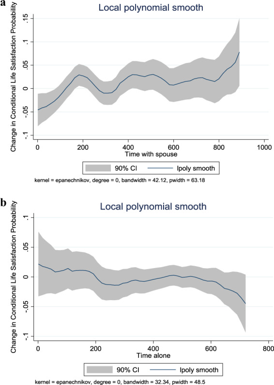
a Flexible estimates of the effect of time with spouse on the change in life satisfaction, married individuals without children, ATUS 2012–2013. b Flexible estimates of the effect of time alone on the change in life satisfaction, single individuals ages 30+ without children, ATUS 2012–2013

Robustness checks

Consider several re-specifications and sample restrictions. People who work in different industries may face different constraints on “who with” than others: e.g., educators may have more freedom to spend time with spouses. Also, people in different occupations (bank tellers) are more likely to have to work face-to-face during a pandemic; and alternatively, people in other occupations (economics researchers) may find tele-working easier.

To examine these potential difficulties, I re-estimate the models in Columns (1) and (4) of Table 2, adding indicators of industry (4-digit SIC) and occupation (4-digit SIC) to the equations. This is a more flexible way of examining the impacts of work that might be done more easily by tele-commuting or that might be viewed as essential than would be the arbitrary designation of certain industries/occupations as essential or as where tele-commuting is possible. The additions of these large vectors of indicators hardly change the estimated impacts of the “time with” variables. In the equation for childless married people the estimated coefficient on time with spouse declines slightly (to 0.0116, s.e. = 0.0049), as does the absolute value of the impact of time alone among singles (to −0.0103, s.e. = 0.0046).

In the sample of marrieds (singles), 1.9 (1.5)% of the diaries were collected on holidays, clearly atypical since the respondents’ choices about both time-use and “who with” are constrained to differ from non-holidays. Excluding these small fractions of respondents from the samples hardly changes the results. Roughly half the time diaries are kept on weekend days. “How” time is spent and “who with” differ between weekdays and weekends in both samples. Paid work is much less on weekends, as is well known, while time spent in all other aggregates of time use obviously increases. Married individuals spend more time with spouse and less time alone on weekends. Singles’ “who with” behavior varies less from weekday to weekend, except that they spend more time with friends on weekends. Despite these daily differences in “how” and “who with,” estimating the models underlying Table 2 separately for weekdays and weekends produces remarkably similar results to those shown in Table 2.13

One might also think that individuals whose leisure time includes more emailing off the job would be making different choices from those not spending (addicted to using) time in this way, since they are in contact with others even when alone. The models that include how people spend time, and their incomes, almost certainly already account for any effects of internet access on “who with” and how time is spent, as they control for the major determinants of internet access, income, education and age (Chaudhuri et al. 2005). Examining this issue by adding measures of daily time spent emailing for non-work purposes, however, barely alters the estimated impacts of choices about “who with” or “how” on satisfaction.

The estimates are all based on collapsing the life satisfaction measure into two categories—satisfied or not. To use all the information provided by the respondents in these ATUS modules, I re-estimate the equations shown in Table 2 using ordered probit analysis describing all 11 choices on the Cantril ladder. Re-estimating the model in Column (1) of Table 2 strengthens the results shown. The estimates on time with friends become statistically significantly positive, time with spouse remains statistically significantly positive and the overall vector of “who with” measures remains highly significant. Re-estimating the model in Column (4) of Table 2 yields similar inferences: time alone remains significantly negative, time with other relatives becomes significantly positive and the overall vector remains significant statistically. While in what follows I concentrate on the bivariate results for expositional and computational simplicity, one should note that they (very slightly) understate the statistical significance of the findings.

It is unlikely that reverse causation characterizes these estimates, as it is difficult to imagine that individuals who are inherently happier are those who choose to spend more time with spouse, or alone, or that they spend more time in paid work or home production. A reasonable concern, however, is that individuals who have been married longer become happier as a result and choose to spend more time with their spouse. The underlying effect may work through marital duration. The ATUS does not measure the duration of respondents’ marriages; but assuming, as the evidence shows, that most married individuals age 55+ have been married for many years, we can at least hint at the importance of this potential difficulty by restricting the married sample to the 70% of individuals age 55+.14 This reduction of the sample hardly changes the results: comparing the estimated impacts of “with spouse” to those shown in Column (1) of Table 2, the effect becomes 0.0191 (s.e. = 0.0053). This similarity suggests, but does not demonstrate, that this problem of selectivity is minor. There are numerous other factors that might alter the impacts of time use on satisfaction. But unless they are also (partially) correlated with “who with” or “how” or with income, they will not affect the estimated impacts of “how” and “who with” on satisfaction.15

A confirmation using British data

While the ATUS provides the largest data set on which to examine how people’s subjective well-being is affected by the identities of people within and outside their households with whom they spend time, the results depend entirely on how the underlying time diaries that respondents fill out are structured. The 2014–2015 UK. Time Use Survey provides a large cross-section of time diaries, with much of the same demographic information that accompanies the on-going ATUS, along with responses on a question about the individual’s life satisfaction. This is essentially the same question as in the 2012–2013 waves of the ATUS, but the responses are on a 7 to 1 scale. I define an indicator of satisfaction equaling 1 if the respondent answered 7 or 6 on this question, so that 2/3 of all respondents are coded as being satisfied, the closest approximation the dataset allows to the means calculated from the ATUS.

Because of the structure of the data, the sample of married couples includes childless couples and those with no young children (under age 8). The sample of singles ages 30+ is defined exactly as in the American data. Most of the respondents keep diaries and respond on their life satisfaction on two separate days. Unfortunately, it is not possible to disaggregate time spent with other (non-household relatives) and with friends or other people. There are thus three categories of “who with”: spouse, other people, or alone. Another major difference from the ATUS is that respondents may classify all 1440 min of the day by whom they are spent with (so that, for example, 7% of the sample of singles indicate that 1440 min are spent alone). Both samples are too small to allow useful comparisons by gender; but they are large enough to make it worthwhile to examine the models reported in Table 2 using the entire samples.

The estimates for the UK are shown in Table 4. Since most respondents provided information on their activities and satisfaction on two days, standard errors are clustered on individuals. All the underlying equations are specified as similarly as possible to their counterparts in Columns (1) and (4) of Table 2; and overall, the estimates are remarkably like those for the USA.

Table 4.

Estimates of the relation of different ways time is spent—alone and with others—to life satisfaction, men and women pooled, people without young children, UKTUS 2014–2015^a

	Married	Single ≥ 30
	(1)	(2)
Ind. Var. (in 100 min/day)
Alone	−0.0036 (0.0061)	−0.0076 (0.0054)
With other people	0.0118 (0.0058)	0.0091 (0.0070)
With spouse	0.0121 (0.0046)	–
p on F-statistic of “who with” vector	0.002	0.03
Adj. R2	0.182	0.284
N=	1870	1002

^aStandard errors in parentheses, clustered on individuals. Additional covariates included in the estimates: vectors of age indicators, years of educational attainment, region of residence, day of week, and month of year and household income, and the distribution of time spent on the diary day among work, home production, sleep, other personal care and TV-watching (with other leisure activities the excluded category)

Consider first married couples. As in the US data, additional time alone reduces a married person’s satisfaction, while more time with other people (which includes time with friends) increases it. The crucial result is that more time together with one’s spouse, other things equal, makes people significantly more satisfied. Even the marginal impact of additional time with spouse is near that shown in Table 2 (and in elasticity terms is almost identical). Finally, the vector of measures of “with whom” is jointly statistically significant. The results in the sample of singles also mirror those for the USA. As in that sample, additional time alone has a negative impact on subjective well-being, while time with other people has a positive impact.16 The point estimate of the effect of time alone is, however, smaller than in the US data.

Figure 2a, b shows respectively the results of local polynomial estimates of the impact of time with spouse on the life satisfaction of married respondents and of time spent alone on that of single individuals (because the data allow all time, not only non-sleep and non-personal time as in the ATUS, to be classified according to “who with,” the extreme value of 1440—the entire day—is not rare and makes sense). While the effects are not highly significantly nonlinear, there is some indication among the sample of married respondents that the positive marginal utility of time spent with one’s spouse/partner is diminishing, and, somewhat more weakly, that the marginal disutility of time spent alone by singles is also diminishing.

Fig. 2.

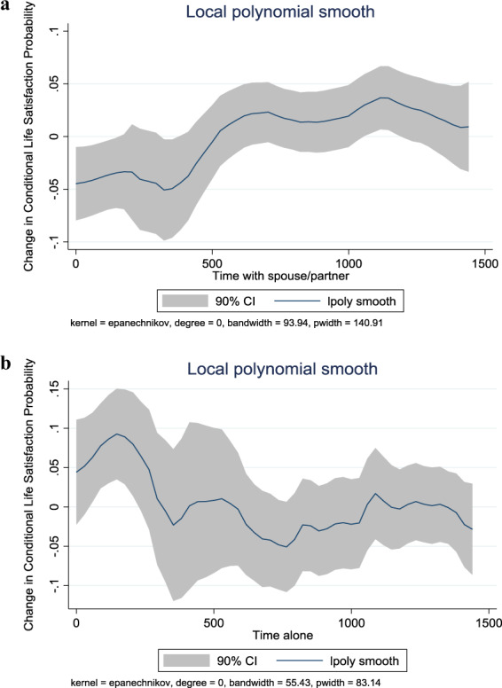
a Flexible estimates of the effect of time with spouse on the change in life satisfaction, married individuals without young children, UKTUS 2014–2015. b Flexible estimates of the effect of time alone on the change in life satisfaction, single individuals ages 30+ without young children, UKTUS 2014–2015

Simulating the impact of a lock-down on life satisfaction

With lock-downs people lose whatever freedom they had to maximize their satisfaction by choosing freely with whom they spend their time. Because they are confined to their residences during most of the day, they are limited to contact with many fewer people than if they could choose freely how to spend their time. Among married individuals with no children, I assume that a lock-down means that they spend much more time with their spouse. Among singles I assume that a lock-down increases their time remaining alone. While in both groups people might maintain electronic contacts with others, they have much less face-to-face contact with others.

I undertake three simulations using the results obtained from the ATUS, with all time listed “with whom” by married respondents re-classified to time with spouse, and among singles to time spent alone. The assumption underlying Simulation I is that there is no loss of work time and no loss of income. Those assumptions seem highly unrealistic. Many people lose jobs during a lock-down, and others see reductions in their work hours. In Simulation II I assume that 1/3 of work time is lost and is spent watching television. With the loss of work time, incomes almost certainly also drop. In Simulation III I assume that income also decreases in each sample by 1/3. Moving from Simulations I to II to III assumes increasingly negative effects of a lock-down on the real economy.

All these assumptions are arbitrary; we cannot know exactly by how much time with spouse increases among married couples, and by how much time alone increases among singles. Similarly, we cannot know exactly how much average work time decreases, although the biggest drop in the US (between February and April 2020) suggests, combining employment losses with hours of work of those remaining employed, that the decrease in work time was about 15%. The decline in real consumption spending over these two months was 19%.17 These data suggest that Simulations II and III generate upper-bound effects. In any case, since the impacts of time with spouse (time alone among singles) are nearly linear, the estimates are easily transformable using any arbitrary assumptions about changes in work time or spending.

The results of these simulations are shown in Table 5. Even with extreme assumptions about the extent of lost work time and income, among married individuals we see a substantial increase in the likelihood of reporting being satisfied with life. This is not true among singles: even under quite conservative assumptions (Simulation I), their satisfaction decreases; and with more extreme assumptions the decrease is substantial. Taken together, the most likely impacts are an increase in satisfaction among marrieds, a decrease in satisfaction among singles.

Table 5.

Simulations of the impact of changing time use during a lock-down, based on estimates in Columns (1) and (4) of Table 2 and Columns (2) and (4) of Table 3

Change in probability of being satisfied (≥8 life satisfaction)
Simulation	Married, no children	Single ≥ 30, no children
	(1)	(2)
I. Changes in “who with”
Reported time shifted to spouse (alone)	0.081	−0.034
II. Adds 1/3 cut in work time, shifted to TV-watching
Reported time shifted to spouse (alone)	0.063	−0.047
III. Adds 1/3 cut in income
Reported time shifted to spouse (alone)	0.043	−0.059

The effect of a lock-down on the well-being of different groups might differ for reasons other than the “who with” or “how” of time use. Work time and income losses clearly are not homogeneous across the population, and similarly for the risk of contracting and dying from an illness that induces the lock-down (Borjas 2020). Results might differ between majority and minority citizens for these reasons. All I have shown is that average married couple’s well-being might increase because of a lock-down per se, while that of the average single individual would be reduced.

I stress that these simulations ignore any change in well-being, presumably negative, that would result from insecurities and other fears associated with a pandemic. All they show is that, because married people enjoy being with their spouses, spending still more time with them per se increases their life satisfaction. Similarly, because additional time spent alone reduces the life satisfaction of single people, a lockdown that increases their time alone per se reduces their life satisfaction.

Conclusions and implications

The results here use two years of data from the American Time Use Survey to demonstrate that, after adjusting for numerous covariates including the activities on which people spend their time, the identities of people with whom they associate affect their expressed life satisfaction. I use similar data from the UK to estimate the same models. Whether these implied marginal utilities decrease in absolute value is unclear: there is no sign of any decrease in the US data, but there is some in the UK data.

I use the US results to simulate the impact of massive increases in time spent with one’s spouse (among married couples) and alone (among singles) resulting from lock-downs. These simulations mimic the likely impacts of Covid-19 related lock-downs. They suggest that for married couples, whatever decline in satisfaction is generated by the lack of freedom and by uncertainty about income and life generally is at least partly mitigated by spending more time with one’s spouse. Among singles the opposite is the case: any generalized reduction in satisfaction is exacerbated by the additional time that they must spend alone.

The simulations rely on the underlying notion that utility depends not only on goods and services purchased and time spent, but also upon the identities of with whom, if anyone, the time is spent. Assuming that people choose along these three dimensions, how can it be, ignoring generalized dissatisfaction caused by uncertainties resulting from a pandemic, that married people could be better off when they cannot make these choices freely because they are locked down? A possible explanation is that when not locked down they are not totally free to choose “who with,” because their favorite choice—their spouse—is for most of them unavailable during time spent in paid work, a major component of the representative day. With lock-downs married individuals are constrained to spend more time with their most utility-enhancing person. The constraint might reduce the well-being of singles compared to the unconstrained situation, because it imposes more work time alone, their most utility-reducing “who with” choice.

Compliance with ethical standards

Conflict of interest

The author declares no conflict of interest.

References

- Abraham K, Maitland A, Bianchi S. Non-response in the American Time Use Survey. Public Opinion Quarterly. 2006;70(5):676–703. doi: 10.1093/poq/nfl037. [DOI] [Google Scholar]
- Becker G. A theory of the allocation of time. Economic Journal. 1965;75(299):493–517. doi: 10.2307/2228949. [DOI] [Google Scholar]
- Blanchflower, D., & Oswald, A. (2017). Do humans suffer a psychological low in midlife? Two approaches (with and without controls) in seven data sets. NBER Working Paper No. 23724.
- Borjas G. Demographic determinants of testing incidence and COVID-19 infections in New York City neighborhoods. Covid Economics. 2020;3:12–39. [Google Scholar]
- Chaudhuri A, Flamm K, Horrigan J. An analysis of the determinants of internet access. Telecommunications Policy. 2005;29:731–755. doi: 10.1016/j.telpol.2005.07.001. [DOI] [Google Scholar]
- Connelly R, Kimmel J. If you’re happy and you know it: how do mothers and fathers in the US really feel about caring for their children? Feminist Economics. 2015;21(1):1–34. doi: 10.1080/13545701.2014.970210. [DOI] [Google Scholar]
- Diener, E., Kahneman, D. & Helliwell, J. (2010). International differences in well-being. Oxford University Press, New York.
- Easterlin R. Income and happiness: towards a unified theory. Economic Journal. 2001;111(473):465–484. doi: 10.1111/1468-0297.00646. [DOI] [Google Scholar]
- Flood S, Genadek K. Time for each other: work and family constraints among couples. Journal of Marriage and the Family. 2016;78(1):142–164. doi: 10.1111/jomf.12255. [DOI] [PMC free article] [PubMed] [Google Scholar]
- Gimenez-Nadal JI, Molina JA. Voluntary activities and daily happiness in the United States. Economic Inquiry. 2015;53(4):1735–1750. doi: 10.1111/ecin.12227. [DOI] [Google Scholar]
- Hallberg D. Synchronous leisure, jointness and household labor supply. Labour Economics. 2003;10(2):185–203. doi: 10.1016/S0927-5371(03)00006-X. [DOI] [Google Scholar]
- Hamermesh D. Timing, togetherness and time windfalls. Journal of Population Economics. 2002;15(4):601–623. doi: 10.1007/s001480100092. [DOI] [Google Scholar]
- Hamermesh, D. (2019). Spending time: the most valuable resource. Oxford University Press, New York.
- Hamermesh D, Frazis H, Stewart J. Data watch: the American Time Use Survey. Journal of Economic Perspectives. 2005;19(1):221–232. doi: 10.1257/0895330053148029. [DOI] [Google Scholar]
- Hofferth S, Flood S, Sobek M. American time use survey data extract builder: version 2.7 [dataset] MN: University of Maryland and Minneapolis; 2018. [Google Scholar]
- Kahneman D, Krueger A, Schkade D, Schwarz N, Stone A. A survey method for characterizing daily life experience: the day reconstruction method. Science. 2004;306(5702):1776–1780. doi: 10.1126/science.1103572. [DOI] [PubMed] [Google Scholar]
- Knabe A, Rätzel S, Schöb R, Weimann J. Dissatisfied with life but having a good day: time-use and well-being of the unemployed. Economic Journal. 2010;120(547):867–889. doi: 10.1111/j.1468-0297.2009.02347.x. [DOI] [Google Scholar]
- Michaud P-C, Vermeulen F. A collective labor supply model with complementarities in leisure: identification and estimation by means of panel data. Labour Economics. 2011;18(2):159–167. doi: 10.1016/j.labeco.2010.10.005. [DOI] [Google Scholar]
- Pollak R. Interdependent preferences. American Economic Review. 1976;66(3):309–320. [Google Scholar]
- Stone A, Schneider S, Krueger A, Schwartz J, Deaton A. Experiential wellbeing data from the American Time Use Survey: comparisons with other methods and analytic illustrations with age and income. Social Indicators Research. 2018;136(1):359–378. doi: 10.1007/s11205-016-1532-x. [DOI] [PMC free article] [PubMed] [Google Scholar]