

Abstract
In this work, we formulate and analyze a new mathematical model for COVID-19 epidemic with isolated class in fractional order. This model is described by a system of fractional-order differential equations model and includes five classes, namely, S (susceptible class), E (exposed class), I (infected class), Q (isolated class), and R (recovered class). Dynamics and numerical approximations for the proposed fractional-order model are studied. Firstly, positivity and boundedness of the model are established. Secondly, the basic reproduction number of the model is calculated by using the next generation matrix approach. Then, asymptotic stability of the model is investigated. Lastly, we apply the adaptive predictor–corrector algorithm and fourth-order Runge–Kutta (RK4) method to simulate the proposed model. Consequently, a set of numerical simulations are performed to support the validity of the theoretical results. The numerical simulations indicate that there is a good agreement between theoretical results and numerical ones.
Keywords: COVID-19 epidemic, Stability analysis, Adaptive predictor–corrector algorithm, Fractional differential equations, Numerical simulations
Introduction
Mathematical models describing infectious diseases have an important role both in theory and practice (see, for example, [6–8, 18, 34]). The construction and analysis of models of this type can help us understand the mechanism of the transmission as well as characteristics of diseases, and therefore, we can propose effective strategies to predict, prevent, and restrain diseases, as well as to protect population health. Up to now, many mathematical models for infectious diseases formulated by differential equations have been constructed and analyzed to study the spreading of viruses, for instance, [6–8, 18, 34]. Recently, mathematical models for COVID-19 epidemic have attracted the attention of many mathematicians, biologists, epidemiologists, pharmacists, chemists with many notable and important results (see, for instance, [1, 5, 9, 14, 15, 19, 23, 26, 28–30, 33, 35, 36] and references therein). This can be considered an effective approach to study, simulate, and predict the mechanism and transmission of COVID-19.
Motivated by the above reason, in this work, we formulate and analyze a new mathematical model for COVID-19 epidemic. This model is described by a system of fractional-order differential equations model and includes five classes, namely, S (susceptible class), E (exposed class), I (infected class), Q (isolated class), and R (recovered class). This model is a generalization of a well-known ODE model formulated in [35]. In the proposed fractional-order model, we use the Caputo fractional derivative instead of the integer-order one because when modeling processes and phenomena arising in the real world, fractional-order models are more accurate than integer-order ones. In particular, fractional-order models provide more degrees of freedom in the model while an unlimited memory is also guaranteed in contrast to integer-models with limited memory [11, 24, 27].
Our main aim is to study the dynamics and numerical approximations for the proposed fractional-order model. Firstly, the positivity and boundedness of the model are investigated based on standard techniques of mathematical analysis. Secondly, the basic reproduction number of the model is calculated by using the next generation matrix approach. Then, asymptotic stability of the model is investigated based on the Lyapunov stability theorem for fractional dynamical systems. Lastly, we apply the adaptive predictor–corrector algorithm and fourth-order Runge–Kutta (RK4) method formulated in [20] to simulate the proposed model. Consequently, a set of numerical simulations is performed to support the validity of the theoretical results. The numerical simulations indicate that there is a good agreement between theoretical results and numerical ones.
This work is organized as follows. The fractional-order differential model is formulated in Sect. 2. Dynamics of the model is investigated in Sect. 3. Numerical simulations by the adaptive predictor–corrector algorithm are performed in Sect. 4. The last section present some remarks, conclusions, and discussions.
Model formulation
The total population is divided into five compartments: susceptible (S), exposed (E), infected (I), isolated (Q), and recovered (R) from the disease. We assume that all the classes are normalized. This leads to the mathematical model formulation in which the interaction of the exposed population and infected population is linked to the susceptible population. In this model, we assume that the natural death rate includes the disease death rate. When there is no symptom of the disease, the exposed class moves with a certain rate to the isolated class, but in the case when symptoms are developed, it moves to the infected class. Keeping in mind the above assumptions, we obtain the following ODE model (see [35]):
| 1 |
where the parameters and variables used are described in Table 1.
Table 1.
Parameters in the model
| Symbols | Description |
|---|---|
| S | Susceptible population |
| E | Exposed population |
| I | Infected Population |
| Q | Isolated population |
| R | Recovered population |
| Λ = μN | Recruitment rate |
| β | Rate at which susceptible move to infected and exposed class |
| π | Rate at which exposed population moves to infected one |
| γ | Rate at which exposed people become isolated |
| σ | Rate at which infected people are added to isolated individuals |
| θ | Rate at which isolated persons become recovered |
| μ | Natural death rate plus disease related death rate |
Let us introduce the notation
| 2 |
From the ODE system (1), we obtain
which implies that the total population in this case we take as constant because .
To include into the model (1) the past history or hereditary properties, we replace the first derivative by the Caputo fractional derivative. More precisely, we propose the following system of fractional differential equations:
| 3 |
where , and denotes the fractional derivative in the Caputo sense. We refer the readers to [2–4, 10, 25] for the definition of the fractional Caputo derivative.
Dynamics of the fractional-order model
Positivity and boundedness
Let us denote
The following theorem is proved by using a generalized mean value theorem [21, 22] and a fractional comparison principle [16, Lemma 10].
Theorem 1
(Positivity and boundedness)
Let be any initial data belonging to and be the solution corresponding to the initial data. Then, the set is a positively invariant set of the model (3). Furthermore, we have
| 4 |
Proof
First, it is easy to prove the existence and unique of solutions of the model thanks to results proved in [17].
For the model (3), we have
| 5 |
By (5) and the generalized mean value theorem [21, 22], we deduce that for all .
From the first equation of the system (3), we obtain
By using the fractional comparison principle, we have the first estimate of (4).
From the second equation of the system (3), we have
which implies that
Consequently, we have the second estimate of (4).
From the third equation of the system (3), we get
for t large enough. This implies the third estimate of (4).
From the fourth equation of the system (3), we have
for t large enough. From this we get the fourth estimate of (4).
Finally, the fifth equation of (3) implies that
which implies the fifth estimate of (4). The proof is complete. □
Equilibria and the reproduction number
Firstly, to find equilibria of the model (3), we consider the following algebraic system:
| 6 |
By some algebraic manipulations, we obtain two solutions of the system (6) that are
| 7 |
and
| 8 |
Note that , , , and are positive if and only if
We now compute the reproduction number of the model (3) by using the next generation matrix approach developed by van den Driessche and Watmough [31]. Let . We rewrite the model (3) in the matrix form
| 9 |
where
| 10 |
Hence, the reproduction number of the model (3) can be determined by
| 11 |
It is easy to verify that , , , , and if and only if .
Theorem 2
(Equilibria)
The model (3) always possesses a disease-free equilibrium (DFE) point given by (8) for all values of the parameters. Moreover, the model has a unique disease endemic equilibrium point given by (9) if and only if .
Stability analysis
Theorem 3
The DFE point of the model (3) is locally asymptotically stable if .
Proof
The Jacobian matrix of the model (3) at the DFE point is
| 12 |
The characteristic polynomial of J is
where
| 13 |
It is easy to verify that if , then and . This implies that two roots of the polynomial have negative real parts. Consequently, the real parts of five eigenvalues of the matrix are all negative, or equivalently, is locally stable. The proof is complete. □
We now prove the uniform asymptotical stability of the DFE point of the model (3) by using the Lyapunov stability theorem [12, Theorem 3.1].
Theorem 4
If , then the DFE point of the model (3) is not only locally asymptotically stable but also uniformly asymptotically stable.
Proof
Since the first three equations of the model (3) do not depend on the states Q and R, we need only consider the following subsystem:
| 14 |
From (4), it is sufficient to consider the model (3) in its feasible set defined by
Consider a Lyapunov function given by
| 15 |
By using the linearity property of the Caputo derivative and [32, Lemma 3.1] and some algebraic manipulations, we obtain
where
It is easy to check that if , then . Consequently, by the Lyapunov stability theorem for fractional dynamical systems, we deduce that is uniformly asymptotically stable. The proof is complete. □
Remark 1
The analysis of stability of is an interesting mathematical problem, but in this work, we mainly focus on the case to find an effective strategy to prevent the disease.
sensitivity analysis
Theorem 3 suggests that we should control the parameters such that . This provides a good strategy to prevent and restrain the disease. More precisely, when , then
which means that the disease will be completely controlled and prevented. Motivated by this, we now perform an sensitivity analysis to find ways to choose suitable parameters.
It is easy to verify that
| 16 |
Equation (16) suggests some ways to choose the parameters such that . Hence, based on this, we can propose suitable strategies to control and prevent the disease.
Numerical simulations by the adaptive predictor–corrector algorithm
The adaptive predictor–corrector algorithm
In this section we review the method that is proposed by [20]. The proposed algorithm is given as follows. Consider the initial value problem (IVP) governed by:
| 17 |
where is the proposed generalized Caputo-type fractional derivative operator given [20, Definition 4]. Initially, for , , and , the IVP (17) is equivalent, using [20, Theorem 3], to the Volterra integral equation:
| 18 |
where
| 19 |
The first step of our algorithm, under the assumption that the function f is such that a unique solution exists on some interval , consists of dividing the interval into N unequal subintervals , using the mesh points
| 20 |
where . Now, we are going to generate the approximations , , to solve numerically the IVP (17). The basic step, assuming that we have already evaluated the approximations (), is that we want to get the approximation by means of the integral equation
| 21 |
Making the substitution
| 22 |
we get
| 23 |
that is,
| 24 |
Next, if we use the trapezoidal quadrature rule with respect to the weight function to approximate the integrals appear in the right-hand side of Eq. (24), replacing the function by its piecewise linear interpolant with nodes chosen at the (), then we obtain
| 25 |
Thus, substituting the above approximations into Eq. (24), we obtain the corrector formula for , ,
| 26 |
where
| 27 |
The last step of our algorithm is to replace the quantity shown on the right-hand side of formula (26) with the predictor value that can be obtained by applying the one-step Adams–Bashforth method to the integral equation (23). In this case, by replacing the function with the quantity at each integral in Eq. (24), we get
| 28 |
Therefore, the present adaptive predictor–corrector algorithm, for evaluating the approximation , is completely described by the formula
| 29 |
where , , and the predicted value can be determined as described in Eq. (28) with the weights being defined according to (27). It is easily observed that when , the present adaptive predictor–corrector algorithm will be reduced to the predictor–corrector approach presented in [13].
Implementation with numerical simulation
In this section, we solve numerically Eq. (3) using the method given in the former section. In view of the above algorithm, following the rule (27), the approximations , , , , and can be simply evaluated using the iterative formulas, for and ,
where and
Parameter values which are calculated for basic time of coronavirus used in numerical example are ; ; ; ; ; ; , with total population and initial data .
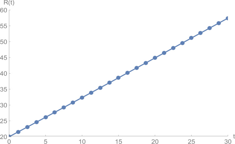
In Figs. 1–5, we plot numerical solutions of the model (3) with obtained using the proposed algorithm and the RK4 method when and for . From the graphical results in Figs. 1–5, it can be seen that the results obtained using the proposed algorithm match the results of the RK4 method very well, which implies that the presented method can predict the behavior of these variables accurately in the region under consideration.
Figure 2.
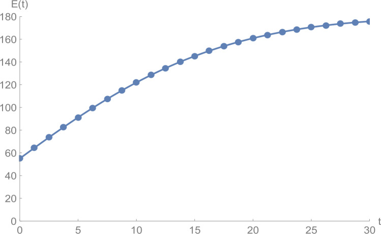
versus t: solid line presents the proposed approximation, dotted line stands for RK4 method
Figure 3.
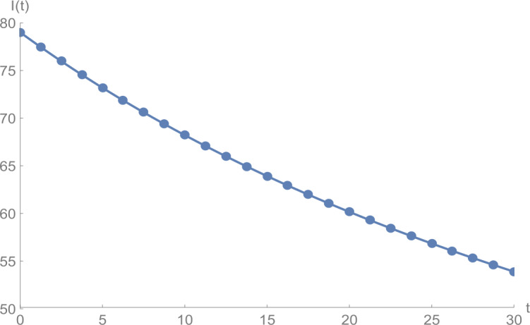
against t: solid line presents the proposed approximation, dotted line stands for RK4 method
Figure 4.
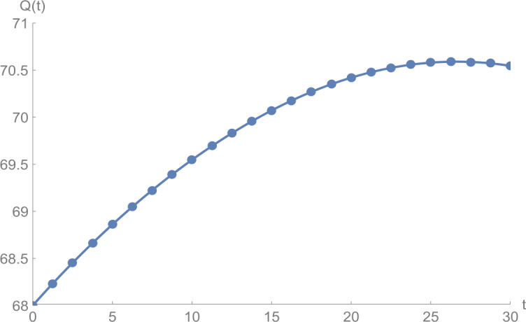
against t: solid line presents the proposed approximation, dotted line stands for RK4 method
Figure 1.
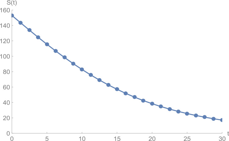
against t: solid line presents the proposed approximation, dotted line stands for RK4 method
Figure 5.
against t: solid line presents the proposed approximation, dotted line stands for RK4 method
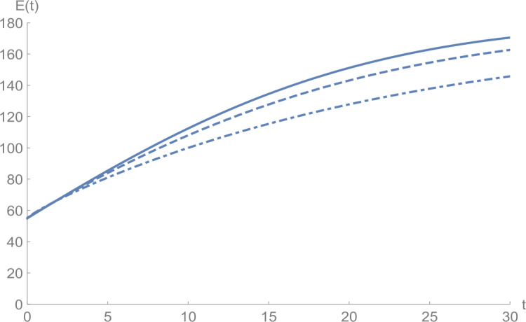
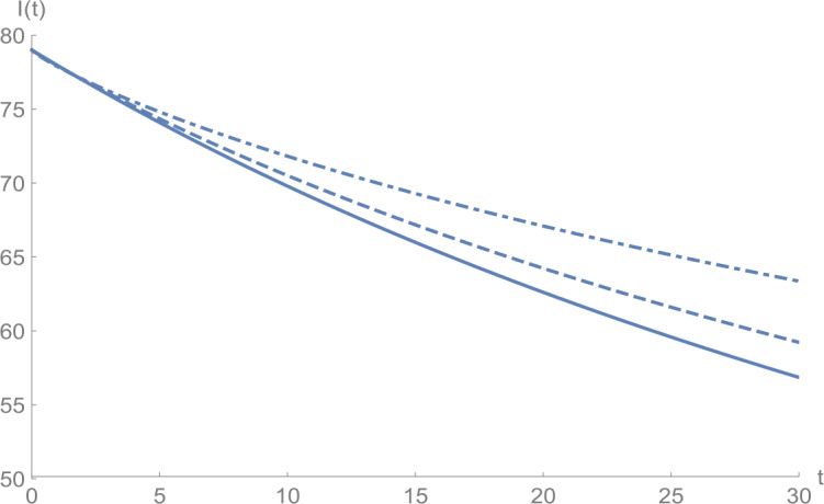
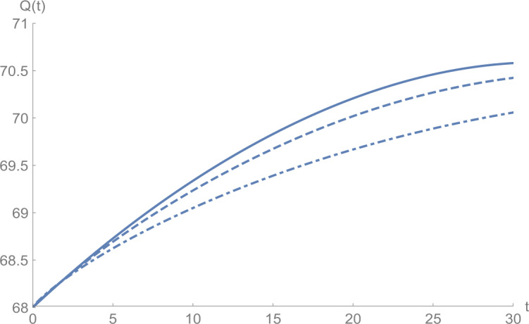
Figures 6–10 show the approximate solutions for , , , , and obtained for different values of α using the proposed algorithm. From the graphical results given in Figs. 6–10, it is clear that the approximate solutions depend continuously on the time-fractional derivative α. It is evident that the efficiency of this approach can be dramatically enhanced by decreasing the step size.
Figure 7.
against t: (solid line) , (dot-dashed line) , (dashed line)
Figure 8.
against t: (solid line) , (dot-dashed line) , (dashed line)
Figure 9.
against t: (solid line) , (dot-dashed line) , (dashed line)
Figure 6.
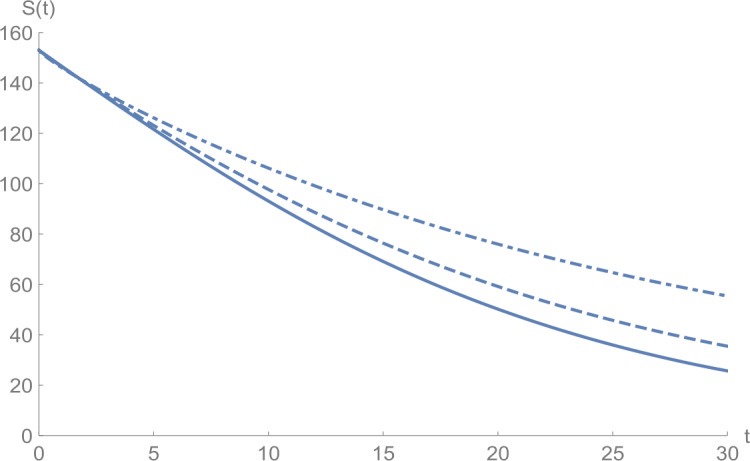
against t: (solid line) , (dot-dashed line) , (dashed line)
Figure 10.
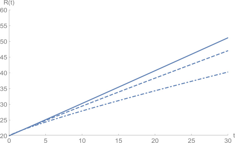
against t: (solid line) , (dot-dashed line) , (dashed line)
Remarks and conclusions
In this paper, we have formulated and analyzed a new mathematical model for COVID-19 epidemic. The model is described by a system of fractional-order differential equations and includes five classes, namely, S (susceptible class), E (exposed class), I (infected class), Q (isolated class), and R (recovered class). It should be emphasized that the model is a generalization of our recent work proposed in [35].
Firstly, the positivity, boundedness, and stability of the model have been established. Furthermore, the basic reproduction number of the model has been calculated by using the next generation matrix approach. Lastly, we have applied the adaptive predictor–corrector algorithm and fourth-order Runge–Kutta (RK4) method to simulate the proposed model. A set of numerical simulations has been performed to support the validity of the theoretical results. The numerical simulations indicate that there is a good agreement between theoretical results and numerical ones.
In the near future, we will extend the results in this work to propose new mathematical models for COVID-19 epidemic. Especially, effective strategies to control and prevent the disease will be investigated.
Acknowledgments
Acknowledgements
The authors thank the editor and anonymous referees for useful comments that led to a great improvement of the paper.
Availability of data and materials
The authors confirm that the data supporting the findings of this study are available within the article cited herein.
Authors’ contributions
Authors have equally contributed in preparing this manuscript. All authors read and approved the final manuscript.
Funding
This paper was supported by the Natural Science Foundation of the Higher Education Institutions of Anhui Province (No. KJ2020A0002).
Competing interests
The authors declare that there is no conflict of interest regarding the publication of this paper.
Contributor Information
Zizhen Zhang, Email: zzzhaida@163.com.
Anwar Zeb, Email: anwar@cuiatd.edu.pk.
Oluwaseun Francis Egbelowo, Email: oluwaseun@aims.edu.gh.
Vedat Suat Erturk, Email: vserturk@omu.edu.tr.
References
- 1.Abdo M.S., Hanan K.S., Satish A.W., Pancha K. On a comprehensive model of the novel coronavirus (COVID-19) under Mittag-Leffler derivative. Chaos Solitons Fractals. 2020;135:109867. doi: 10.1016/j.chaos.2020.109867. [DOI] [PMC free article] [PubMed] [Google Scholar]
- 2.Atangana A. Fractal-fractional differentiation and integration: connecting fractal calculus and fractional calculus to predict complex system. Chaos Solitons Fractals. 2017;102:396–406. doi: 10.1016/j.chaos.2017.04.027. [DOI] [Google Scholar]
- 3.Atangana A. Blind in a commutative world: simple illustrations with functions and chaotic attractors. Chaos Solitons Fractals. 2018;114:347–363. doi: 10.1016/j.chaos.2018.07.022. [DOI] [Google Scholar]
- 4.Atangana A. Fractional discretization: the African’s tortoise walk. Chaos Solitons Fractals. 2020;130:109399. doi: 10.1016/j.chaos.2019.109399. [DOI] [Google Scholar]
- 5.Bekiros S., Kouloumpou D. SBDiEM: a new mathematical model of infectious disease dynamics. Chaos Solitons Fractals. 2020;136:109828. doi: 10.1016/j.chaos.2020.109828. [DOI] [PMC free article] [PubMed] [Google Scholar]
- 6.Bocharov G., Volpert V., Ludewig B., Meyerhans A. Mathematical Immunology of Virus Infections. Berlin: Springer; 2018. [Google Scholar]
- 7.Brauer F. Mathematical epidemiology: past, present, and future. Infect. Dis. Model. 2017;2:113–127. doi: 10.1016/j.idm.2017.02.001. [DOI] [PMC free article] [PubMed] [Google Scholar]
- 8.Brauer F., van den Driessche P., Wu J. Mathematical Epidemiology. Berlin: Springer; 2008. [Google Scholar]
- 9.Cakan S. Dynamic analysis of a mathematical model with health care capacity for COVID-19 pandemic. Chaos Solitons Fractals. 2020;139:110033. doi: 10.1016/j.chaos.2020.110033. [DOI] [PMC free article] [PubMed] [Google Scholar]
- 10.Caputo M. Linear models of dissipation whose Q is almost frequency independent-II. Geophys. J. Int. 1967;13(5):529–539. doi: 10.1111/j.1365-246X.1967.tb02303.x. [DOI] [Google Scholar]
- 11.Daftardar-Gejji V. Fractional Calculus and Fractional Differential Equations. Basel: Birkhäuser; 2019. [Google Scholar]
- 12.Delavari H., Baleanu D., Sadati J. Stability analysis of Caputo fractional-order nonlinear systems revisited. Nonlinear Dyn. 2012;67:2433–2439. doi: 10.1007/s11071-011-0157-5. [DOI] [Google Scholar]
- 13.Diethelm K., Ford N., Freed A. A predictor–corrector approach for the numerical solution of fractional differential equations. Nonlinear Dyn. 2002;29:3–22. doi: 10.1023/A:1016592219341. [DOI] [Google Scholar]
- 14.Higazy M. Novel fractional order SIDARTHE mathematical model of COVID-19 pandemic. Chaos Solitons Fractals. 2020;138:110007. doi: 10.1016/j.chaos.2020.110007. [DOI] [PMC free article] [PubMed] [Google Scholar]
- 15.Kumar S., Cao J., Abdel-Aty M. A novel mathematical approach of COVID-19 with non-singular fractional derivative. Chaos Solitons Fractals. 2020;139:110048. doi: 10.1016/j.chaos.2020.110048. [DOI] [PMC free article] [PubMed] [Google Scholar]
- 16.Li Y., Cheng Y., Podlubny I. Mittag-Leffler stability of fractional order nonlinear dynamic systems. Automatica. 2009;45:1965–1969. doi: 10.1016/j.automatica.2009.04.003. [DOI] [Google Scholar]
- 17.Lin W. Global existence theory and chaos control of fractional differential equations. J. Math. Anal. Appl. 2007;332(1):709–726. doi: 10.1016/j.jmaa.2006.10.040. [DOI] [Google Scholar]
- 18.Martcheva M. An Introduction to Mathematical Epidemiology. New York: Springer; 2015. [Google Scholar]
- 19. Ming, W., Huang, J.V., Zhang, C.J.P.: Breaking down of the healthcare system: mathematical modelling for controlling the novel coronavirus (2019-nCoV) outbreak in Wuhan, China (2020). 10.1101/2020.01.27.922443
- 20.Odibat Z., Baleanu D. Numerical simulation of initial value problems with generalized Caputo-type fractional derivatives. Appl. Numer. Math. 2020;156:94–110. doi: 10.1016/j.apnum.2020.04.015. [DOI] [Google Scholar]
- 21.Odibat Z., Baleanu D. Numerical simulation of initial value problems with generalized Caputo-type fractional derivatives. Appl. Numer. Math. 2020;156:94–105. doi: 10.1016/j.apnum.2020.04.015. [DOI] [Google Scholar]
- 22.Odibat Z., Shawagfeh N. Generalized Taylor’s formula. Appl. Math. Comput. 2007;186(1):286–293. doi: 10.1016/j.amc.2006.07.102. [DOI] [Google Scholar]
- 23.Okuonghae D., Omame A. Analysis of a mathematical model for COVID-19 population dynamics in Lagos, Nigeria. Chaos Solitons Fractals. 2020;139:110032. doi: 10.1016/j.chaos.2020.110032. [DOI] [PMC free article] [PubMed] [Google Scholar]
- 24.Oldham K., Spanier J. The Fractional Calculus Theory and Applications of Differentiation and Integration to Arbitrary Order. Amsterdam: Elsevier; 1974. [Google Scholar]
- 25.Podlubny I. Fractional Differential Equations. San Diego: Academic Press; 1998. [Google Scholar]
- 26.Postnikov E.B. Estimation of COVID-19 dynamics “on a back-of-envelope”: does the simplest SIR model provide quantitative parameters and predictions? Chaos Solitons Fractals. 2020;135:109841. doi: 10.1016/j.chaos.2020.109841. [DOI] [PMC free article] [PubMed] [Google Scholar]
- 27.Samko S.G., Kilbas A.A., Mariuchev O.I. Fractional Integrals and Derivatives. Milton Park: Taylor & Francis; 1993. [Google Scholar]
- 28.Shah K., Abdeljawad T., Mahariq I., Jarad F. Qualitative analysis of a mathematical model in the time of COVID-19. BioMed Res. Int. 2020;2020:5098598. doi: 10.1155/2020/5098598. [DOI] [PMC free article] [PubMed] [Google Scholar]
- 29.Torrealba-Rodriguez O., Conde-Gutiérrez R.A., Hernández-Javiera A.L. Modeling and prediction of COVID-19 in Mexico applying mathematical and computational models. Chaos Solitons Fractals. 2020;138:109946. doi: 10.1016/j.chaos.2020.109946. [DOI] [PMC free article] [PubMed] [Google Scholar]
- 30.Ud Din R., Shah K., Ahmad I., Abdeljawad T. Study of transmission dynamics of novel COVID-19 by using mathematical model. Adv. Differ. Equ. 2020;2020:323. doi: 10.1186/s13662-020-02783-x. [DOI] [PMC free article] [PubMed] [Google Scholar]
- 31.van den Driessche P., Watmough J. Reproduction numbers and sub-threshold endemic equilibria for compartmental models of disease transmission. Math. Biosci. 2002;180:29–48. doi: 10.1016/S0025-5564(02)00108-6. [DOI] [PubMed] [Google Scholar]
- 32.Vargas-De-Leon C. Volterra-type Lyapunov functions for fractional-order epidemic systems. Commun. Nonlinear Sci. Numer. Simul. 2015;24:75–85. doi: 10.1016/j.cnsns.2014.12.013. [DOI] [Google Scholar]
- 33.Yousaf M., Muhammad S.Z., Muhammad R.S., Shah H.K. Statistical analysis of forecasting COVID-19 for upcoming month in Pakistan. Chaos Solitons Fractals. 2020;138:109926. doi: 10.1016/j.chaos.2020.109926. [DOI] [PMC free article] [PubMed] [Google Scholar]
- 34.Zaman G., Jung H., Torres D.F.M., Zeb A. Mathematical modeling and control of infectious diseases. Comput. Math. Methods Med. 2017;2017:7149154. doi: 10.1155/2017/7149154. [DOI] [PMC free article] [PubMed] [Google Scholar]
- 35.Zeb A., Alzahrani E., Erturk V.S., Zaman G. Mathematical model for coronavirus disease 2019 (COVID-19) containing isolation class. BioMed Res. Int. 2020;2020:3452402. doi: 10.1155/2020/3452402. [DOI] [PMC free article] [PubMed] [Google Scholar]
- 36.Zhang Z. A novel COVID-19 mathematical model with fractional derivatives: singular and nonsingular kernels. Chaos Solitons Fractals. 2020;139:110060. doi: 10.1016/j.chaos.2020.110060. [DOI] [PMC free article] [PubMed] [Google Scholar]
Associated Data
This section collects any data citations, data availability statements, or supplementary materials included in this article.
Data Availability Statement
The authors confirm that the data supporting the findings of this study are available within the article cited herein.