Modeling surface water dynamics in the Amazon Basin using MOSART-Inundation-v1.0: Impacts of geomorphological parameters and river flow representation

Abstract

Surface water dynamics play an important role in water, energy and carbon cycles of the Amazon Basin. A macro-scale inundation scheme was integrated with a surface-water transport model and the extended model was applied in this vast basin. We addressed the challenges of improving basin-wide geomorphological parameters and river flow representation for large-scale applications. Vegetation-caused biases embedded in the HydroSHEDS DEM data were alleviated by using a vegetation height map of about 1-km resolution and a land cover dataset of about 90-m resolution. The average elevation deduction from the DEM correction was about 13.2 m for the entire basin. Basin-wide empirical formulae for channel cross-sectional geometry were adjusted based on local information for the major portion of the basin, which could significantly reduce the cross-sectional area for the channels of some subregions. The Manning roughness coefficient of the channel varied with the channel depth to reflect the general rule that the relative importance of riverbed resistance in river flow declined with the increase of river size. The entire basin was discretized into 5395 subbasins (with an average area of 1091.7 km²), which were used as computation units. The model was driven by runoff estimates of 14 years (1994 – 2007) generated by the ISBA land surface model. The simulated results were evaluated against in situ streamflow records, and remotely sensed Envisat altimetry data and GIEMS inundation data. The hydrographs were reproduced fairly well for the majority of 13 major stream gauges. For the 11 subbasins containing or close to 11 of the 13 gauges, the timing of river stage fluctuations was captured; for most of the 11 subbasins, the magnitude of river stage fluctuations was represented well. The inundation estimates were comparable to the GIEMS observations. Sensitivity analyses demonstrated that refining floodplain topography, channel morphology and Manning roughness coefficients, as well as accounting for backwater effects could evidently affect local and upstream inundation, which consequently affected flood waves and inundation of the downstream area. It was also shown that the river stage was sensitive to local channel morphology and Manning roughness coefficients, as well as backwater effects. The understanding obtained in this study could be helpful to improving modeling of surface hydrology in basins with evident inundation, especially at regional or larger scales.

1. Introduction

The terrestrial surface water dynamics have significant impacts on the water, energy and carbon cycles of the planet, as they influence energy and material exchange between the land surface and the atmosphere. For instance, surface water bodies are important natural sources of greenhouse gases (e.g., carbon dioxide and methane) (Bousquet et al., 2006; Richey et al., 2002). Extreme events such as river inundation have extraordinary effects on the land surface – groundwater interactions and the sediment and nutrient exchange between rivers and floodplains, and thereby influence land and aquatic ecosystems as well as their feedback to the atmosphere. Therefore, improving parameterizations of surface water dynamics is meaningful in studying the linkages between the land surface and climate.

Many previous studies of surface-hydrology modeling were conducted for the Amazon River which is the largest river of the globe and accounts for about 18% of the total continental freshwater discharge to oceans (Dai and Trenberth, 2002). Seasonal floods occur every year and wetlands occupy a considerable proportion of the total area in this basin (Hess et al., 2003, 2015). River and inundation dynamics were simulated by using 2-D hydrodynamic models at the central Amazonia (e.g., Baugh et al., 2013; Wilson et al., 2007). Using fine-resolution grid cells (e.g., ~ 300 m) as computation units, 2-D hydrodynamic models could represent water flow over floodplains. They were not applied at regional or larger scales due to computational costs. On the other hand, some computationally efficient macro-scale inundation schemes were used in a few continental-scale hydrologic models for the entire Amazon Basin (e.g., Coe et al., 2008; Decharme et al., 2008; Getirana et al., 2012; de Paiva et al., 2013; Vörösmarty et al., 1989; Yamazaki et al., 2011). While those models with macro-scale inundation schemes could capture some aspects of surface water dynamics fairly well, a number of challenges have been identified, including uncertainties in model inputs of floodplain and channel morphology, flow parameterization for gentle-gradient river reaches, etc.

Topography data are essential inputs in hydrologic modeling. At present the common practice is to use the digital elevation model (DEM) to represent topography. Because the coverage of high-accuracy DEM data (e.g., with elevation errors less than 1 m) is limited, hydrologic modeling at regional or larger scales uses DEM data obtained by spaceborne sensors. The Shuttle Radar Topography Mission (SRTM) DEM data have been widely used for hydrologic modeling, but some factors limit their accuracy. In forested regions such as the Amazon Basin, primary biases in SRTM DEM data were caused by vegetation cover because the radar signal was not able to penetrate the vegetation canopy (Sanders, 2007). Previous studies in the Amazon Basin adopted various approaches to alleviate the vegetation-caused biases embedded in SRTM data. In some modeling studies, elevation values were lowered by a constant in forested area of the entire basin, ignoring the spatial variability of vegetation heights (e.g., Coe et al., 2008; de Paiva et al., 2013). In a few hydrodynamic modeling studies for the central Amazonia, the vegetation-caused biases in SRTM elevations were derived from spatially varied vegetation heights. For example, Wilson et al. (2007) estimated the vegetation-height distribution based on their field survey of various vegetation types and a map of vegetation types (Hess et al., 2003); Baugh et al. (2013) utilized a global dataset of spatially distributed vegetation heights developed by Simard et al. (2011).

Channel cross-sectional geometry affects the estimation of channel flow velocity and channel storage capacity in the modeling of surface water dynamics. Distributed hydrologic modeling at regional or larger scales needs cross-sectional dimensions of all the channels that constitute the river network in the study domain. Channel cross-sectional dimensions obtained from in situ measurements are reliable, but limited to a small number of locations. Therefore channel cross-sectional dimensions were usually estimated based on available basin characteristics by using empirical formulae. Modeling studies in the Amazon Basin employed relationships between channel geometry and streamflow statistics (Getirana et al., 2012; Yamazaki et al., 2011) or upstream drainage area (Beighley et al., 2009; Coe et al., 2008; de Paiva et al., 2013) (those relationships are also referred to as “channel geometry formulae” in this article). In most of these studies, cross-sectional geometry of all the channels spread over the Amazon Basin were estimated by using one set of channel geometry formulae and corresponding parameters, which represented average characteristics of the entire basin. So for different subregions of the basin, channel cross-sectional dimensions derived from the same formulae and parameters contained biases of various magnitudes. Hydrologic modeling results were demonstrated to be sensitive to channel cross-sectional dimensions (e.g., Getirana et al., 2013; Yamazaki et al., 2011) so improving the channel dimensions to be more representative of the actual channel morphology could be important.

The Manning formula has been used for estimating flow velocities of rivers in many continental- or global-scale hydrologic models. In this formula, the Manning roughness coefficient (also abbreviated to “Manning coefficient” hereinafter; in this article, the “Manning roughness coefficient” discussed is for river channels) is a key and sensitive parameter (de Paiva et al., 2013; Yamazaki et al., 2011) which, however, can only be estimated empirically. In previous studies of the Amazon Basin, the Manning coefficient was determined using various approaches: (a) a constant value for the entire basin (Beighley et al., 2009; Yamazaki et al., 2011); (b) different values for different subregions calibrated using hydrographs at stream-gauge locations of major rivers (de Paiva et al., 2013); (c) diverse values dependent on the channel cross-sectional dimensions that vary spatially (Getirana et al., 2012, 2013). For natural river channels, the Manning coefficient depends on many factors, including riverbed roughness, cross-sectional geometry and channel sinuosity (Arcement and Schneider, 1989). The significant variations of these factors within a basin undermine the rationale of a uniform Manning coefficient across the entire basin or a few Manning coefficients for different subregions of the basin. The aforementioned approach (c) reflects the general phenomenon that the relative importance of riverbed friction in river flow becomes smaller for larger rivers. This approach can represent the major aspect of the spatial variation of Manning coefficients.

The Amazonia is characterized by flat gradients and backwater effects are evident in river flows (Meade et al., 1991). Trigg et al. (2009) analyzed the characteristics of flood waves and conducted hydraulic modeling for reaches of the central Amazonia. They demonstrated that it was necessary to account for backwater effects and the diffusion wave method was valid for modeling the Amazon flood waves. The backwater effects were also represented in some continental-scale models applied in this basin. Yamazaki et al. (2011) used both the kinematic wave and diffusion wave methods to simulate river flow, with the latter capable of simulating backwater effects. Paiva et al. (2013) used the full Saint-Venant equations (or the dynamic wave method) to represent water flow of river reaches with gentle riverbed slope and large floodplains. These studies showed that accounting for backwater effects could evidently improve the modeling of surface water dynamics in this basin.

In this study, a surface-water transport model was extended with a macro-scale inundation scheme, and the extended model was applied in the Amazon Basin. Efforts were made to refine model geomorphological parameter inputs, which have important effects on inundation but are difficult to determine for basin-scale simulations. We focused specifically on floodplain topography and channel cross-sectional geometry. The vegetation-caused biases in the DEM data were estimated based on spatially varied vegetation heights for the entire Amazon Basin. The channel geometry biases were alleviated by adjusting the basin-wide channel geometry formulae for different subregions based on channel morphology information of local locations. We also aimed to improve the river flow representation and its parameters. The Manning roughness coefficient depended on the river size and its spatial variation was represented. The diffusion wave method was chosen to model river flow in channels and the backwater effects were accounted for.

The model performance was evaluated against gauged streamflow data, as well as river-stage and inundation data obtained by satellites. Sensitivity analyses were conducted to investigate the impacts of improving floodplain topography, channel morphology, and Manning roughness coefficients, as well as accounting for backwater effects on surface water dynamics.

2. Methods and data

2.1. Surface-water transport model

The Model for Scale Adaptive River Transport (MOSART) was developed to simulate terrestrial surface water flow from hillslopes to the basin outlet (Li et al., 2013). Two simplified forms of the one-dimensional Saint-Venant equations (i.e., kinematic wave or diffusion wave methods) are used to represent water flow over hillslopes, in minor tributaries (named as tributary subnetwork), or in major channels. The MOSART model is driven by runoff estimates from the land surface model. Surface runoff is treated as input of overland flow, which is represented with the kinematic wave method and enters the tributary subnetwork, while subsurface runoff directly enters the tributary subnetwork. Water flow in the tributary subnetwork is also represented with the kinematic wave method and the outflow finds its way to the major channel (or main channel). Either the diffusion wave method or kinematic wave method could be used to simulate water flow in main channels. The two methods use the same continuity equation, and differ in the momentum equation and Manning’s equation.

In the diffusion wave method, the momentum equation is expressed as (Chow et al., 1988):

$$g\frac{\partial y}{\partial x}-g{S}_0+g{S}_f=0$$ (1)

where is the gravitational acceleration [unit: m s⁻²]; y is the water depth in the channel [unit: m]; x is the distance along the river [unit: m]; S₀ is the riverbed slope [dimensionless] and S_f is the friction slope [dimensionless], which could be positive or negative. $g\frac{\partial y}{\partial x}$ is the pressure force term, gS₀ is the gravity force term and gS_f is the friction force term.

The Manning’s equation is expressed as:

$$v=\frac{S_f}{\left|S_f\right|}{n}^{-1}{R}^{\frac{2}{3}}{\left|S_f\right|}^{\frac{1}{2}}$$ (2)

where n is the Manning roughness coefficient [unit: s · m^−1/3] and R is the hydraulic radius [unit: m].

The continuity equation, momentum equation and Manning’s equation are combined to determine the flow velocity, channel water depth and friction slope. The friction slope depends on water depth variation along the channel so it is affected by the river stage of the downstream channel. This way, backwater effects are represented. One extreme phenomenon caused by backwater effects is that when the downstream river stage is higher than the river stage of the current channel and hence S_f is negative, the flow velocity from Eq. (2) is also negative, so water flows from downstream to upstream.

In the kinematic wave method, the pressure force term is neglected from the momentum equation. With this simplification, the friction slope equals the riverbed slope and backwater effects are not represented.

2.2. Macro-scale inundation scheme

In this study the MOSART model was extended with a macro-scale inundation scheme and the extended model was named “MOSART-Inundation”. River inundation dynamics was represented by macro-scale inundation schemes in a few previous studies (Coe et al., 2008; Decharme et al., 2008; Getirana et al., 2012; de Paiva et al., 2013; Yamazaki et al., 2011). Those studies used relatively coarse computation units with the area magnitude ranging from 100 to 10,000 km². The main feature of their macro-scale inundation schemes was that the water level–inundated area relationship for the computation unit was used to estimate flood extent. The inundation scheme of this study is similar to those of Yamazaki et al. (2011) and Getirana et al. (2012). In this scheme, each computation unit (a squared grid or a subbasin) has a main channel and a floodplain reservoir (Fig. 1a). Flooding water can spill out of the main channel and enter the floodplain reservoir, or recede from the floodplain reservoir to the main channel. The water storage within each computation unit is used with a water stage versus flooded area curve (referred to as “elevation profile”) to estimate the flooded area within the unit. The elevation profile is derived from DEM data within the computation unit (Fig. 1b). The channel–floodplain exchange is assumed to be instantaneous for each time step (i.e., the channel stage and the floodplain stage are level at the end of each time step).

Figure 1.

Illustrations of the macro-scale inundation scheme: (a) Illustration of river overflow; (b) Elevation profiles of a computation unit (e.g., a grid cell or subbasin). The brown solid line is the original elevation profile. The green dash line is the amended elevation profile (its non-channel part overlaps with the original elevation profile). A_c is the fraction of the channel area in the computation unit.

The channel area is implicitly included in an elevation profile, which is developed from all the elevations of the fine-resolution DEM within the computation unit (Fig. 1b: the brown solid line). Getirana et al. (2012) proposed an amended elevation profile in which the channel area was distinguished from the non-channel area. Their method was adopted in this study. It is assumed that the main channel consists of the lowest pixels of the DEM within a computation unit. So the main channel and the rest of the computation unit (including the floodplain) are represented by the lower part and the upper part of the elevation profile, respectively. The dividing point corresponds to the fraction of channel area, which is estimated as the product of the channel length derived from DEM data and the channel width calculated with empirical formulae (Sect. 2.5). The elevation of the dividing point corresponds to the channel bank top. If the channel cross-sectional shape is assumed to be a rectangle, the channel part of the elevation profile changes to be the green dash line in Fig. 1b: when the river stage is lower than the bank top, the water surface area does not change with the river stage and always equals the channel area. As the river stage exceeds the bank top, the total water storage is used with the amended elevation profile to estimate the total water surface area (including the channel area and the flooded area in the floodplain).

2.3. Application in the Amazon Basin

The MOSART-Inundation model was applied to the entire Amazon Basin. The study domain of 5.89 million km² was divided into 5395 subbasins (the average area is 1091.7 km² and the standard deviation is 921.5 km²), which were used as computation units (Figs. 2a and 2b). Each subbasin has a main channel and the entire river network consists of 5395 main channels (Fig. 2a).

Figure 2.

Basin discretization and model inputs. (a) The river network extracted from the DEM overlaps with 13 stream gauges: a) Altamira; b) Itaituba; c) Fazenda vista alegre; d) Canutama; e) Gaviao; f) Acanaui; g) Serrinha; h) Cach da porteira-con; i) Santo antonio do ica; j) Itapeua; k) Manacapuru; l) Jatuarana+Careiro; m) Obidos. (b) Magnified quadrat. The thin (thick) black lines mark boundaries between subbasins (subregions). (c) Delineation of 10 subregions (including 9 tributary subregions and the mainstem subregion indicated by dark green color). (d) Average DEM deduction for each subbasin to alleviate vegetation-caused biases. (e) The corrected DEM. (f) Averaged elevation profiles based on the original and corrected DEMs. (g) Channel widths. (h) Channel depths. (i) Manning roughness coefficients of channels.

In order to analyze the spatially varied characteristics of inundation results, the Amazon Basin was also divided into 10 subregions (Fig. 2c). Twenty eight major-tributary catchments were first delineated and some neighboring major-tributary catchments were combined so the 28 catchments were aggregated to 9 tributary subregions. All the minor tributary catchments and the area draining directly to the mainstem were aggregated to be the mainstem subregion.

The inputs of surface and subsurface runoff, which were of 1-degree resolution, were produced by the ISBA land surface model (Getirana et al., 2014) driven by the ORE-HYBAM precipitation dataset (Guimberteau et al., 2012). The grid based runoff data were converted to subbasin based runoff data using area-weighted averaging method for driving the simulations of this study.

The inputs of DEM data, channel cross-sectional geometry and Manning roughness coefficients, as well as the setup of simulations are described in the following subsections.

2.4. Vegetation-caused biases in DEM

The 3-second resolution HydroSHEDS DEM data developed by United States Geological Survey (USGS) (http://hydrosheds.cr.usgs.gov/) were used in this study. The HydroSHEDS DEM data included void-filled DEM data and hydrologically conditioned DEM data. The conditioned DEM was used to generate the digital river network and subbasins, and the void-filled DEM was used to generate the elevation profiles of all the subbasins.

The conditioned DEM was not suitable for representing floodplain topography and generating elevation profiles. In the DEM conditioning process, the elevation values of pixels for river channels and their buffer zones were lowered by non-negligible amounts that could be larger than 20 m in the lower mainstem area of the Amazon Basin. So the channels and their adjacent areas in the conditioned DEM could hold more water than the actual counterparts, which would lead to underestimation of flood extent.

The HydroSHEDS DEM data were derived from the SRTM data and inherited the vegetation-caused biases. Before being used for producing elevation profiles, the void-filled HydroSHEDS DEM was processed to alleviate the biases caused by vegetation. The vegetation height data with ~ 1-km resolution developed by Simard et al. (2011) was used. For vegetated areas, the original void-filled DEM represented elevations of locations within the vegetation canopy. So, part of the vegetation height needed to be deducted from the original elevation. Baugh et al. (2013) found that deducting 50 – 60% of the vegetation height of the Simard et al. (2011) data from the original DEM achieved the greatest improvements to hydrodynamic model accuracy in the Amazon floodplain. A deduction ratio of 50% was used for the vegetated area in this study.

The resolution of the vegetation height data was coarser than that of the DEM data. It might not be appropriate to assume a uniform vegetation height for all the DEM pixels within the grid cell of the vegetation height dataset. Hess et al. (2003, 2015) developed a high resolution (3 arc seconds) land cover dataset for floodplains (or wetlands) located in the lowland Amazon Basin (i.e., areas with elevations lower than 500 m). This land cover dataset was used in our DEM correction process. In the floodplains of the lowland Amazon Basin, vegetation height removal was conducted differently for different land cover classes. For DEM pixels with forest or woodland classes, 50% of the vegetation height was deducted from the original DEM. In the high resolution land cover dataset, shrubs were defined to be less than 5 m tall (Junk et al., 2011). If the vegetation height was larger than 5 m for DEM pixels with shrub, the vegetation height was reduced to be 5 m. Therefore, for shrub DEM pixels with vegetation heights equal to or higher than 5 m, the elevations were lowered by 2.5 m, but if the vegetation heights were less than 5 m, the elevations were lowered by 50% of the vegetation heights. For DEM pixels with other land cover classes (e.g., open water, bare soil, etc.), the elevations were not modified. For areas outside of the floodplains of the lowland basin, a uniform vegetation height was applied for all the DEM pixels that overlap with the vegetation height pixel. This approximation was not expected to have obvious effects on inundation modeling since most inundation occurred within the floodplains of the lowland basin.

The DEM correction obviously changed the topographic features in the DEM data. The average elevation deduction in each subbasin ranges from 0 to 21 m (Fig. 2d). After the DEM correction, the average elevation in each subbasin ranges from 0 to 4772 m (Fig. 2e). For all the subbasins, the ratio of the average elevation deduction to the subbasin elevation difference (i.e., the difference between the highest and lowest elevations in the subbasin) ranges from 0 to 52.9% (average: 9.2%; standard deviation: 7.1%). The average elevation profile of the Amazon Basin was generated for the original DEM and corrected DEM, respectively (Fig. 2f). At first, the normalized elevation profile was produced for each subbasin. For each DEM pixel within a subbasin, the elevation relative to the lowest pixel of the subbasin was divided by the subbasin elevation difference to give the normalized elevation, which was used to generate the normalized elevation profile. Then the normalized elevation profiles of all subbasins were averaged to give the average elevation profile of the entire basin. Figure 2f illustrates that the DEM processing evidently lowers the average elevation profile.

2.5. Channel cross-sectional geometry

At regional or larger scales, channel cross-sectional shape is usually simplified to be a rectangle since the channel top width is much larger than the channel depth (or bank height). The channel cross-section can be determined by channel width and channel depth. Beighley and Gummadi (2011) presented a methodology for estimating channel cross-sectional dimensions (i.e., channel width and channel depth) at stream-gauge locations by using stage – discharge relationship data and Landsat imagery. They implemented the approach to derive channel cross-sectional dimensions of 82 streamflow gauging locations spread over the Amazon Basin, which were further used to develop the general relationships between channel cross-sectional dimensions and upstream drainage area (or channel geometry formulae) for the entire basin. Their channel geometry formulae are listed as follows.

$$w=1.956A^{0.413}\left(A<10,000k{m}^2\right)$$ (3)

$$w=0.403A^{0.600}\left(A\ge 10,000k{m}^2\right)$$ (4)

$$d=0.245A^{0.342}$$ (5)

where w is channel width (unit: m); d is channel depth (unit: m); A is upstream drainage area (unit: km²). Beighley and Gummadi (2011) showed that the channel cross-sectional dimensions estimated from their channel geometry formulae agreed well with those from the formulae by Coe et al. (2008). Based on extensive river morphology data obtained from stations spread throughout the Amazon and Tocantins basins, Coe et al. (2008) derived the general channel geometry formulae for the Amazon Basin and, in their formulae, channel cross-sectional dimensions were also expressed as power functions of upstream drainage area.

The channel geometry formulae of Beighley and Gummadi (2011) were obtained through regression analysis of data from 82 locations over the Amazon Basin, and reflected the average feature of the basin. Directly applying the same formulae and parameters to the entire basin could cause large biases in the estimated channel cross-sectional dimensions for some subregions. In order to reduce those biases, in this study the coefficients in the basin-wide channel geometry formulae of Beighley and Gummadi (2011) were adjusted for a majority of the 10 subregions (Fig. 2c) based on channel cross-sectional dimensions of local locations. The 82 streamflow gauging locations scattered over the Amazon Basin and each subregion contained a few streamflow gauging locations. For the streamflow gauging locations of the same subregion, the root-mean-square error (RMSE) between the channel cross-sectional dimensions estimated with the channel geometry formulae and the corresponding dimensions presented in Beighley and Gummadi (2011) could be calculated. During the adjustment process, the coefficient of the channel geometry formula (i.e., 1.956, 0.403 or 0.245 in Eqs. (3)–(5)) was multiplied by a factor to reduce the RMSE. The factor values for the 10 subregions are listed in Table 1. The ranges for the channel width and depth of each subbasin are shown in Figs. 2g and 2h, respectively.

Table 1.

Coefficients in channel geometry formulae for the subregions.

No.	Subregion name	Factor for adjusting channel width (αw)	Channel width coefficient		Factor for adjusting channel depth (αd)	Channel depth coefficient	Factor for adjusting cross-sectional area (αw = αw·αd)
			Au < 10000 km2	Au ≥ 10000 km2
1	Xingu	1.0	1.956	0.403	1.0	0.245	1.00
2	Tapajos	1.6	3.130	0.645	0.7	0.172	1.12
3	Madeira	0.6	1.174	0.242	0.6	0.147	0.36
4	Purus	0.8	1.565	0.322	1.4	0.343	1.12
5	Jurua	0.7	1.369	0.282	1.5	0.368	1.05
6	Upper-Solimoes tributaries	1.0	1.956	0.403	1.0	0.245	1.00
7	Japura	1.8	3.521	0.725	0.7	0.172	1.26
8	Negro	1.7	3.325	0.685	0.5	0.123	0.85
9	Northeast	0.6	1.174	0.242	0.8	0.196	0.48
10	Mainstem	1.0	1.956	0.403	1.0	0.245	1.00

Note: A_u is upstream drainage area.

It is worth mentioning that Paiva et al. (2013) also accounted for spatial variability of channel geometry formulae and used various coefficients in their formulae for six zones of the Amazon Basin. In this study, we used both the basin-wide channel geometry formulae and the diverse formulae for various subregions, and investigated the effects of adjusting channel geometry on modeled surface water dynamics.

2.6. Manning roughness coefficients for channels

The Manning roughness coefficient for channels reflects the resistance to water flows in channels and is determined by many factors, such as roughness of riverbed and riverbank, shape and size of channel cross-sections and channel meanderings. In general, within a basin these factors have considerable spatial heterogeneities. Therefore it is more reasonable to use spatially varied coefficients estimated based on these factors than using a constant coefficient. However, distributed hydrologic modeling requires channel Manning coefficient value for each subbasin, which is not realistic given the lack of information. For continental- or global-scale studies, the river network consists of river channels of distinct magnitude orders. Riverbed resistance plays a relatively smaller role in water flows of larger channels. Assuming that the Manning coefficient decreases linearly with the channel top width, Decharme et al. (2010) showed that the assumed relationship produced acceptable variation in flow velocity in a global application of the ISBA-TRIP continental hydrological modeling system. Getirana et al. (2012) expressed the Manning coefficient as a power function of the channel depth in their study of inundation dynamics in the Amazon Basin. In this study, the Manning coefficient also depended on the channel depth and was estimated using the following function:

$$n=n_{\text{min}}+\left(n_{\text{max}}-n_{\text{min}}\right)\left(\frac{h_{\text{max}}-h}{h_{\text{max}}-h_{\text{min}}}\right)$$ (6)

where the maximum Manning coefficient n_max is for the channel with the shallowest channel depth and the minimum Manning coefficient n_min is for the channel with the largest channel depth. n_max and n_min were set as 0.05 and 0.03, respectively, based on the literature. h_max and h_min are the maximum and minimum channel depths in all the channels, and were estimated to be 50.64 and 0.96 m, respectively, using the method described in the previous subsection. The variable h is the depth of the current channel. The spatial distribution of the channel Manning coefficient is shown in Fig. 2i.

The function of the Manning coefficient (i.e., Eq. (6)) was compared to those of Decharme et al. (2010) and Getirana et al. (2012) in this study. In general, compared to the equations of the two previous studies, Eq. (6) gave smaller Manning coefficients and resulted in better simulated hydrographs, which suggested that Eq. (6) was more appropriate for the simulations of this study.

2.7. Setup of simulations

Five simulations were conducted in this study (Table 2). The first simulation used the optimal combination of the four factors (i.e., DEM, channel cross-sectional geometry, Manning roughness coefficients and the parameterization for channel water flow) and was set as the control simulation (abbreviated as CTL). For the purpose of investigating the effects of each of the four factors on surface water dynamics, only one factor was changed in each of the other four simulations. In the second simulation, the original HydroSHEDS DEM data without the correction of vegetation-caused biases were used; in the third simulation, the basin-wide channel geometry formulae were not adjusted for the subregions and were directly used for the entire basin; in the fourth simulation, the spatially varied Manning roughness coefficients for channels were replaced with a constant coefficient of 0.03; lastly the diffusion wave method was replaced by the kinematic wave method for representing water flow through channels in the fifth simulation. All simulations were run for 14 years (1994 – 2007) and the results of 13 years (1995 – 2007) were analyzed. The results of the control simulation were used in model evaluation and the results of all simulations were utilized for sensitivity analysis.

Table 2.

Setup of simulations.

No.	Method for representing river flow	DEM	Manning roughness coefficients of channels	Channel cross-sectional geometry	Abbreviations
1	Diffusion wave method	Corrected	Varied	Adjusted	CTL
2	Diffusion wave method	Original	Varied	Adjusted	OriDEM
3	Diffusion wave method	Corrected	Varied	No adjusting	OriSec
4	Diffusion wave method	Corrected	0.03	Adjusted	n003
5	Kinematic wave method	Corrected	Varied	Adjusted	KW

3. Model evaluation

3.1. Streamflow

The observed daily streamflow data for model evaluation were from 13 stream gauges operated by the Brazilian Water Agency. Eight of the 13 gauges either control the major area of a tributary subregion or are typical gauges in their tributary subregions. None of the 13 gauges is located in the tributary subregion “Upper-Solimoes tributaries” in the western Amazon Basin. Streamflow of this subregion can be approximately represented by that of the Santo antonio do ica gauge at the upper mainstem. The remaining four gauges are along the middle or lower mainstem.

The simulated daily streamflow results were compared with the observed data for a 12-year period (1995 – 2006) at the 13 stream gauges (Fig. 3). The Nash–Sutcliffe efficiency coefficient (NSE) and the relative error of mean annual streamflow (RE) were calculated for each gauge (Fig. 3). For the majority of the 13 gauges, daily streamflow values were reproduced fairly well. The NSE value is higher than 0.62 at seven gauges. The four gauges with NSE values lower than 0.5 have high absolute values of RE (i.e., > 0.20), which suggests that large biases in runoff inputs for the areas upstream of those gauges degrade the streamflow results. Overall, runoff inputs have large negative biases in the western portion of the Amazon Basin, and large positive biases in the southern and southeastern portions.

Figure 3.

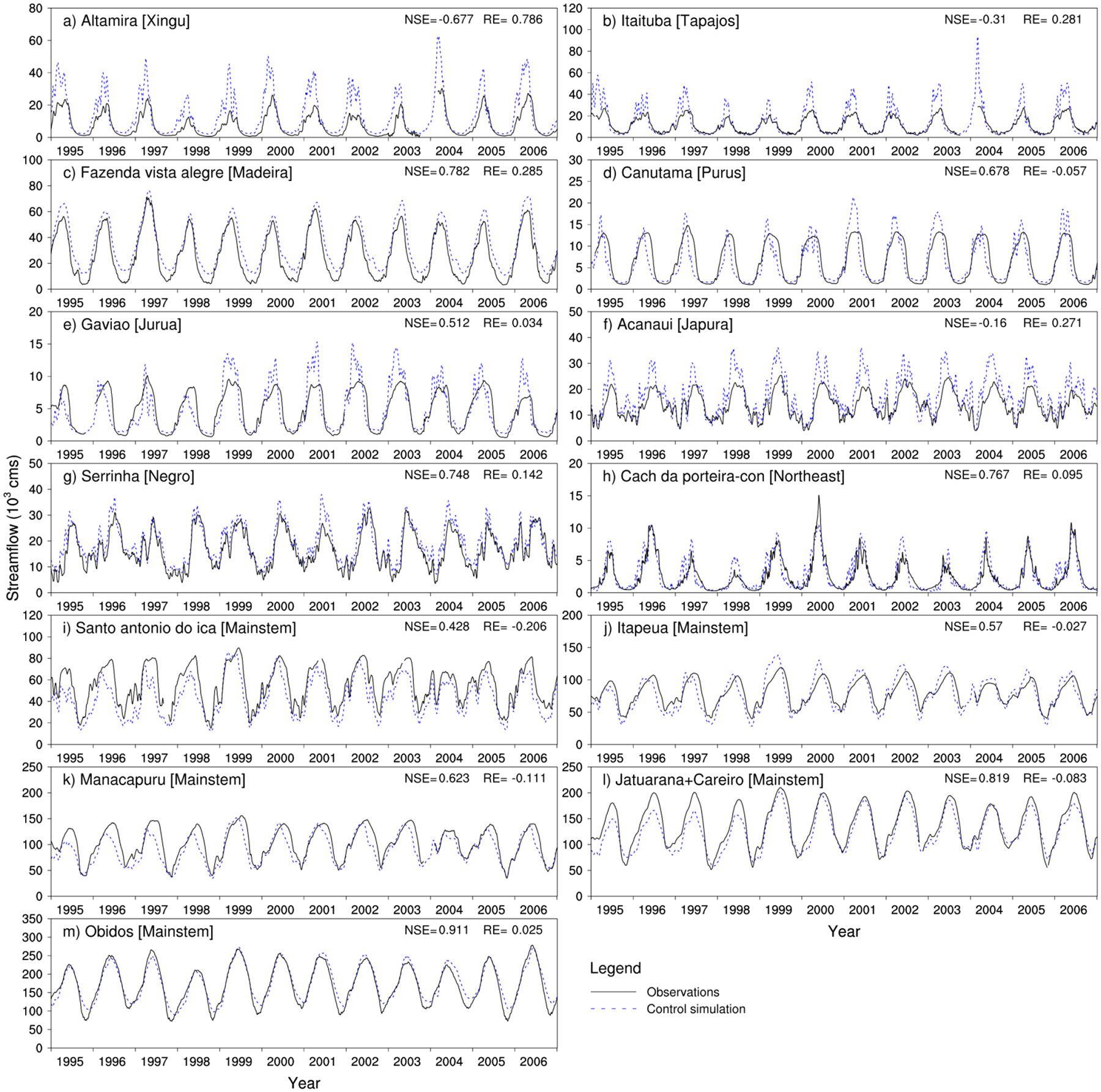
Comparison between modeled and observed daily streamflow for a 12-year period (1995 – 2006) at 13 stream gauges (the corresponding subregion names are shown in the brackets): a) Altamira [Xingu]; b) Itaituba [Tapajos]; c) Fazenda vista alegre [Madeira]; d) Canutama [Purus]; e) Gaviao [Jurua]; f) Acanaui [Japura]; g) Serrinha [Negro]; h) Cach da porteira-con [Northeast]; i) Santo antonio do ica [Mainstem]; j) Itapeua [Mainstem]; k) Manacapuru [Mainstem]; l) Jatuarana+Careiro [Mainstem]; m) Obidos [Mainstem]. The Nash–Sutcliffe efficiency coefficient and the relative error of mean annual streamflow are indicated at the upper right corner of each panel. Figure 2a shows the stream-gauge locations.

3.2. River stage

The observed river stages were based on altimetry data obtained by the Envisat satellite. The altimetry data were stored in the Hydroweb server (http://ctoh.legos.obs-mip.fr/products/hydroweb). This study utilizes river stages of 11 virtual stations which correspond to 11 of the 13 stream gauges used in Sect. 3.1. Each of the 11 virtual stations is close to one gauge: the virtual station and the gauge are located in either the same subbasin or two neighboring subbasins. There is no virtual station close to the Altamira or Cach da porteira-con gauges.

The simulated river stages are relative elevations as they were calculated from the riverbed elevation and the channel water depth. The riverbed elevation was estimated by using the following equation since observed data were not available.

$$E_c=E_{\mathit{\text{mouth}}}+\sum _{i=1}^n{L}_i{S}_i+\frac{1}{2}{L}_c{S}_c$$ (7)

where E_c is the average riverbed elevation of the current channel [unit: m]; E_mouth is the riverbed elevation at the mouth of the Amazon River [unit: m]; n is the total number of the downstream channels; L_i is the flow length of one downstream channel i [unit: m]; S_i is the average riverbed slope of one downstream channel i [dimensionless]; L_c is the flow length of the current channel [unit: m] and S_c is the average riverbed slope of the current channel [dimensionless]. Considerable uncertainties in the riverbed elevation are expected due to the large uncertainties in the riverbed elevation at the mouth (E_mouth) and the riverbed slope. Therefore the simulated river stage of a channel is negatively affected by parameter biases of downstream channels and cannot be directly compared to the observations.

The timing and magnitude of simulated river stage fluctuations were compared to those of observed data. The comparison was conducted at the daily scale during a 6-year period (2002 – 2007) for the 11 subbasins which contained the 11 virtual stations (Fig. 4). For better visual comparison, the simulated river stages were shifted to coincide with the observations. The Pearson correlation coefficient between the simulated river stages and the observed data, as well as standard deviation for simulated and observed river stages were calculated. The timing of the simulated river stage fluctuations is in good agreement with the observations in all 11 subbasins, with Pearson correlation coefficients ranging from 0.830 to 0.960. The river stage fluctuations are captured well in the majority of the 11 subbasins, and overestimated for the subbasins of 4 gauges (i.e., Canutama, Acanaui, Serrinha and Santo antonio do ica): the standard deviation of the simulated river stages is much larger than that of the observed data, which could be primarily due to a few reasons: (1) overestimation of streamflow peaks (e.g., Canutama and Acanaui), which could be caused by biases of runoff inputs or underestimation of flood extent in the upstream area; (2) uncertainties in model parameters of channel cross-sectional geometry, channel Manning coefficients, etc.

Figure 4.

Comparison of modeled daily river stages with the observations for a 6-year period (2002 – 2007) at the subbasins containing or close to 11 of the 13 stream gauges (the corresponding subregion names are shown in the brackets): a) Itaituba [Tapajos]; b) Fazenda vista alegre [Madeira]; c) Canutama [Purus]; d) Gaviao [Jurua]; e) Acanaui [Japura]; f) Serrinha [Negro]; g) Santo antonio do ica [Mainstem]; h) Itapeua [Mainstem]; i) Manacapuru [Mainstem]; j) Jatuarana+Careiro [Mainstem]; k) Obidos [Mainstem]. The Pearson correlation coefficient between modeled river stages and the observations, as well as standard deviation for modeled and observed river stages, are indicated in each panel. The simulated river stages are shifted to coincide with the observations for better visual comparison (please see the Sect. 3.2 for the detailed explanation).

3.3. Flood extent

The simulated flood extent results were evaluated using the Global Inundation Extent from Multi-Satellite (GIEMS) data (Papa et al., 2010; Prigent et al., 2007, 2012). The GIEMS data contained monthly surface water area during a 15-year period (1993 – 2007) for each of the land pixels of equal area (i.e., 773 km²). The area-weighted averaging method was used to convert the grid based surface water extent data to subbasin based data for using in this study. Lake area was not deducted from the GIEMS data because in the Amazon Basin the lakes usually were located in the low portion of one subbasin and the simulated inundated area also contained lake area.

The simulated monthly flood extent results (including channel surface area and flooded area over floodplains) were compared to the GIEMS data during a 13-year period (1995 – 2007) for 10 subregions and the entire Amazon Basin (Fig. 5). The Pearson correlation coefficient and the mean annual relative difference between the simulated flood extent results and the observations were calculated. The timing of inundation was reproduced well for most area of the Amazon Basin: the Pearson correlation coefficient is equal to or larger than 0.727 at seven of the ten subregions and the entire basin. The mean annual value of simulated flood extent is comparable to that of the GIEMS observations for major portion of the basin: the absolute value of the mean annual relative difference is less than 0.23 at seven of the ten subregions and the entire basin.

Figure 5.

Comparison of modeled monthly flood extent to the GIEMS satellite observations during a 13-year period (1995 – 2007) for 10 subregions and the entire Amazon Basin: a) Xingu; b) Tapajos; c) Madeira; d) Purus; e) Jurua; f) Upper-Solimoes tributaries; g) Japura; h) Negro; i) Northeast; j) Mainstem; k) Amazon Basin. The Pearson correlation coefficient between the modeled and observed monthly flood extent and the relative error of mean annual flood extent are indicated in each panel.

The spatial pattern of simulated flood extent was also compared to that of the GIEMS observations for high-water and low-water seasons. For each subbasin, the simulated or observed flooded fractions of 13 years (1995 – 2007) were averaged for the high-water season (April, May and June) and low-water season (October, November and December), respectively (Fig. 6). The spatial pattern of observed flood extent was reproduced reasonably well for the high-water and low-water seasons.

Figure 6.

Average spatial patterns of flooded fractions for all subbasins during 13 years (1995 – 2007): a) Results of the control simulation in the high-water season (AMJ – April, May and June); b) Results of the control simulation in the low-water season (OND – October, November and December); c) GIEMS observations in the high-water season; d) GIEMS observations in the low-water season.

Figures 5 and 6 show some discrepancies between the simulated flood extent and the GIEMS data. Those differences could be related to biases of runoff inputs, which have important effects on the streamflow simulation, as noted earlier. The runoff biases (i.e., the differences between runoff inputs and “actual” runoff) in the upstream area of a stream gauge could be inferred from the long-term mean streamflow errors. Comparing the annual streamflow errors to the flood extent errors upstream of the gauge from year 1995 to 2006 (Fig. 7) shows that runoff biases could be the partial cause for the flood extent discrepancies. For three of the ten gauges (i.e., (b) Itaituba, (g) Tabatinga and (h) Acanaui), the upstream flood-extent discrepancies are consistent with the streamflow errors (i.e., both are positive or negative) in all 12 years. For the other seven gauges, upstream flood-extent discrepancies and streamflow errors are consistent for some years, but contradictory for other years. This result suggests that flood extent discrepancies were also caused by other factors such as (1) uncertainties in model parameters including floodplain topography, channel cross-sectional geometry, channel Manning coefficients, the riverbed slope, etc.; (2) surface water bodies (e.g., lakes and swamps) not represented by the model were lumped into the inundated floodplains; (3) subsurface processes and wetlands sustained by groundwater were not simulated; and (4) inundation could be underestimated or overestimated in the GIEMS data which were of comparatively low resolution (Hess et al., 2015; Prigent et al., 2007). The effects of model parameters (including floodplain topography, channel cross-sectional geometry and channel Manning coefficients) on the inundation results were investigated in the sensitivity study.

Figure 7.

Streamflow errors and the flood extent discrepancies (i.e., the differences between simulated flood extent and the GIEMS data) in the area upstream of the gauge for 10 gauges at the annual scale during 12 years (1995 – 2006). Streamflow of the Negro subregion (panel (i)) is approximated by the streamflow difference between the Jatuarana+Careiro gauge and the Manacapuru gauge. The upstream area of each gauge is enclosed by gray lines (or brown dotted lines for the Guajara-mirim gauge) in the basin map.

4. Sensitivity study

To investigate the impacts of floodplain topography, channel cross-sectional geometry, channel Manning coefficients and backwater effects on surface water dynamics of the Amazon Basin, the control simulation was compared to the four contrasting simulations in Table 2 for streamflow, river stages and inundation extent (Figs. 8 – 12).

Figure 8.

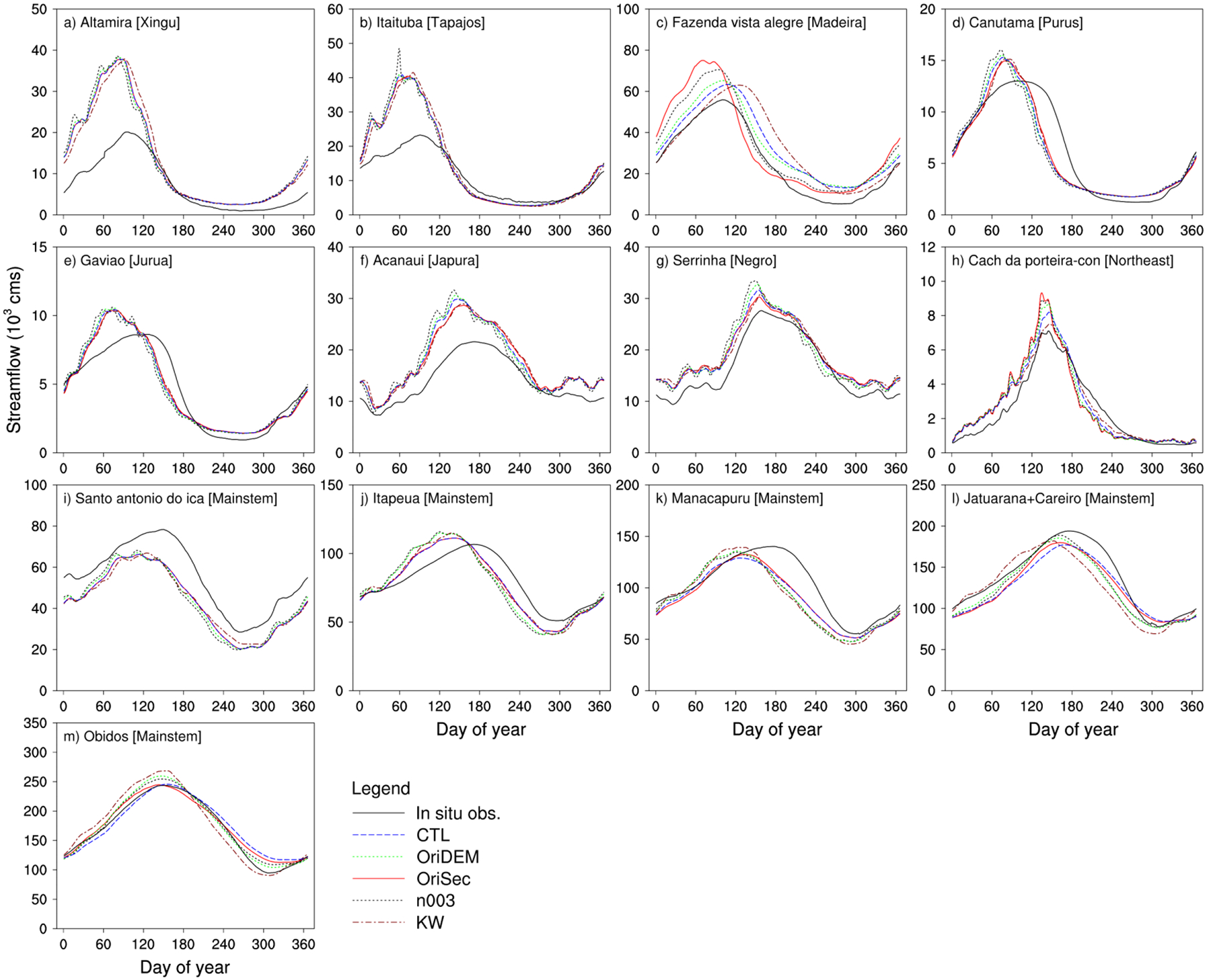
Observed and modeled average daily streamflow of 12 years (1995 – 2006) at 13 stream gauges. Setup of the five simulations is described in Table 2: CTL – Control simulation; OriDEM – Using the original DEM (with vegetation-caused biases); OriSec – Using basin-wide channel geometry formulae; n003 – Using a uniform Manning roughness coefficient (i.e., 0.03) for all the channels; KW – Using kinematic wave method to represent river flow.

Figure 12.

Differences in subbasin flooded fractions averaged during 13 years (1995 – 2007) between the control simulation (CTL) and the four contrasting simulations (i.e., OriDEM, OriSec, n003 and KW) for the high-water season (AMJ – April, May and June) and low-water season (OND – October, November and December): (a) and (b): CTL minus OriDEM; (d) and (e): CTL minus OriSec; (g) and (h): CTL minus n003; (j) and (k): CTL minus KW. Panel (c) shows DEM differences (CTL minus OriDEM); Panel (f) shows categories of cross-section changes for the 10 subregions; Panel (i) shows Manning coefficient differences (CTL minus n003).

Figure 8 shows the average seasonal cycles of observed and simulated streamflow during a period of 12 years (1995 – 2006) at 13 stream gauges. Figure 9 shows the observed and modeled river stages at daily scale in year 2007 for 11 subbasins containing or close to 11 of the 13 gauges. Figure 10 illustrates the simulated average river surface profiles along the mainstem in the four seasons (i.e., rising flood, high water, falling flood and low water) of year 2007. Figure 11 demonstrates the average seasonal cycles of observed and simulated flood extent during 13 years (1995 – 2007) for the 10 subregions and the entire basin. In Figs. 8 – 11, the results of all five simulations are included. Figure 12 reveals the differences in average inundation spatial patterns of 13 years (1995 – 2007) between the control simulation and the four contrasting simulations for the high-water and low-water seasons, respectively. In the following discussions, Figs. 8 – 12 are used jointly to reveal the impacts of the four factors on surface water dynamics.

Figure 9.

Observed and modeled river stages at the daily scale in year 2007 for the subbasins containing or close to 11 of the 13 stream gauges. Setup of the five simulations is described in Table 2: CTL – Control simulation; OriDEM – Using the original DEM (with vegetation-caused biases); OriSec – Using basin-wide channel geometry formulae; n003 – Using a uniform Manning roughness coefficient (i.e., 0.03) for all the channels; KW – Using kinematic wave method to represent river flow.

Figure 10.

Modeled average river surface profiles along the mainstem in the four seasons of year 2007: (a) JFM (January, February and March; the period of rising flood); (b) AMJ (April, May and June; the period of high water); (c) JAS (July, August and September; the period of falling flood); and (d) OND (October, November and December; the period of low water). Results of 5 simulations are shown.The curves in the right half panel (0 – 1500 km) use the right y-axis except the riverbed profile. The five stream-gauge locations are labeled on the x-axis: San – Santo Antonio do ica; Ita – Itapeua; Man – Manacapuru; J+C – Jatuarana+Careiro; Obi – Obidos. Riverbed slope (e) and Manning roughness coefficients (f) along the mainstem are also shown. In the panel (f), the solid curve shows spatially varied Manning coefficients used in four simulations; the dotted line shows the uniform Manning coefficient of 0.03 used in the simulation “n003”.

Figure 11.

Observed and modeled average monthly flood extent of 13 years (1995 – 2007) for the 10 subregions and the entire Amazon Basin. Setup of the five simulations is described in Table 2: CTL – Control simulation; OriDEM – Using the original DEM (with vegetation-caused biases); OriSec – Using basin-wide channel geometry formulae; n003 – Using a uniform Manning roughness coefficient (i.e., 0.03) for all the channels; KW – Using kinematic wave method to represent river flow.

4.1. Correction of DEM

The vegetation-caused biases in the HydroSHEDS DEM data were alleviated via DEM correction. This lowered the floodplain elevations and changed the slope of the elevation profile, which could lead to changes in simulated flood extent. Figure 11 shows that the DEM correction increases flood extent in all 10 subregions. The increase of inundation postpones and lowers streamflow peaks in the downstream channels, especially in the middle and lower mainstem (Figs. 8 j – m).

The increase of inundation also brings about changes in river stages: the magnitude of river stage fluctuations is reduced in the 11 subbasins (Fig. 9). In the middle mainstem, the river stages averaged over three months is lowered in the rising-flood and high-water seasons (Figs. 10a and 10b) and elevated in the falling-flood and low-water seasons (Figs. 10c and 10d), with magnitude up to about 1 m.

Figures 12a and 12b show that DEM correction leads to inundation changes in many subbasins: while flood extent is mostly enlarged, DEM correction could increase the slope of the elevation profile in some subbasins and reduce flood extent.

4.2. Adjustment of channel geometry

Adjusting channel cross-sectional geometry could affect the simulated surface water area from two aspects: (1) reducing channel cross-sectional area, which is equivalent to reducing channel storage capacity, could increase flooded area over floodplains, and vice versa; (2) broadening the channel width, hence increasing channel surface area, and vice versa. The nine tributary subregions can be placed in five categories according to the changes of channel cross-sectional area, the channel width and the total surface water area (Table 3). The channel geometry of the mainstem is not adjusted. The inundation changes in the tributary subregions affect streamflow in the mainstem and slightly delays and attenuates the inundation peak there (Fig. 11j).

Table 3.

Adjusting channel cross-sectional geometry affects inundated area in tributary subregions.^a

Category	Cross-sectional areab	Inundated area over floodplains	Channel widthc	Channel area	Total surface water aread	Subregions
A	−	+	+	+	+	h) Negro
B	−	+	−	−	+	c) Madeira; i) Northeast
C	+	−	+	+	+	b) Tapajos; g) Japura
D	+	−	−	−	−	d) Purus; e) Jurua
E	No adjusting	No change	No adjusting	No change	No change	a) Xingu; f) Upper-Solimoes tributaries

Note:

^a.‘+’ means increase; ‘−’ means decrease;

^b.This variation depends on the factor α_A in Table 1: α_A >1: ‘+’; α_A <1: ‘−’; α_A =1: ‘No adjusting’;

^c.This variation depends on the factor α_w in Table 1: α_w >1: ‘+’; α_w <1: ‘−’; α_w =1: ‘No adjusting’;

^d.This change is shown by inundation results in Fig. 11.

Figure 8c shows that channel geometry changes significantly postpone and lower the streamflow peak at the gauge in the lower Madeira subregion. The reason is that channel geometry changes evidently advance inundation in this subregion (Fig. 11c). Inundation changes in other subregions are comparatively smaller than that of the Madeira subregion and do not result in significant alterations in streamflow (Fig. 8).

Adjustment of channel geometry could have evident effect on the river stage of the local channel. The mechanism for channel geometry changes to affect river stages is not straightforward. For instance, reducing the channel width could raise the river stage and hence increase the flow velocity or inundation, which, in turn tend to lower the river stage (Fig. 13). The simulated results of this study show that, in most circumstances, reducing the channel width raises the river stage of the local channel (Figs. 9b, 9c and 9d) and vice versa (Figs. 9e and 9f). In Fig. 9a, this rule does not apply from about day 170 to 330, which could be caused by backwater effects: the river stage of this channel is influenced by that of the mainstem section downstream of the Obidos gauge.

Figure 13.

An example of the effects of channel cross-sectional geometry on the water depth of the local channel.

Channel geometry changes could also influence river stages of remote downstream channels. The channel morphology of the mainstem is not adjusted. So the river stage changes along the mainstem are caused by inundation changes in the upstream area. The channel-geometry adjustment of this study advances inundation in the major portion of the Amazon Basin, which influences river stages along the mainstem, particularly in the middle reaches: the river stages averaged over three months are lowered in the rising-flood and high-water seasons (Figs. 10a and 10b) and elevated in the falling-flood and low-water seasons (Figs. 10c and 10d), with magnitude up to about 1 m. The phenomenon can also be observed in Figs. 9h–k.

4.3. Varying the Manning coefficients

The streamflow Nash–Sutcliffe efficiency coefficients (NSEs) of the simulation ‘CTL’ were compared with those of the simulation ‘n003’ (Table 4). It is shown that the NSEs of the simulation ‘CTL’ are evidently higher than those of the simulation ‘n003’ at 12 of the 13 gauges (the NSE decreases slightly from 0.931 to 0.911 at the Obidos gauge), which suggests that the spatially varied Manning coefficients are more appropriate than the uniform Manning coefficient (i.e., 0.03) for the simulations of this study.

Table 4.

Nash–Sutcliffe efficiency coefficients (NSEs) of modeled daily streamflow of 12 years (1995 – 2006) at the 13 stream gauges for the simulations ‘CTL’ and ‘n003’.

Gauge index	Gauge name	NSE of Simulation ‘CTL’	NSE of Simulation ‘n003’	Subregion of the gauge
a	Altamira	− 0.677	− 0.889	Xingu
b	Itaituba	− 0.310	− 0.420	Tapajos
c	Fazenda vista alegre	0.782	0.701	Madeira
d	Canutama	0.678	0.567	Purus
e	Gaviao	0.512	0.389	Jurua
f	Acanaui	− 0.160	− 0.604	Japura
g	Serrinha	0.748	0.546	Negro
h	Cach da porteira-con	0.767	0.674	Northeast
i	Santo antonio do ica	0.428	0.297	Mainstem
j	Itapeua	0.570	0.140	Mainstem
k	Manacapuru	0.623	0.407	Mainstem
l	Jatuarana+Careiro	0.819	0.787	Mainstem
m	Obidos	0.911	0.931	Mainstem

The spatially varied Manning coefficients resulted in larger flood extent than the uniform coefficient of 0.03 (Fig. 11). The spatially varied coefficients range from 0.03 to 0.05 and are equal to or larger than the uniform coefficient. The larger Manning coefficient leads to the lower flow velocity, larger wet cross-sectional area and thereby higher river stage (Fig. 9), which advance local inundation, as well as upstream inundation due to backwater effects. Inundation increases in the upstream area postpone and attenuate flood waves at the downstream gauges (Fig. 8).

Increases of the Manning coefficients not only affect local and upstream river stages as discussed above, but also influence downstream river stages. Inundation increases in the upstream area have impact on streamflow rates and hence river stages in the downstream channels. Therefore river stages are influenced by not only downstream and local Manning coefficients, but also upstream Manning coefficients. Figure 9 shows that the varied Manning coefficients result in rise of river stages in most circumstances, which suggests that the local and downstream effects play a dominant role: increases of Manning coefficients reduce flow velocities, enlarge wet cross-sectional area and hence elevate river stages. However, in the lower mainstem the upstream effects may overwhelm the local and downstream effects. For instance, Fig. 9k shows that, during the rising-flood period (before about the day 150), the varied Manning coefficients reduce river stages at the Obidos gauge. The main reason is that the varied Manning coefficients increase inundation in the upstream area, which results in smaller streamflow rates in the lower mainstem for the rising-flood period.

4.4. Backwater effects

Besides the above factors, backwater effects also play a significant role in the surface water dynamics of the Amazon Basin, particularly in the middle and lower portions of this basin which have very mild topography (e.g., Fig. 10e). In this study, backwater effects were represented by using the diffusion wave method to simulate water flow through channels in four of the five simulations (including the control simulation). In the remaining simulation (i.e., KW), the diffusion wave method was replaced with the kinematic wave method which could not represent backwater effects. The results of the control simulation were compared with those of the simulation KW to reveal backwater effects on surface water dynamics.

In the diffusion wave method, backwater effects could decrease the friction slope and hence reduce the flow velocity (Eqs. (1) and (2)), and vice versa. For the same streamflow rate, reduction of the flow velocity leads to larger wet cross-sectional area and thereby higher river stage, which could increase local inundation if the river stage exceeds the bank top, as well as increase upstream inundation due to backwater effects. This mechanism is similar to the aforementioned mechanism that increases of the Manning roughness coefficients could advance local and upstream inundation. Using the same reasoning, backwater effects also could increase the flow velocity and eventually reduce inundation. Figure 11 shows that the flood extent of the control simulation is larger than that of the simulation KW for nine of the ten subregions and the entire Amazon Basin, which suggests that the dominant role of backwater effects is to advance inundation for this basin. However, backwater effects also could reduce inundation as demonstrated in the subregion “Upper-Solimoes tributaries” (Fig. 11f). Figures 12j and 12k illustrate that backwater effects tend to advance inundation in the middle and lower mainstem, lower Negro and lower Madeira subregions, where the topography is flat and the streamflow rate is comparatively high.

Backwater effects bring about inundation increases in the subbasins of the upstream area, which have impact on streamflow in the downstream channels. Inundation increases in the upstream area could delay and attenuate hydrographs in the middle and lower mainstem (Figs. 8k–m). These backwater effects on hydrographs agree with the results of Paiva et al. (2013).

Backwater effects could increase the friction slope and hence advance the flow velocity, which resulted in changes of the hydrograph. For instance, Fig. 8c shows that at the lower Madeira River the flow peak of the control simulation is about 20 days earlier than that of the simulation ‘KW’. The Madeira River reaches its highest stage about 1 – 2 months earlier than the mainstem (compare Fig. 9b and Fig. 9j; also see Meade et al., 1991). This time difference in peak stage makes the slope of the river surface steep in the rising-flood period of the Madeira River, which advances the flow velocity and brings the streamflow peak to an earlier time. This phenomenon of backwater effects on the streamflow timing cannot be captured in the simulation ‘KW’ because in the kinematic wave method the flow velocity depends on the riverbed slope instead of the river surface slope.

It is discussed above that backwater effects could influence local and upstream river stages by changing the local flow velocity, but they could also affect downstream flow rates, which consequently influence downstream river stages. Therefore the river stage of a channel is influenced by not only the local and downstream backwater effects, but also the backwater effects in the upstream area. The combined impact significantly attenuates both temporal (Fig. 9) and spatial (Fig. 10) river stage fluctuations. This result is consistent with that of Yamazaki et al. (2011), which primarily discussed the river stages at the Obidos gauge and the river surface profiles of the mainstem in one month, while this study examined river stages of 11 major gauges on tributaries or the mainstem (Fig. 9), and the river surface profiles of the mainstem in four seasons (Fig. 10).

Figure 10 also shows that the river stages of the middle and lower mainstem drop significantly when backwater effects are not represented, especially during the rising-flood, falling-flood and low-water periods (Figs. 10a, 10c and 10d). The sea level was used as the boundary condition at the basin outlet when the diffusion wave method was employed to simulate water flow in channels. The river stages of the middle and lower mainstem were influenced by the sea level via backwater effects. In this study the sea level was assumed to be fixed. In reality, the sea level rises and falls regularly, which exerts varying impact on river flow (e.g., Yamazaki et al., 2012). The effect of sea level variation on river hydrology could be represented after the surface-water transport model is coupled with an Earth system model. Furthermore, this modeling framework could be used to investigate the potential impact of sea level rise on the terrestrial hydrologic cycle due to climate change.

5. Discussion and conclusion

Continental-scale modeling of surface hydrology in the Amazon Basin faced a few challenges including uncertainties in parameters of floodplain and channel morphology, and representation of river flow over flat-gradient topography. This study aimed to tackle those uncertainties and improve the continental-scale modeling of surface water dynamics in this vast basin. A macro-scale inundation scheme was integrated with the MOSART surface-water transport model and the extended model was utilized. Vegetation-caused biases embedded in the HydroSHEDS DEM data were alleviated by using a vegetation height map at about 1-km resolution (Simard et al., 2011) and a land cover dataset at about 90-m resolution for wetlands of the lowland Amazon Basin (Hess et al., 2003, 2015). Channel cross-sectional geometry was estimated by using relationships between channel cross-sectional dimensions and upstream drainage area (referred to as channel geometry formulae). The general channel geometry formulae for the entire basin (Beighley and Gummadi, 2011) were adjusted for most subregions based on channel morphological information of local locations. The Manning roughness coefficient for the channel depended on the channel depth to reflect the general rule that the relative importance of riverbed resistance in river flow declined with the increase of river size.

The simulated results were evaluated against in situ streamflow data as well as remote sensing river-stage and inundation data. The simulated streamflow results were compared with the observed data from 13 major stream gauges. The hydrographs were reproduced fairly well for the majority of the 13 gauges. For the 11 subbasins containing or close to 11 of the 13 gauges, the simulated river stages were compared to the altimetry data obtained by the Envisat satellite. The timing (magnitude) of river stage fluctuations was captured well for all (the majority) of the 11 subbasins. For the 10 subregions and the entire basin, the simulated inundation results were compared against the GIEMS satellite data (Papa et al., 2010; Prigent et al., 2007, 2012). The simulated inundation results were comparable to the GIEMS observations for the major portion of the basin. The flood extent discrepancies between the simulation and observations could be partially explained by biases of runoff inputs. Those discrepancies could also be due to uncertainties in geomorphological parameters, missing representations of some potentially important hydrologic processes, as well as biases of the GIEMS data.

Sensitivity analyses were conducted to investigate the impacts on surface water dynamics of the Amazon Basin by improving floodplain topography, channel morphology and Manning coefficients, as well as accounting for backwater effects. The results showed that all four factors could have evident effect on inundation, although through different mechanisms: DEM correction changes the floodplain elevations and slope; adjusting channel cross-sectional geometry changes the channel storage capacity; Manning coefficient variations or backwater effects affect the flow velocity and hence the river stage. Inundation changes in the upstream area affected the downstream surface water dynamics, particularly along the middle and lower mainstem Amazon, by delaying flood waves, as well as attenuating fluctuations of streamflow and river stages, which consequently brought about inundation changes in the downstream area. Channel cross-sectional geometry, the Manning coefficient and backwater effects had impacts on the river stage of the local channel, and potential influence on surface water dynamics of the upstream area due to backwater effects.

The understanding obtained in this study could be helpful to improving the modeling of terrestrial surface water dynamics at the global scale. Besides the Amazon Basin, alleviating the vegetation-caused biases in the DEM data is also worthwhile for other basins with considerable inundation and extensive forested area, such as the Congo Basin. The simple method we developed can be tested globally for its impacts on inundation modeling. It is shown that a simple method can improve the representation of channel cross-sectional geometry and consequently the modeled surface hydrology, which implies that representing the spatial diversity of channel morphology should be emphasized in applications for other regions. The future Surface Water and Ocean Topography (SWOT) mission (Alsdorf et al., 2007) is expected to bring notable advancement in this aspect. It is also demonstrated that spatially varied Manning roughness coefficients depending on the channel depth result in streamflow hydrographs better than those of the uniform Manning coefficient. It is worth investigating the application of this method to other regions, although the Manning coefficient is empirical and model dependent. Besides the Amazon River, it is very likely that backwater effects also play a significant role in many other rivers, such as the Yangtze River and Mississippi River (Meade et al., 1991). Therefore backwater effects should be accounted for in the global applications where river stages, inundation extent or river flow velocities are investigated. These methods may have impacts on surface hydrology to different degrees for various regions. For instance, DEM correction and backwater effects are expected to have larger impacts on surface hydrology in regions with milder topography.

Subbasins are used as computation units in this study. Surface hydrologic simulations using subbasins as computation units are less scale-dependent than those using square grids as computation units (e.g., Getirana et al., 2010; Tesfa et al., 2014a, 2014b). For instance, when computation units become coarser, using subbasin units can preserve pathways of river flows better than using grid units (e.g., Getirana et al., 2010). In this study, the simulated hydrologic results are comparable to observations, although the subbasin units are relatively coarse (with an average area of 1091.7 km²). For continental- or global- scale applications, using subbasin units could represent surface water transport more realistically than using grid units when the subbasin size is comparable to the grid size.

At the same time, some aspects of the model could be improved, such as the representation of water exchange between channels and floodplains. In this study, instantaneous channel–floodplain exchange is assumed, which could overestimate flooded area during the rising-flood period, and vice versa during the receding-flood period. The modeling of this exchange process could be improved by including a mechanistic representation of water flow over floodplains. For instance, Alsdorf et al. (2005) demonstrated that the floodplain drainage could be simulated using a linear diffusion model; Miguez-Macho and Fan (2012) used diffusion wave method to simulate two dimensional flow over floodplains. Moreover, the mechanistic representation of floodplain flow could be used to simulate water exchange over floodplains between neighboring subbasins which was not accounted for in this study.

In addition, the modeling of surface water dynamics could benefit from integrating the surface-water transport model with land surface models or climate models by representing the interactions between surface hydrology and subsurface water fluxes as well as atmospheric processes. Such interactions could potentially have important effects on surface fluxes, with important implications to modeling of land-atmosphere interactions and tropical forest response to floods and droughts.

References

- Alsdorf D, Dunne T, Melack J, Smith L and Hess L: Diffusion modeling of recessional flow on central Amazonian floodplains, Geophys. Res. Lett, 32(21), L21405, doi: 10.1029/2005GL024412, 2005. [DOI] [Google Scholar]
- Alsdorf DE, Rodríguez E and Lettenmaier DP: Measuring surface water from space, Rev. Geophys, 45(2), RG2002, doi: 10.1029/2006RG000197, 2007. [DOI] [Google Scholar]
- Arcement GJ and Schneider VR: Guide for selecting Manning’s roughness coefficients for natural channels and flood plains, United States Geological Survey, 1989. [Google Scholar]
- Baugh CA, Bates PD, Schumann G and Trigg MA: SRTM vegetation removal and hydrodynamic modeling accuracy, Water Resour. Res, 49(9), 5276–5289, doi: 10.1002/wrcr.20412, 2013. [DOI] [Google Scholar]
- Beighley RE and Gummadi V: Developing channel and floodplain dimensions with limited data: a case study in the Amazon Basin, Earth Surf. Process. Landf, 36(8), 1059–1071, doi: 10.1002/esp.2132, 2011. [DOI] [Google Scholar]
- Beighley RE, Eggert KG, Dunne T, He Y, Gummadi V and Verdin KL: Simulating hydrologic and hydraulic processes throughout the Amazon River Basin, Hydrol. Process, 23(8), 1221–1235, doi: 10.1002/hyp.7252, 2009. [DOI] [Google Scholar]
- Bousquet P, Ciais P, Miller JB, Dlugokencky EJ, Hauglustaine DA, Prigent C, Van der Werf GR, Peylin P, Brunke E-G, Carouge C, Langenfelds RL, Lathière J, Papa F, Ramonet M, Schmidt M, Steele LP, Tyler SC and White J: Contribution of anthropogenic and natural sources to atmospheric methane variability, Nature, 443(7110), 439–443, doi: 10.1038/nature05132, 2006. [DOI] [PubMed] [Google Scholar]
- Chow VT, Maidment DR and Mays LW: Applied Hydrology, McGraw-Hill, 1988. [Google Scholar]
- Coe MT, Costa MH and Howard EA: Simulating the surface waters of the Amazon River basin: impacts of new river geomorphic and flow parameterizations, Hydrol. Process, 22(14), 2542–2553, doi: 10.1002/hyp.6850, 2008. [DOI] [Google Scholar]
- Dai A and Trenberth KE: Estimates of Freshwater Discharge from Continents: Latitudinal and Seasonal Variations, J. Hydrometeorol, 3(6), 660–687, doi:, 2002. [DOI] [Google Scholar]
- Decharme B, Douville H, Prigent C, Papa F and Aires F: A new river flooding scheme for global climate applications: Off-line evaluation over South America, J. Geophys. Res. Atmospheres, 113(D11), D11110, doi: 10.1029/2007JD009376, 2008. [DOI] [Google Scholar]
- Decharme B, Alkama R, Douville H, Becker M and Cazenave A: Global Evaluation of the ISBA-TRIP Continental Hydrological System. Part II: Uncertainties in River Routing Simulation Related to Flow Velocity and Groundwater Storage, J. Hydrometeorol, 11(3), 601–617, doi: 10.1175/2010JHM1212.1, 2010. [DOI] [Google Scholar]
- Getirana ACV, Bonnet M-P, Rotunno Filho OC, Collischonn W, Guyot J-L, Seyler F and Mansur WJ: Hydrological modelling and water balance of the Negro River basin: evaluation based on in situ and spatial altimetry data, Hydrol. Process, 24(22), 3219–3236, doi: 10.1002/hyp.7747, 2010. [DOI] [Google Scholar]
- Getirana ACV, Boone A, Yamazaki D, Decharme B, Papa F and Mognard N: The Hydrological Modeling and Analysis Platform (HyMAP): Evaluation in the Amazon Basin, J. Hydrometeorol, 13(6), 1641–1665, doi: 10.1175/JHM-D-12-021.1, 2012. [DOI] [Google Scholar]
- Getirana ACV, Boone A, Yamazaki D and Mognard N: Automatic parameterization of a flow routing scheme driven by radar altimetry data: Evaluation in the Amazon basin, Water Resour. Res, 49(1), 614–629, doi: 10.1002/wrcr.20077, 2013. [DOI] [Google Scholar]
- Getirana ACV, Dutra E, Guimberteau M, Kam J, Li H-Y, Decharme B, Zhang Z, Ducharne A, Boone A, Balsamo G, Rodell M, Toure AM, Xue Y, Peters-Lidard CD, Kumar SV, Arsenault K, Drapeau G, Ruby Leung L, Ronchail J and Sheffield J: Water Balance in the Amazon Basin from a Land Surface Model Ensemble, J. Hydrometeorol, 15(6), 2586–2614, doi: 10.1175/JHM-D-14-0068.1, 2014. [DOI] [Google Scholar]
- Guimberteau M, Drapeau G, Ronchail J, Sultan B, Polcher J, Martinez J-M, Prigent C, Guyot J-L, Cochonneau G, Espinoza JC, Filizola N, Fraizy P, Lavado W, De Oliveira E, Pombosa R, Noriega L and Vauchel P: Discharge simulation in the sub-basins of the Amazon using ORCHIDEE forced by new datasets, Hydrol Earth Syst Sci, 16(3), 911–935, doi: 10.5194/hess-16-911-2012, 2012. [DOI] [Google Scholar]
- Hess LL, Melack JM, Novo EMLM, Barbosa CCF and Gastil M: Dual-season mapping of wetland inundation and vegetation for the central Amazon basin, Remote Sens. Environ, 87(4), 404–428, doi: 10.1016/j.rse.2003.04.001, 2003. [DOI] [Google Scholar]
- Hess LL, Melack JM, Affonso AG, Barbosa C, Gastil-Buhl M and Novo EMLM: Wetlands of the Lowland Amazon Basin: Extent, Vegetative Cover, and Dual-season Inundated Area as Mapped with JERS-1 Synthetic Aperture Radar, Wetlands, 35(4), 745–756, doi: 10.1007/s13157-015-0666-y, 2015. [DOI] [Google Scholar]
- Junk WJ, Piedade MTF, Wittmann F, Schöngart J and Parolin P, Eds.: Amazonian Floodplain Forests, Springer Netherlands, Dordrecht: [online] Available from: http://link.springer.com/10.1007/978-90-481-8725-6 (Accessed 25 March 2016), 2011. [Google Scholar]
- Li H, Wigmosta MS, Wu H, Huang M, Ke Y, Coleman AM and Leung LR: A Physically Based Runoff Routing Model for Land Surface and Earth System Models, J. Hydrometeorol, 14(3), 808–828, doi: 10.1175/JHM-D-12-015.1, 2013. [DOI] [Google Scholar]
- Meade RH, Rayol JM, Conceicão SCD and Natividade JRG: Backwater effects in the Amazon River basin of Brazil, Environ. Geol. Water Sci, 18(2), 105–114, doi: 10.1007/BF01704664, 1991. [DOI] [Google Scholar]
- Miguez-Macho G and Fan Y: The role of groundwater in the Amazon water cycle: 1. Influence on seasonal streamflow, flooding and wetlands, J. Geophys. Res, 117(D15), doi: 10.1029/2012JD017539, 2012. [DOI] [Google Scholar]
- de Paiva RCD, Buarque DC, Collischonn W, Bonnet M-P, Frappart F, Calmant S and Bulhões Mendes CA: Large-scale hydrologic and hydrodynamic modeling of the Amazon River basin, Water Resour. Res, 49(3), 1226–1243, doi: 10.1002/wrcr.20067, 2013. [DOI] [Google Scholar]
- Papa F, Prigent C, Aires F, Jimenez C, Rossow WB and Matthews E: Interannual variability of surface water extent at the global scale, 1993–2004, J. Geophys. Res. Atmospheres, 115(D12), D12111, doi: 10.1029/2009JD012674, 2010. [DOI] [Google Scholar]
- Prigent C, Papa F, Aires F, Rossow WB and Matthews E: Global inundation dynamics inferred from multiple satellite observations, 1993–2000, J. Geophys. Res. Atmospheres, 112(D12), D12107, doi: 10.1029/2006JD007847, 2007. [DOI] [Google Scholar]
- Prigent C, Papa F, Aires F, Jimenez C, Rossow WB and Matthews E: Changes in land surface water dynamics since the 1990s and relation to population pressure, Geophys. Res. Lett, 39(8), L08403, doi: 10.1029/2012GL051276, 2012. [DOI] [Google Scholar]
- Richey JE, Melack JM, Aufdenkampe AK, Ballester VM and Hess LL: Outgassing from Amazonian rivers and wetlands as a large tropical source of atmospheric CO2, Nature, 416(6881), 617–620, doi: 10.1038/416617a, 2002. [DOI] [PubMed] [Google Scholar]
- Sanders BF: Evaluation of on-line DEMs for flood inundation modeling, Adv. Water Resour, 30(8), 1831–1843, doi: 10.1016/j.advwatres.2007.02.005, 2007. [DOI] [Google Scholar]
- Simard M, Pinto N, Fisher JB and Baccini A: Mapping forest canopy height globally with spaceborne lidar, J. Geophys. Res. Biogeosciences, 116(G4), G04021, doi: 10.1029/2011JG001708, 2011. [DOI] [Google Scholar]
- Tesfa TK, Li H-Y, Leung LR, Huang M, Ke Y, Sun Y and Liu Y: A subbasin-based framework to represent land surface processes in an Earth system model, Geosci Model Dev, 7(3), 947–963, doi: 10.5194/gmd-7-947-2014, 2014a. [DOI] [Google Scholar]
- Tesfa TK, Ruby Leung L, Huang M, Li H-Y, Voisin N and Wigmosta MS: Scalability of grid- and subbasin-based land surface modeling approaches for hydrologic simulations, J. Geophys. Res. Atmospheres, 119(6), 2013JD020493, doi: 10.1002/2013JD020493, 2014b. [DOI] [Google Scholar]
- Trigg MA, Wilson MD, Bates PD, Horritt MS, Alsdorf DE, Forsberg BR and Vega MC: Amazon flood wave hydraulics, J. Hydrol, 374(1–2), 92–105, doi: 10.1016/j.jhydrol.2009.06.004, 2009. [DOI] [Google Scholar]
- Vörösmarty CJ, Moore B, Grace AL, Gildea MP, Melillo JM, Peterson BJ, Rastetter EB and Steudler PA: Continental scale models of water balance and fluvial transport: An application to South America, Glob. Biogeochem. Cycles, 3(3), 241–265, doi: 10.1029/GB003i003p00241, 1989. [DOI] [Google Scholar]
- Wilson M, Bates P, Alsdorf D, Forsberg B, Horritt M, Melack J, Frappart F and Famiglietti J: Modeling large-scale inundation of Amazonian seasonally flooded wetlands, Geophys. Res. Lett, 34(15), L15404, doi: 10.1029/2007GL030156, 2007. [DOI] [Google Scholar]
- Yamazaki D, Kanae S, Kim H and Oki T: A physically based description of floodplain inundation dynamics in a global river routing model, Water Resour. Res, 47(4), W04501, doi: 10.1029/2010WR009726, 2011. [DOI] [Google Scholar]
- Yamazaki D, Lee H, Alsdorf DE, Dutra E, Kim H, Kanae S and Oki T: Analysis of the water level dynamics simulated by a global river model: A case study in the Amazon River, Water Resour. Res, 48(9), W09508, doi: 10.1029/2012WR011869, 2012. [DOI] [Google Scholar]