Mathematical modeling of COVID-19 spreading with asymptomatic infected and interacting peoples

Abstract

In this article we propose a modified compartmental model describing the transmission of COVID-19 in Morocco. It takes account on the asymptomatic people and the strategies involving hospital isolation of the confirmed infected person, quarantine of people contacting them, and home containment of all population to restrict mobility. We establish a relationship between the containment control coefficient $c_0$ and the basic reproduction number ${\mathcal{R}}_0$. Different scenarios are tested with different values of $c_0$, for which the stability of a Disease Free Equilibrium point is correlated with the condition linking ${\mathcal{R}}_0$ and $c_0$. A worst scenario in which the containment is not respected in the same way during the period of confinement leads to several rebound in the evolution of the pandemic. It is shown that home containment, if it is strictly respected, played a crucial role in controlling the disease spreading.

Introduction

The infectious diseases was always a challenge of scientific to prevent the pandemic spreading. Virology, biology, medicine, epidemiology as well as mathematical modeling are involved in the understanding and fights against the spreading of virus. Mathematicians have addressed this problem several years ago, giving birth to a new pattern of the epidemiology, the so-called “mathematical epidemiology”, [1, 8, 9, 13, 25]. Compartmental models was built, with several configurations, to describe the dynamic of the virus, [5, 9, 19, 21, 22, 25]. In 1927, the concept of threshold was highlighted by Kermack and Mc Kendrick who established the famous threshold theorem [13]. It was proved that a threshold, representing the number of new cases resulting by an infectious individual in a susceptible population, and quantified by the basic reproduction number ${\mathcal{R}}_0$, allows crucial information on spreading of the disease. Indeed, ${\mathcal{R}}_0$ aims to ensure the stability of an equilibrium, mainly, a Disease-Free Equilibrium (DFE), since if ${\mathcal{R}}_0<1$ then the DFE is stable whereas it will be unstable if ${\mathcal{R}}_0>1$, [3, 6, 7, 13, 18].

In this work we are interested by the new disease Covid-19. It is well known that this disease is caused by SARS-CoV-2 virus which is a member of Coronavirus family. Covid-19 causes respiratory infections that may escalate to severe effects. The main transmission routes of the SARS-CoV-2 virus are through coughing, sneezing, contacting infected people, or touching items or surfaces that are contaminated with fecal traces [2]. The severity of this virus lies in its spreading speed throughout the world to becomes an epidemic.

In absence of the vaccine, governments adopted different types of strategies to prevent worsening of the epidemic, as containment, quarantine,... Against to government that opt for no restriction of people moving and following the idea that virus when infecting population, this last becomes immune to it and then the pandemic decreases to be a standard influenza infection, the Moroccan government has taken several measures to prevent the propagation of the virus: the hospital isolation of the individual that are confirmed to be infected, the quarantine of interacting people and the strictest containment strategy was imposed across the country, to restrict the population mobility.

Our goal in this work is to build a modified compartmental epidemiological (SIR) model describing the transmission of the SARS-CoV-2 virus under the policies adopted in Morocco. In this model we incorporates the isolation of infected people, we take account on the people moving freely and are infected but don’t have symptoms and added the measure of the quarantine of the people interacting with an affected individual. The model is then described by a dynamical system enclosing a closed population with Susceptible (S), confirmed Infected (I), Asymptomatic (A), Quarantined (Q), Recovered (R) and Died (D), peoples respectively. In literature, Several papers analyze the evolution of Covid-19 disease using (SIR) models, [4, 10–12, 14, 15, 20, 24, 27], in which asymptomatic and quarantined peoples are considered. the aim of these works is the calculus of the basic reproduction number ${\mathcal{R}}_0$, the study of the local and global equilibria stability and to analyze the impact of several factors as seasonal succession [24], meteorological conditions, vaccination strategy, free medical care for the diagnostic COVID-19 patient, [11] and some local control strategies adopted for some cities [12]. In some cases, an attention is given to stochastic approach, [15].

Our approach is different, since the relationship between the compartments is different, we observe that the totality of confirmed infected individual comes from the asymptomatic infected and quarantined people not from susceptible as explained in the beginning of the following section. The second feature lies in the fact that the model does not admit a stable endemic equilibrium point, but several Disease-Free Equilibria (DFE), since a coexistence of a stable number of infected and uninfected people is not realistic due to the nature of Covid-19 virus spreading. Actually, as observed, after the containment breaking, the number of new contamination increases in several countries. Finally, our object is different, since we establish a relationship between the pertinence of the containment strategies and a containment control coefficient.

Based on those considerations we build the model, study the positivity, boundness and calculate the basic reproduction number ${\mathcal{R}}_0$ for a Disease-Free Equilibrium. We discuss the containment strategy and establish a relationship between ${\mathcal{R}}_0$ and the containment control coefficient $c_0$, describing the degree of containment. We simulate several scenarios by changing $c_0$ and analyze the peaks of different situations and diagram phases. We highlight in these simulations the required relation between the $c_0$ and ${\mathcal{R}}_0$ together with the stability of a (DFE). Finally, we investigate in the simulations a worst scenario in which the containment is not respected in the same way with time, which leads to different coefficient $c_0$. Using three values of $c_0$, corresponding to three phases in the Morocco containment, we produce simulations that are very close to real data of active infected in Morocco.

This paper is organized as follows, in the second section we describe the model compartments, study the positivity, compute the basic reproduction number ${\mathcal{R}}_0$. In Sect. 3, we introduce the containment and establish the relation between ${\mathcal{R}}_0$ and the containment control coefficient $c_0$. Section 4, is devoted to simulations and discussion. We termine by a conclusion and perspectives.

Mathematical model

Model without containment

Our model is a modified (SIR) model, it is conceptually different from literature [11, 12, 15, 24] since to build our model we formulates some assumptions governing the interaction between compartments: firstly, we assume that the totality of confirmed infected individual comes from the asymptomatic infected and quarantined people not from susceptible. In fact, a susceptible person can be contaminated by an asymptomatic infected individuals and then becomes themselves, in the first step, asymptomatic infected. Indeed, in one hand, the contaminated individuals are contagious when they are asymptomatic, otherwise, they are hospitalized and isolated and then can’t infect others. On the other hand, once infected, a susceptible person goes through a virus incubation period (3–14 days) [2], at this stage, this person has no symptoms.

Secondly, we assume that the time scale is short enough so that natural births and deaths are neglected. We suppose also that a recovered person will be immunized and can’t be infected again.

Finally, we suppose that the population is closed and divided on six compartments of individuals, that are, S(t) Susceptible, I(t) Infected, A(t) Asymptomatic infected, Q(t) Quarantined, Recovered R(t) and Dead D(t).

The evolution of susceptible people is given by the following equation

$$\begin{array}{c}\hfill \dot{S}(t)=-S\beta (A+\alpha I)+\xi Q,\end{array}$$

where $-\beta SA$ describes susceptible individual that interacts with asymptomatic infected individuals, acquires infection with transmission rate (contact rate) $\beta$ and becomes hence asymptomatic infected. $-\alpha \beta SI$ models the proportion of susceptible people who have contacted a confirmed infected individual and are putted in quarantine with rate $\alpha$. $\xi Q$ is the proportion of quarantined population that are negatively diagnosed with a release rate of quarantined compartment $\xi$.

The second equation describes infected individuals

$$\begin{array}{c}\hfill \dot{I}(t)=\theta Q+\delta A-(\mu +d_I)I.\end{array}$$

The term $\theta Q$ describes the proportion of quarantined people that are diagnosed positive, $\theta$ is the rate of becoming contaminated. $\delta A$ is the proportion of asymptomatic people that becoming symptomatic with a rate $\delta$, the term $\mu I$ represents the portion of recovered people and $d_I$ is the disease death rate.

The third equation describes the evolution of asymptomatic infected people,

$$\begin{array}{c}\hfill \dot{A}(t)=\beta SA-(\delta +\lambda )A,\end{array}$$

where $\lambda A$ represents the portion of asymptomatic individual that recovering by their own immune systems, $\lambda$ is the recovering rate.

The equation of quarantined individual is given as

$$\begin{array}{c}\hfill \dot{Q}(t)=\alpha \beta SI-(\xi +\theta )Q,\end{array}$$

all terms are already evoked.

Equations of recovered and died peoples are respectively

$$\begin{array}{c}\hfill \dot{R}(t)=\mu I+\lambda A,\end{array}$$

and

$$\begin{array}{c}\hfill \dot{D}(t)=d_{I}I.\end{array}$$

The schematic diagram of all compartments interconnection is given in the Fig. 1.

Fig. 1.

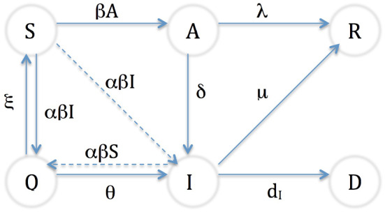
Diagram of the transition between compartments

All parameters involved in the model are positive constants.

Using the above depiction, the dynamical system modeling the spread of the SARS-CoV-2 virus is given as follows:

$$\begin{array}{c}\hfill \left\{\begin{array}{c}\dot{S}(t)=-\beta S(A+\alpha I)+\xi Q,\hfill \\ \dot{I}(t)=\theta Q+\delta A-(\mu +d_I)I,\hfill \\ \dot{A}(t)=\beta SA-(\delta +\lambda )A,\hfill \\ \dot{Q}(t)=\alpha \beta SI-(\xi +\theta )Q,\text{on}[0,t_f]\hfill \\ \dot{R}(t)=\mu I+\lambda A,\hfill \\ \dot{D}(t)=d_{I}I,\hfill \\ with\hfill \\ S(0)=S_0,I(0)=I_0,A(0)=A_0,Q(0)=Q_0,R(0)=R_0,D(0)=D_0.\hfill \end{array}\right)\end{array}$$ 1

The total accumulative population $N:=S(t)+I(t)+A(t)+Q(t)+R(t)+D(t)$ is constant since

$$\begin{array}{c}\hfill {\displaystyle \frac{\mathit{dN}}{\mathit{dt}}}=0.\end{array}$$

First of all, it is natural to ask whether this dynamical system provides a non-negative trajectories or not.

Proposition 1

All trajectories of the the system (1) starting in ${\mathbb{R}}_{+}^6$ are non-negative.

Proof

Remark firstly that from the equation of asymptomatic infected population in system (1), we get

$$\begin{array}{c}\hfill \dot{A}(t)=(\beta S-\delta -\lambda )A,\end{array}$$

which implies that

$$\begin{array}{c}\hfill A(t)=A(0)e^{{\displaystyle {\int }_0^t(\beta S(\tau )-\delta -\lambda )d\tau }}.\end{array}$$

Hence, for $A(0)\ge 0$, we obtain that

$$\begin{array}{c}\hfill A(t)\ge 0,\forall t\ge 0.\end{array}$$

Now we check the sign of vector field in the boundaries of ${\mathbb{R}}_{+}^6$. For $I=0$ and $Q\ge 0$ we have

$$\begin{array}{c}\hfill \dot{I}(t)=\theta Q+\delta A\ge 0,\end{array}$$

so, the vector field of I is pointed inside ${\mathbb{R}}_{+}^6$.

Similarly, for $Q=0$ and $S,I\ge 0$ we obtain

$$\begin{array}{c}\hfill \dot{Q}(t)=\alpha \beta SI\ge 0,\end{array}$$

and hence the vector field of Q is pointed inside ${\mathbb{R}}_{+}^6$. Using the same argument we prove that vector fields of S, R and D are pointed inside ${\mathbb{R}}_{+}^6$. We conclude then that all trajectories starting in ${\mathbb{R}}_{+}^6$ remains in it thereafter. $\square$

Proposition 2

All trajectories of the system (1) starting in ${\mathbb{R}}_{+}^6$ are bounded.

Proof

The positivity of the trajectories and the fact that ${\displaystyle \frac{\mathit{dN}}{\mathit{dt}}}(t)=0$, leads to boundedness of them. It follows that all trajectories starting in ${\mathbb{R}}_{+}^6$, belong to

$$\begin{array}{c}\hfill \{(S,I,A,Q,R,D)\in {\mathbb{R}}_{+}^6\mid S+I+A+Q+R+D=N\}.\end{array}$$

$\square$

Basic reproduction number ${\mathcal{R}}_0$

A practical and efficient tool to prevent the spread of an epidemic, is the basic reproduction number ${\mathcal{R}}_0$, it can be interpreted as “the number of secondary infections resulting from a single primary infection into an otherwise susceptible population”, see [3, 18]. Mathematically, we are interested by the value of ${\mathcal{R}}_0$ at an equilibrium corresponding to a constant susceptible population in absence of the infectious agent, commonly called the disease-free equilibrium (DFE). ${\mathcal{R}}_0$ aims to check the stability of DFE, if ${\mathcal{R}}_0>1$, then DFE is unstable and a sustainable spread of the pandemic occurs while if ${\mathcal{R}}_0<1$, DFE is asymptotically stable and the disease will die out.

We invoke the theory of next generation operator [3, 6, 18], to compute the basic reproduction number. Note that since the population is closed then we can compute D as

$$\begin{array}{c}\hfill D=N-S-I-Q-A-R,\end{array}$$

hence we restrict our self to infected, susceptible and recovered variables (A, I, Q, S, R), see [3, 18]. Consider now a DFE equilibrium $X^{\ast }=(S^{\ast },0,0,0,R^{\ast },D^{\ast })$ of the full system (1), with $S^{\ast }=N-R^{\ast }-D^{\ast }$ and $Y^{\ast }=(0,0,0,S^{\ast },R^{\ast })$ its restriction to subsystem (A, I, Q, S, R).

Following the same approach of [3], we consider the infected bloc $I_c=(A,I,Q)$,

$$\begin{array}{c}\hfill {\displaystyle \frac{d{I}_C}{\mathit{dt}}}(t)=\mathcal{H}(Y),\end{array}$$

where $Y=(A,I,Q,S,R)$ and

$$\begin{array}{c}\hfill \mathcal{H}(Y):=\left(\begin{array}{c}\beta SA-(\delta +\lambda )A\\ \theta Q+\delta A-(\mu +d_I)I\\ \alpha \beta SI-(\xi +\theta )Q\end{array}\right)\end{array}$$

Consider now, the Jacobian matrix $A=D_{I_C^{\ast }}\mathcal{H}$, where $I_C^{\ast }$ is such that $Y^{\ast }=(I_C^{\ast },S^{\ast },R^{\ast })=(0,0,0,S^{\ast },R^{\ast })$ is the DFE equilibrium.

We get

$$\begin{array}{c}\hfill A=\left(\begin{array}{ccc}-(\xi +\theta )& 0& \alpha \beta S^{\ast }\\ 0& \beta S^{\ast }-(\delta +\lambda )& 0\\ \theta & \delta & -(\mu +d_I)\end{array}\right).\end{array}$$

The matrix A can be decomposed on

$$\begin{array}{c}\hfill A=M-D,\end{array}$$

where

$$\begin{array}{c}\hfill M=\left(\begin{array}{ccc}0& 0& \alpha \beta S^{\ast }\\ 0& \beta S^{\ast }& 0\\ \theta & \delta & 0\end{array}\right)\text{and}D=\left(\begin{array}{ccc}(\xi +\theta )& 0& 0\\ 0& (\delta +\lambda )& 0\\ 0& 0& (\mu +d_I)\end{array}\right)\end{array}$$

We observe that $M\ge 0$ and $D>0$ is a diagonal matrix.

With those considerations, the basic reproduction number ${\mathcal{R}}_0$ is given by

$$\begin{array}{cc}\hfill {\overline{\mathcal{R}}}_0(S^{\ast })=& \rho (M{D}^{-1}),\hfill \\ \hfill =& max\left\{{\displaystyle \frac{\beta }{(\delta +\lambda )}},S^{\ast },,,\sqrt{{\displaystyle \frac{\alpha \beta \theta }{(\mu +d_I)(\xi +\theta )}}{S}^{\ast }}\right\}\hfill \end{array}$$ 2

where $\rho (B)$ denotes the spectral radius of the matrix B.

We obtain hence the following result which highlights the link between the stability of the DFE equilibrium $X^{\ast }=(S^{\ast },0,0,0,R^{\ast },D^{\ast })$ of the full system (1) and the threshold 1 of ${\overline{\mathcal{R}}}_0(S^{\ast })$.

Theorem 1

If ${\overline{\mathcal{R}}}_0(S^{\ast })>1$ then the DFE equilibrium $X^{\ast }$ is unstable.

If ${\overline{\mathcal{R}}}_0(S^{\ast })<1$, then the DFE equilibrium $X^{\ast }$ is asymptotically stable.

For the proof we can see [3].

Containment

As shown for the reproduction number, the eradication of the pandemic depends on the threshold value, 1, of ${\overline{\mathcal{R}}}_0(S^{\ast })$ at the disease-free equilibrium point, but this value depends on several parameters, among others $\beta$ and $S^{\ast }$. According to the expression of ${\overline{\mathcal{R}}}_0(S^{\ast })$ at a DFE equilibrium $X^{\ast }=(S^{\ast },0,0,0,R^{\ast },D^{\ast })$, the eradication of the pandemic is constrained by

$$\begin{array}{c}\hfill {\overline{\mathcal{R}}}_0(S^{\ast })<1,\end{array}$$

which is equivalent to fulfill

$$\begin{array}{c}\hfill {\displaystyle \frac{\beta }{(\delta +\lambda )}}{S}^{\ast }<1\end{array}$$

and

$$\begin{array}{c}\hfill \sqrt{{\displaystyle \frac{\alpha \beta \theta }{(\mu +d_I)(\xi +\theta )}}{S}^{\ast }}<1,\end{array}$$

which are equivalent to

$$\begin{array}{c}\hfill \beta <{\beta }_c(S^{\ast }):=min\left\{{\displaystyle \frac{\delta +\lambda }{S^{\ast }}},,,,{\displaystyle \frac{(\mu +d_I)(\xi +\theta )}{\alpha \theta S^{\ast }}}\right\}.\end{array}$$ 3

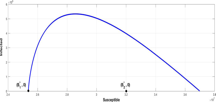
So, it’s necessary that the transmission rate $\beta$ of the virus must be lower than a critical level ${\beta }_c(S^{\ast })$ depending on $S^{\ast }$. Hence, with a high spreading virus ($\beta$ large), to be stable, a DFE must have ${\displaystyle \frac{\delta +\lambda }{S^{\ast }}}$ and ${\displaystyle \frac{(\mu +d_I)(\xi +\theta )}{\alpha \theta S^{\ast }}}$ sufficiently larges, which can occurs with small values of $S^{\ast }$ and in presence of suitable parameters values. This fact can be interpreted, since the population is closed, as there is a large number of infected individuals and the pandemic achieves a high peak before to decrease, as shown in Fig. 2.

Fig. 2.

The components $(S_1,I_1)=(S_1^{\ast },0)$ of a stable FDE point $X_1^{\ast }=(S_1^{\ast },0,A_1^{\ast },Q_1^{\ast },R_1^{\ast },D_1^{\ast })$ and the components $(S_2,I_2)=(S_2^{\ast },0)$ of an unstable FDE point $X_2^{\ast }=(S_2^{\ast },0,A_2^{\ast },Q_2^{\ast },R_2^{\ast },D_2^{\ast })$, with $S_1^{\ast }<S_2^{\ast }$

To avoid the outbreak of the pandemic, the transmission rate must be controlled, but it is well known that $\beta$ depends on whether the virus is spreading, which depends itself on the population managing strategy adopted by governments. Among control strategies used to prevent spreading of disease, the containment for all people throughout the country, is used to restrict the population mobility and limit the possibility of contamination. With this strategy we can reduce the spreading rate.

Let $c_0$ be the containment control coefficient with which we can reduce spreading of pandemic, the value of $c_0$ is correlated to whether the containment is made. We define hence a new rate of contamination (contact)

$$\begin{array}{c}\hfill {\beta }^{\prime }={\displaystyle \frac{1}{c_0}}\beta ,\end{array}$$ 4

and substitute in the model (1) the factor $\beta$ by ${\beta }^{\prime }$. We show now that a DFE equilibrium point $X^{\ast }=(S^{\ast },0,0,0,R^{\ast },D^{\ast })$, to be stable, must be such that the containment control coefficient $c_0$ is upper than the basic reproduction number ${\overline{\mathcal{R}}}_0$ for the model without containment.

Corollary 1

Consider the system (1) with containment control coefficient $c_0$. Then a DFE equilibrium point $X^{\ast }=(S^{\ast },0,0,0,R^{\ast },D^{\ast })$ is stable if

$$\begin{array}{c}\hfill c_0>{\overline{\mathcal{R}}}_0(S^{\ast }).\end{array}$$ 5

Proof

In the case where $\beta$ is substituted by ${\beta }^{\prime }$ of the Eq. (4), the basic reproduction number will be given by

$$\begin{array}{c}\hfill {\mathcal{R}}_0(c_0,S^{\ast })=max\left\{{\displaystyle \frac{\beta }{c_0(\delta +\lambda )}},S^{\ast },,,\sqrt{{\displaystyle \frac{\alpha \beta \theta }{c_0(\mu +d_I)(\xi +\theta )}}{S}^{\ast }}\right\}.\end{array}$$

As shown in theorem (1), to be stable, the DFE point $X^{\ast }$ must be such that

$$\begin{array}{c}\hfill {\mathcal{R}}_0(c_0,S^{\ast })<1,\end{array}$$

we get then

$$\begin{array}{c}\hfill c_0>max\left\{{\displaystyle \frac{\beta }{(\delta +\lambda )}},S^{\ast },,,\sqrt{{\displaystyle \frac{\alpha \beta \theta }{(\mu +d_I)(\xi +\theta )}}{S}^{\ast }}\right\}\end{array}$$

which means that

$$\begin{array}{c}\hfill c_0>{\overline{\mathcal{R}}}_0(S^{\ast }).\end{array}$$

$\square$

Let us remark that for $c_0=1$ there is no containment and in this case

$$\begin{array}{c}\hfill {\overline{\mathcal{R}}}_0(S^{\ast })={\mathcal{R}}_0(1,S^{\ast }).\end{array}$$

Numerical simulations

Our hope in this section is to illustrate with simulations the outcomes of previous sections. Let us first discuss the estimation of the parameters values based on literature and the publicly announced data by Moroccan government. The contamination rate

$$\begin{array}{c}\hfill \beta =s{\displaystyle \frac{p}{N}},\end{array}$$

where s is te number of contacts that a person can meet in one day, estimated at $s=40$ persons, and p is the percentage of contamination for an infected individual in one day, estimated at $p\approx 3\%$, see [17, 23]. $N=37·{10}^6$ is the Moroccan population. Hence

$$\begin{array}{c}\hfill \beta =0.324324·{10}^{-7}.\end{array}$$

The rate of quarantined individual that becoming infected, $\theta$ is estimated by using the average of confirmed infected individual proportions among quarantined peoples, see [16].

The Release rate from quarantined to susceptible people is given as

$$\begin{array}{c}\hfill \xi =1-\theta ,\end{array}$$

where

$$\begin{array}{c}\hfill \theta ={\displaystyle \frac{\text{Number}\text{of}\text{quarantined}\text{people}\text{becoming}\text{infected}}{\text{Number}\text{of}\text{quarantined}\text{people}}}.\end{array}$$

The value of $\theta$ is given in Table 1 with an interval range taking account of data in [16].

Table 1.

Model (1) parameters

Parameter	Description	Estimated value	Interval range	References
$\beta$	Contamination rate	$0.324324·{10}^{(-7)}$	–	[17, 23]
$\alpha$	Rate of quarantined susceptible peoples that contacting an infected individual	0.16	–	[11]
$\xi$	Release rate from quarantined to susceptible	0.872	$[0.86,0.9]$	$1-\theta$
$\theta$	Rate of quarantined becoming infected	0.128	$[0.14,0.1]$	[16]
$\delta$	Release rate from asymptomatic to symptomatic	0.2	–	$1-\lambda$
$\mu$	Rate of recovering from infected	0.15	–	[16]
$d_I$	Infecting died rate	0.039	–	[16]
$\lambda$	Rate of recovering from asymptomatic people	0.8	–	[26]

All values of parameters are listed in the Table 1.

We simulate the actual and forecast evolution of the epidemic in Morocco under different values of the control coefficient $c_0$ using Matlab software.

We suppose the evolution starts from $(S_0,I_0,A_0,Q_0,R_0,D_0)=(N-68,1,7,60,0,0)$ at 02 march 2020.

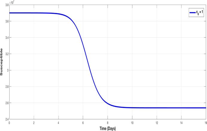
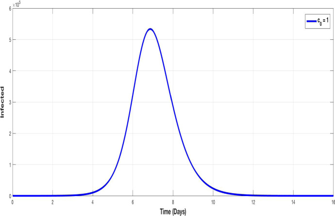
Figures 3 and 4 illustrate the evolution of susceptible and infected populations respectively, for $c_0=1$, i.e. without containment. We observe that the decline of susceptible population is accentuated and the infection achieves a very high peak.

Fig. 3.

The evolution of susceptible population without containment $c_0=1$

Fig. 4.

The evolution of infected population without containment $c_0=1$

For $S^{\ast }=N-{10}^6=S^{\ast }=3.6·{10}^7$, the pandemic is still spreading, and we have

$$\begin{array}{c}\hfill {\mathcal{R}}_0(1,S^{\ast })={\overline{\mathcal{R}}}_0(S^{\ast })=1.1676,\end{array}$$ 6

which bear out the condition (5), since

$$\begin{array}{c}\hfill c_0\ngtr {\overline{\mathcal{R}}}_0(S^{\ast }).\end{array}$$

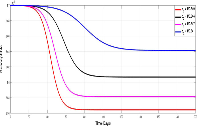
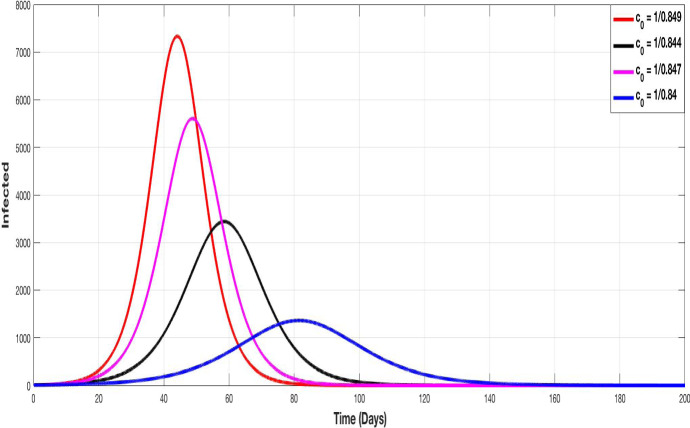
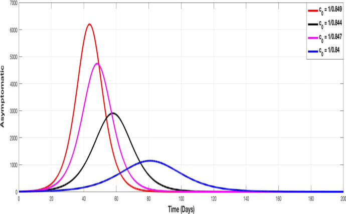
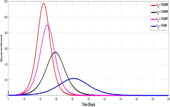
Figures 5, 6, 7 and 8 represent the evolution of S, I, A and Q curves, in which we test different values of containment control coefficient $c_0$ to show the impact of containment on the pandemic spreading. We choose $c_0={\displaystyle \frac{1}{0.849}}$, $c_0={\displaystyle \frac{1}{0.847}}$, $c_0={\displaystyle \frac{1}{0.844}}$ and $c_0={\displaystyle \frac{1}{0.84}}$ as degrees of containment respect. The choice of $c_0$ values remains theoretical but illustrative, we choose them closer together since a very small variation on it, provides a very important change in the evolution of curves.

Fig. 5.

The evolution of susceptible population with different values of the control containment coefficient $c_0$

Fig. 6.

The evolution of infected population with different values of the control containment coefficient $c_0$

Fig. 7.

The evolution of asymptomatic population with different values of the control containment coefficient $c_0$

Fig. 8.

The evolution of quarantined population with different values of the control containment coefficient $c_0$

Figure 5 shows that the higher is the containment control coefficient $c_0$ (i.e. containment more respected), the more susceptible population is conserved. Figure 6 illustrates the evolution of infected population. The higher is $c_0$, the lower is the peak.

The same conclusion can made for Figs. 7 and 8 since increasing $c_0$ has as consequence the decrease of peak of asymptomatic and quarantined population respectively.

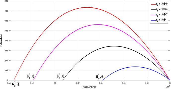
Figure 9 is an illustration of the phase diagram (S, I), it is observed that the higher is the coefficient $c_0$, the lower is the peak of infected people and the higher is the number of susceptible at the DFE equilibrium. Indeed, we have

$$\begin{array}{c}\hfill S_3^{\ast }\left(c_0,=,{\displaystyle \frac{1}{0.849}}\right)<S_4^{\ast }\left(c_0,=,{\displaystyle \frac{1}{0.847}}\right)<S_5^{\ast }\left(c_0,=,{\displaystyle \frac{1}{0.844}}\right)<S_6^{\ast }\left(c_0,=,{\displaystyle \frac{1}{0.84}}\right).\end{array}$$

Comparing this situation with that where there is no containment (6), i.e. where $c_0=1$, we get with the same value $S^{\ast }=3.6·{10}^7$ that

$$\begin{array}{cc}& {\mathcal{R}}_0(c_0,S^{\ast })=0.9913,\text{for}{c}_0={\displaystyle \frac{1}{0.849}},\hfill \\ \hfill & {\mathcal{R}}_0(c_0,S^{\ast })=0.9889,\text{for}{c}_0={\displaystyle \frac{1}{0.847}},\hfill \\ \hfill & {\mathcal{R}}_0(c_0,S^{\ast })=0.9854,\text{for}{c}_0={\displaystyle \frac{1}{0.844}}\hfill \end{array}$$

and

$$\begin{array}{c}\hfill {\mathcal{R}}_0(c_0,S^{\ast })=0.9808,\text{for}{c}_0={\displaystyle \frac{1}{0.84}},\end{array}$$

It is clear that with the containment the equilibrium point $X^{\ast }=(S^{\ast },0,0,0,R^{\ast },D^{\ast })$ is stable and the pandemic can be eradicated, this conclusion is perfectly in accordance with the condition (5), since the small value of $c_0$ is such that

$$\begin{array}{c}\hfill {\displaystyle \frac{1}{0.849}}=1.1778>{\overline{\mathcal{R}}}_0(S^{\ast })=1.1676.\end{array}$$

Consider now a DFE equilibrium with $S_6^{\ast }\approx 3.642·{10}^7$, calculate the basic reproduction number ${\mathcal{R}}_0(c_0,S_6^{\ast })$ for each $c_0$.

Fig. 9.

The phase diagram of (S, I) with DFE equilibria associated to different values of $c_0$

The calculus give

$$\begin{array}{c}\hfill {\mathcal{R}}_0(c_0,S_6^{\ast })=1.0028,\text{for}{c}_0={\displaystyle \frac{1}{0.849}}\end{array}$$

and

$$\begin{array}{c}\hfill {\mathcal{R}}_0(c_0,S_6^{\ast })=1.0005,\text{for}{c}_0={\displaystyle \frac{1}{0.847}}.\end{array}$$

It appear that for the control containment coefficient $c_0$ equal at ${\displaystyle \frac{1}{0.849}}$ or ${\displaystyle \frac{1}{0.847}}$ the equilibrium point is unstable, since ${\mathcal{R}}_0(c_0,S_6^{\ast })>1$, which can be interpreted by the fact that the condition (5) is violated:

$$\begin{array}{c}\hfill {\displaystyle \frac{1}{0.849}}=1.1778<{\overline{\mathcal{R}}}_0(S_6^{\ast })=1.1812\end{array}$$

and

$$\begin{array}{c}\hfill {\displaystyle \frac{1}{0.847}}=1.1806<{\overline{\mathcal{R}}}_0(S_6^{\ast })=1.1812,\end{array}$$

On the other hand, we have

$$\begin{array}{c}\hfill {\mathcal{R}}_0(c_0,S_6^{\ast })=0.9969,\text{for}{c}_0={\displaystyle \frac{1}{0.844}}\end{array}$$

and

$$\begin{array}{c}\hfill {\mathcal{R}}_0(c_0,S_6^{\ast })=0.9922,\text{for}{c}_0={\displaystyle \frac{1}{0.84}}.\end{array}$$

The equilibrium point with component $S_6^{\ast }$ is stable which comes from the fact that the condition (5) is fulfilled, indeed:

$$\begin{array}{c}\hfill {\displaystyle \frac{1}{0.844}}=1.1848>{\overline{\mathcal{R}}}_0(S_6^{\ast })=1.1812\end{array}$$

and

$$\begin{array}{c}\hfill {\displaystyle \frac{1}{0.84}}=1.1904>{\overline{\mathcal{R}}}_0(S_6^{\ast })=1.1812.\end{array}$$

The simulations of the containment strategy throughout the control containment coefficient $c_0$ show the efficiency of this strategy to reduce the magnitude of the epidemic and prevent spreading of it.

Worst scenario

In this subsection of simulation we would test a worst case in which the home containment is not respected in the same way throughout all duration of the containment. This fact can be interpreted by the changing in the containment control coefficient. As remarked in the pandemic situation in Morocco, the confinement passes through three phases: the first phase was the establishment of the containment, the second phase was the prolongation of it with less respect, and the third phase is the actual critical phase in which the containment is very badly respect by population and a widely non-compliance with the instructions is observed.

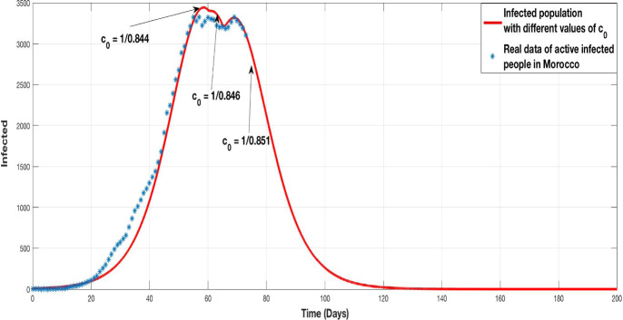
The Fig. 10 shows a comparison between the infected population produced by the model with three phases of $c_0$ (red curve) and the real situation of the active infected people (star-curve $(\ast )$) in Morocco, see [16].

Fig. 10.

Evolution of infected population with three phases of home containment (red curve). Evolution of the real active infected population (star curve)

The real situation is very close to the simulation predicted by the model with three phases of home containment. By bringing together the real data of active infected population and the simulation results of the model, it appears that the Moroccan situation goes through three values of the coefficient of containment control $c_0={\displaystyle \frac{1}{0.844}}$, $c_0={\displaystyle \frac{1}{0.846}}$ and $c_0={\displaystyle \frac{1}{0.851}}$.

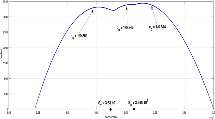
Figure 11 presents the diagram phase of the susceptible/infected population in the case of three phases home containment. Comparing this curve with that of the Fig. 9 ($c_0={\displaystyle \frac{1}{0.844}}$), we show that the new curve has three local maximums, describing the change of the infection rate, instead one global maximum.

Fig. 11.

Diagram phase susceptible/infected population (S, I) with different values of the control containment coefficient $c_0$

Let us analyze the basic reproduction numbers of $S_7^{\ast }=3.63·{10}^7$ and $S_8^{\ast }=3.645·{10}^7$.

Firstly, we have

$$\begin{array}{c}\hfill {\overline{\mathcal{R}}}_0(S_7^{\ast })=1.1773\end{array}$$

and

$$\begin{array}{c}\hfill {\overline{\mathcal{R}}}_0(S_8^{\ast })=1.1822.\end{array}$$

Now for $c_0={\displaystyle \frac{1}{0.844}}$ we get

$$\begin{array}{c}\hfill {\mathcal{R}}_0(c_0,S_7^{\ast })=0.9936\end{array}$$

and

$$\begin{array}{c}\hfill {\mathcal{R}}_0(c_0,S_8^{\ast })=0.9977,\end{array}$$

so these (DFE) are stable for the one phase home containment as shown in Fig. 9, since the curve decreases at these points. This fact is consistent with the condition (5)

$$\begin{array}{c}\hfill {\displaystyle \frac{1}{0.844}}=1.1848>{\overline{\mathcal{R}}}_0(S_7^{\ast })=1.1773\end{array}$$

and

$$\begin{array}{c}\hfill {\displaystyle \frac{1}{0.844}}=1.1848>{\overline{\mathcal{R}}}_0(S_8^{\ast })=1.1822\end{array}$$

Otherwise, for the three phases home containment, $S_7^{\ast }=3.63·{10}^7$ corresponds to $c_0={\displaystyle \frac{1}{0.851}}$ and $S_8^{\ast }=3.645·{10}^7$ corresponds to $c_0={\displaystyle \frac{1}{0.846}}$.

Hence

$$\begin{array}{c}\hfill {\mathcal{R}}_0\left({\displaystyle \frac{1}{0.851}},,,S_7^{\ast }\right)=1.0019\end{array}$$

and

$$\begin{array}{c}\hfill {\mathcal{R}}_0\left({\displaystyle \frac{1}{0.846}},,,S_8^{\ast }\right)=1.0001.\end{array}$$

It follows that these points are unstable as confirmed by the condition (5), since

$$\begin{array}{c}\hfill {\displaystyle \frac{1}{0.851}}=1.1750\ngtr {\overline{\mathcal{R}}}_0(S_7^{\ast })=1.1773\end{array}$$

and

$$\begin{array}{c}\hfill {\displaystyle \frac{1}{0.846}}=1.1820\ngtr {\overline{\mathcal{R}}}_0(S_8^{\ast })=1.1822.\end{array}$$

Conclusion

In this work, a (SIAQRD) was built, integrating asymptomatic people and the isolation of infected person, the quarantine of contacting people and the home containment of all population, strategies. It is established by theoretical investigation and illustrated by simulations that the level of containment is very important to prevent the disease spreading in the absence of vaccine. Several scenarios are tested with different values of the containment control coefficient $c_0$. A relation between the basic reproduction number and $c_0$ was carried out, showing that, a home containment not suitably practiced may lead to a persistence of the pandemic beyond the provided period.

However, we know that the information on the evolution of the pandemic depends on various factors, as the number of tests, which vary considerably each day, detection of person who contacting an infected people,... So, without full data on the real evolution of the pandemic, especially for asymptomatic infected people, it is very hard to estimate parameters, our contribution on the estimation of them is an assignment that must be performed in the next work. Secondly, the choice of containment control values are made theoretically, and it is shown that some values coincide with the real situation in Morocco, it will be interesting to correlate these values with a percentage of the quality of the home containment level, obviously with an important work on the quantification of the confinement.

Compliance with ethical standards

Conflict of interest

The authors declare that they have no conflict of interest.

References

- 1.Anderson M. Population biology of infectious diseases: part 1. Nature. 1979;280:361–367. doi: 10.1038/280361a0. [DOI] [PubMed] [Google Scholar]
- 2.Coronavirus: Common symptoms, preventive measures, & how to diagnose it. https://www.caringlyyours.com/coronavirus, Caringly Yours (2020). Accessed 28 Jan 2020
- 3.Chavez, C.C., Feng, Z., Huang, W.: On the computation of and its role on global stability. Electron. BU-1553-M, (2002). 10.1007/978-1-4757-3667-0-13
- 4.Chisholm RH, Campbell PT, Wu Y, Tong SYC, McVernon J, Geard N. Implications of asymptomatic carriers for infectious disease transmission and control. R. Soc. Open Sci. 2018;5:172341. doi: 10.1098/rsos.172341. [DOI] [PMC free article] [PubMed] [Google Scholar]
- 5.De la Sen M, Ibeas A, Alonso-Quesada S, Nistal R. On a new epidemic model with asymptomatic and dead-infective subpopulations with feedback controls useful for ebola disease. Discrete Dyn. Nat. Soc. 2017 doi: 10.1155/2017/4232971. [DOI] [Google Scholar]
- 6.Diekmann O, Heesterbeek JAP, Metz JAJ. On the definition and the computation of the basic reproduction ratio in models for infectious diseases in heterogeneous populations. J. Math. Biol. 1990;28:365–382. doi: 10.1007/BF00178324. [DOI] [PubMed] [Google Scholar]
- 7.Driessche PVD, Watmough J. Reproduction numbers and sub-threshold endemic equilibria for compartmental models of disease transmission. Math. Biosci. 2002;180(1):29–48. doi: 10.1016/S0025-5564(02)00108-6. [DOI] [PubMed] [Google Scholar]
- 8.Hamer WH. The Milroy Lectures on Epidemic Disease in England: The Evidence of Variability and of Persistency of Type. Lambertville: Bedford Press; 1906. [Google Scholar]
- 9.Hethcote HW. Mathematics of infectious diseases. SIAM Rev. 2000;42(4):599–653. doi: 10.1137/S0036144500371907. [DOI] [Google Scholar]
- 10.Ivorra, B., Ferrández, M.R., Vela-Pérez, M., Ramos, A.M.: Mathematical modeling of the spread of the coronavirus disease 2019 (COVID-19) taking into account the undetected infections. The case of China, Instituto de Matemática Interdisciplinar (IMI) (2020). 10.13140/RG.2.2.21543.29604 [DOI] [PMC free article] [PubMed]
- 11.Jia J, Ding J, Liu S, Liao G, Li J, Duan B, Wang G, Zhang R. Modeling the control of covid-19: impact of policy interventions and meteorological factors. Electron. J. Differ. Equ. 2020;2020(23):1–24. [Google Scholar]
- 12.Jia, J., Ding, J., Liu, S., Liao, G., Li, J., Duan, B., Wang, G., Zhang, R.: Mathematical modeling and epidemic prediction of COVID-19 and its significance to epidemic prevention and control Measures. Ann. Infect. Dis. Epidemiol. 5(1), Art. 1052. (2020)
- 13.Kermack WO, McKendrick AG. A contribution to the mathematical theory of epidemics. Proc. R. Soc. Lond. A Math. Phys. Eng. Sci. 1927;115:700–721. [Google Scholar]
- 14.Kucharski AJ, Russell TW, Diamond C, Liu Y, Edmunds J, Funk S, Eggo RM. Early dynamics of transmission and control of COVID-19: a mathematical modelling study. Lancet Public Health J. 2020 doi: 10.1016/S1473-3099(20)30144-4. [DOI] [PMC free article] [PubMed] [Google Scholar]
- 15.Leung KY, Trapman P, Britton T. Who is the infector? Epidemic models with symptomatic and asymptomatic cases. Math. Biosci. 2018;301:190–198. doi: 10.1016/j.mbs.2018.04.002. [DOI] [PubMed] [Google Scholar]
- 16.Moroccan Healthy Ministry homepage. http://www.covidmaroc.ma/; https://www.sante.gov.ma. Accessed 2020
- 17.Media24 homepage. https://www.medias24.com/covid-19-le-r0-marocain-est-tombe-a-1-18-modele-americain-9650.html. Accessed 21 Apr 2020
- 18.Perasso A. An introduction to the basic reproduction number in mathematical epidemiology. ESAIM Proc. Surv. 2018;62:123–138. doi: 10.1051/proc/201862123. [DOI] [Google Scholar]
- 19.Perra N, Balcan D, Gonçalves B, Vespignani A. Towards a characterization of behavior-disease models. PLoS One J. 2011;6(8):e23084. doi: 10.1371/journal.pone.0023084. [DOI] [PMC free article] [PubMed] [Google Scholar]
- 20.Prem K, Liu Y, Russell TW, Kucharski AJ, Eggo RM, Davies N, Jit M, Klepac P. The effect of control strategies to reduce social mixing on outcomes of the COVID-19 epidemic in Wuhan, China. Lancet Public Health J. 2020 doi: 10.1016/S2468-2667(20)30073-6. [DOI] [PMC free article] [PubMed] [Google Scholar]
- 21.Ross R. The Prevention of Malaria. London: John Murray; 1911. [Google Scholar]
- 22.Safi MA, Gumel AB. Mathematical analysis of a disease transmission model with quarantine, isolation and an imperfect vaccine. Comput. Math. Appl. 2011;61(10):3044–3070. doi: 10.1016/j.camwa.2011.03.095. [DOI] [Google Scholar]
- 23.Sputniknews homepage. https://fr.sputniknews.com/international/202002271043140381-combien-de-personnes-un-porteur-du-coronavirus-peut-il-contaminer/. Accessed 27 Feb 2020
- 24.Tang Y, Xiao D, Zhang W, Zhu D. Dynamics of epidemic models with asymptomatic infection and seasonal successions. Math. Biosci. Eng. 2017;14(5&6):1407–1424. doi: 10.3934/mbe.2017073. [DOI] [PubMed] [Google Scholar]
- 25.Thieme HR. Mathematics in Population Biology. Princeton: Princeton University Press; 2003. [Google Scholar]
- 26.World healthy organization homepage. https://www.who.int/fr/emergencies/diseases/novel-coronavirus-2019/advice-for-public/q-a-coronaviruses. Accessed 2020
- 27.Zeb A, Alzahrani E, Erturk VS, Zaman G. Mathematical model for coronavirus disease: (COVID-19) containing isolation class. BioMed Res. Int. 2019;2020:1. doi: 10.1155/2020/3452402. [DOI] [PMC free article] [PubMed] [Google Scholar]