Motor Cortex Mapping using Active Gaussian Processes

Abstract

One important application of transcranial magnetic stimulation (TMS) is to map cortical motor topography by spatially sampling the motor cortex, and recording motor evoked potentials (MEP) with surface electromyography. Standard approaches to TMS mapping involve repetitive stimulations at different loci spaced on a (typically 1 cm) grid on the scalp. These mappings strategies are time consuming and responsive sites are typically sparse. Furthermore, the long time scale prevents measurement of transient cortical changes, and is poorly tolerated in clinical populations. An alternative approach involves using the TMS mapper expertise to exploit the map’s sparsity through the use of feedback of MEPs to decide which loci to stimulate. In this investigation, we propose a novel active learning method to automatically infer optimal future stimulus loci in place of user expertise. Specifically, we propose an active Gaussian Process (GP) strategy with loci selection criteria such as entropy and mutual information (MI). The proposed method twists the usual entropy- and MI-based selection criteria by modeling the estimated MEP field, i.e., the GP mean, as a Gaussian random variable itself. By doing so, we include MEP amplitudes in the loci selection criteria which would be otherwise completely independent of the MEP values. Experimental results using real data shows that the proposed strategy can greatly outperform competing methods when the MEP variations are mostly conned in a sub-region of the space.

1. INTRODUCTION

Transcranial magnetic stimulation (TMS), provides a non-invasive causal probe of human cortical function. A strong magnetic field applied to the scalp induces an electric field (E-field) within the brain, which at sufficient intensity may result in suprathreshold depolarization of spatially selective cortical neuronal populations and a macroscopic physiological response [21]. TMS can be used for mapping muscle topography by spatially sampling the motor cortex, and recording motor evoked potentials (MEP) [25] using electromyography (EMG). Changes in motor topography assessed with TMS have been associated with changes in function post stroke, highlighting the potential of this technique for elucidating biomarkers of recovery [19].

Traditionally, data acquisition has involved a time consuming process in which repetitive stimuli are delivered at loci on a predefined grid [23], limiting it’s use for clinical assessment. Recently, our group has shown that more efficient mapping can be performed using user-guided selection of stimulation loci based on real time feedback of MEP responses [26, 27]. This strategy, however, still requires relatively extensive sessions and, more importantly, human expertise in order to create reliable maps. In this contribution, we aim at reducing the time and expertise needed to create reliable motor cortex MEP maps by selecting stimulus loci using active machine learning strategies.

In the context of machine learning, active learning consists of a family of strategies in which learning algorithms take action in selecting procedures or making queries that influence what data are added to its training set [3]. Active learning for field estimation finds correlates in different applications such as optimal sensor placement [8, 18], active Gaussian processes [9], weather forecast [4], kriging [6], brain computer interfaces [17], among others. In most of the above-mentioned studies smooth regression strategies based on stochastic formulations, more specifically Gaussian Processes (GPs), are naturally coped with information-based criteria (Entropy and Mutual information) for (near-) optimal location selection [16, 20]. Although such strategies are successful in reducing uncertainty and providing smooth estimation across the entire spatial domain, they may wast valuable time and resources when the field of interest is conned in a small region of the space. The reasoning for this behavior is due to the fact that the GP’s covariance depends exclusively on the selected location points neglecting the information provided by the measurements taken at these locations. For TMS mapping active learning is a surrogate for human expertise when the objective is to optimally select loci and respective MEP measurements used to learn MEP spatial fields. Therefore, accounting for the amplitude of the measurement is critical.

Our specific objective here is to find the excitation area (region of interest) and stimulate in that region. To this aim, we designed an alternative approach to traditional active learning that takes into account the variations of the function to predict optimal future stimulus loci. This new design led to an iterative algorithm that alternates between the GP characterization of the MEP field and loci selection using entropy and mutual information criteria. Differently from previous works which directly considered Gaussian distribution provided by the GP for computing the entropy or MI, here, we model the GP mean as a Gaussian random variable and construct our loci selection criteria based on this random variable. The resulting algorithm provides results that are much closer to expert user-guided mapping strategies, and are faster and more accurate than are given by traditional active GP strategies [18]. Simulations with real data was performed to assess the main characteristics of the proposed method.

This paper is organized as follows. Section 2 briefly presents the TMS Mapping Procedure. Section 3 presents a general discussion about Gaussian Process Regression. Section 4 presents the proposed active sampling methodology. Experimental results are presented in Section 5 and final discussion and future work are discussed in section 6.

2. TRANSCRANIAL MAGNETIC STIMULATION MAPPING PROCEDURE

TMS mapping was conducted on a single healthy right handed subject (male, 34 years old) following IRB approved informed consent and screening for contraindications to TMS. TMS mapping procedures have been previous published elsewhere [26, 27]. Briefly, the subject was seated with the right arm, hand, and fingers comfortably secured in a brace to limit motion. Surface electromyographic activity (EMG, Delsys Trigno, 2kHz) was used to record motor evoked potentials (MEPs), quantified as the peak-to-peak amplitude 20–50ms after the TMS pulse (Figure 1b), from the first dorsal interosseus [FDI] of the right hand. All TMS (Magstim Rapid2, 70mm double coil) stimuli were delivered to the left sensorimotor area. To assure spatial TMS precision the subject’s head was coregistered to a high-resolution anatomical MRI for frameless neuronavigation (Advanced Neuro Technology). The TMS coil was held tangential to the scalp with the handle posterior 45° off the sagittal plane. Following determination of the hotspot the FDI resting motor threshold (RMT) was calculated as the minimum intensity required to elicit MEPs > 50μV in the FDI muscle on 50% of 6 consecutive trials. All mapping was performed with the subject at rest and stimulation intensity set to 110% of the determined RMT. During mapping the TMS operator choose the 294 stimulus loci at their discretion, based on live feedback of MEP amplitude and shape with the goal to maximize the information obtained by increasing the density of points in excitable and border regions while placing very few points in null-response areas (Figure 1a) [27].

Figure 1:

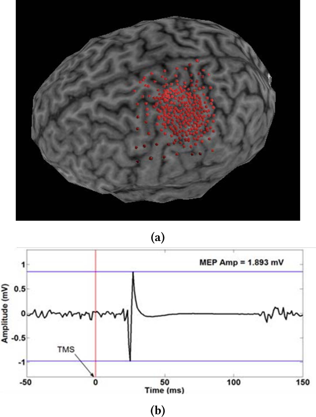
A graphical depiction of the analysis of MEP maps: (a) User points on the brain. (b) MEP signal and peak-to-peak amplitude

3. GAUSSIAN PROCESS FOR TMS MAPPING

Gaussian process (GP) regression methods consist of dening stochastic models for functions and performing inference in functional spaces [24]. These methods have been shown to be useful in a wide variety of fields and tasks including regression and classification [24], detection [11, 12], unmixing [10], and Bayesian optimization [7], to name but a few. This section briefly presents the standard Gaussian process regression [24]. Given a set of N input-output pairs ${\left\{x_k,y_k\right\}}_{k=1}^N$, $x\in \mathcal{X}\subset {ℝ}^d$, y ∈ ℝ related according to an arbitrary model such as

$$y_k=\psi \left(x_k\right)+{\eta }_k$$ (1)

with $\eta ~\mathcal{N}\left(0,{\sigma }_{\eta }^2\right)$, and $\psi \in \mathcal{H}$ considered to be a function of a reproducing kernel Hilbert space $\mathcal{H}$ defined over a compact set $\mathcal{X}$, GPs assume a Gaussian functional distribution as prior for the function $\psi \mid x_k~\mathcal{N}\left(0,\kappa \left(x_k,x_k\right)\right)$, where κ is a kernel function such that $\kappa (\cdot ,x)\in \mathcal{H}$. For a set of input points X = [x₁, …, x_N] the prior distribution for ѱ becomes $\psi \mid X~\mathcal{N}(0,K)$, where K ∈ ℝ^N×N is the Gram matrix with entries [K]_ij = κ(x_i, x_j) For a given set of measurements y = [y₁, …,y_N]^⊤ associated with the positions X, the prior distribution becomes

$$y~\mathcal{N}\left(0,K+{\sigma }_{\eta }^{2}I\right).$$ (2)

The predictive distribution allows one to “predict” the value of the function ѱ_★ for a new input value x_★. Thus, we have ${\psi }_{\star }\mid x_{\star }~\mathcal{N}\left(0,{\kappa }_{\star \star }\right)$, where ${\kappa }_{\star \star }\triangleq \kappa \left(x_{\star },x_{\star }\right)$. Since y and ѱ_★ are jointly Gaussian their joint PDF is given by

$$\left(\begin{array}{c}y\\ {\psi }_{\star }\end{array}\right)~N\left(0,\left(\begin{array}{cc}K+{\sigma }_{\eta }^{2}I& {\kappa }_{\star }\\ {\kappa }_{\star }^{\top }& {\kappa }_{\star \star }\end{array}\right)\right),$$ (3)

where ${\kappa }_{\star }\triangleq {\left[\kappa \left(x_1,x_{\star }\right),\dots ,\kappa \left(x_N,x_{\star }\right)\right]}^{\top }$. Finally the predictive distribution can be obtained by conditioning ѱ_★ over the observation and the its respective positions as

$${\psi }_{\star }\mid y,X,x_{\star }~\mathcal{N}\left({\widehat{\psi }}_{\star },s_{\star }^2\right)$$ (4)

with ${\widehat{\psi }}_{\star }={\kappa }_{\star }^{\top }{\left(K+{\sigma }_{\eta }^{2}I\right)}^{-1}y$, and $s_{\star }^2={\kappa }_{\star \star }-{\kappa }_{\star }^{\top }{\left(K+{\sigma }_{\eta }^{2}I\right)}^{-1}{\kappa }_{\star }$.

The Bayesian framework also provides strategies to estimate free parameters, such as the kernel parameters θ and the noise power ${\sigma }_{\eta }^2$. The classical approach [24] aims at maximizing the marginal likelihood $p\left(y\mid X,{\sigma }_{\eta }^2,\theta \right)$ with respect to $\left({\sigma }_{\eta }^2,\theta \right)$.

4. ACTIVE SAMPLE SELECTION

Active sample selection finds correlates in many fields and applications such as Optimal Sensor placement [8, 18], Active Gaussian processes [9], weather forecast [4], etc. In most scenarios the problem is often stated as given a set of input-output pairs (x_ℓ, y_ℓ), $\mathcal{l}\in \mathcal{V}$, $\mathcal{V}$ being the index set of all possible data pairs, select a subset $\mathcal{A}\subset \mathcal{V}$, with cardinality $\left|\mathcal{A}\right|=n_{\mathcal{A}}\ll \left|\mathcal{V}\right|=n_{\mathcal{V}}$, which can be obtained using some optimality criterion.

The literature presents near-optimal strategies that are often based on information theoretic criteria to select appropriate data samples. This copes very well with GPs since GPs provides a proper stochastic framework which can be exploit to compute the desired criteria [18, 22]. In [8, 18, 22] optimal point selection strategies are presented in conjunction with GPs. In these works, the authors consider entropy- and mutual information-based criteria to provide a greedy near-optimal strategy which boils down to analyze the variances provided by the GP. Although these strategies succeeded in reducing GP uncertainty across the space, the variances provided by the GP depend exclusively on the location points x_κ neglecting completely information regarding field variations. This implies that even if the mapped field presents variations conned into a specific region, such methodologies will lead to evenly (depending on the kernel selected) sampling the entire space what can lead to lost of resolution in the region of interest.

To circumvent this issue, we propose here an alternative approach that takes into account the variations of the function ψ and that are much closer to expert human mapping strategies. We use the GP estimation (i.e., the GP mean) $\widehat{\psi }$ to construct an iterative strategy where GP estimation and sample selection are performed sequentially.

Thus, given an index set $\mathcal{A}$ with respective sample pairs $\left(X_{\mathcal{A}},y_{\mathcal{A}}\right)$ the GP estimation ${\widehat{\psi }}_{p\in \mathcal{V}}$ can be obtained by taking the mean of (4). Assuming a zero-mean Gaussian prior for ${\widehat{\psi }}_p$ with covariance κ(∙,∙) we have

$${\widehat{\psi }}_p~\mathcal{N}\left(0,{\kappa }_{pp}\right)$$ (5)

with ${\kappa }_{\mathit{p}\mathit{p}}\triangleq \kappa \left({\widehat{\psi }}_{\mathit{p}},{\widehat{\psi }}_{\mathit{p}}\right)$ and the MEP field at selected indices ${\widehat{\psi }}_{\mathcal{A}}$ is distributed

$${\widehat{\psi }}_{\mathcal{A}}~\mathcal{N}\left(0,K_{\mathcal{A}\mathcal{A}}\right)$$ (6)

with $K_{\mathcal{A}\mathcal{A}}\triangleq \kappa \left({\widehat{\psi }}_{\mathcal{A}},{\widehat{\psi }}_{\mathcal{A}}\right)$. Now, consider a sample ${\widehat{\psi }}_{\mathcal{l}}$, $\mathcal{l}\in {\mathcal{V}}_{\backslash \mathcal{A}}$, the joint distribution of ${\widehat{\psi }}_{\mathcal{l}}$ and ${\widehat{\psi }}_{\mathcal{A}}$ is given by

$$\left(\begin{array}{c}{\widehat{\psi }}_{\mathcal{A}}\\ {\widehat{\psi }}_{\mathcal{l}}\end{array}\right)~\mathcal{N}(0,\left(\begin{array}{cc}{K}_{\mathcal{A}\mathcal{A}}& {\kappa }_{\mathcal{A}\mathcal{l}}\\ {\kappa }_{\mathcal{A}\mathcal{l}}^{\top }& {\kappa }_{\mathcal{l}\mathcal{l}}\end{array}\right),$$ (7)

with ${\kappa }_{\mathcal{A}\mathcal{l}}\triangleq {\left[\kappa \left({\widehat{\psi }}_{{\mathcal{A}}_1},{\widehat{\psi }}_{\mathcal{l}}\right),\dots ,\kappa \left({\widehat{\psi }}_{{\mathcal{A}}_{n_{\mathcal{A}}}},{\widehat{\psi }}_{\mathcal{l}}\right)\right]}^{\top }$. Using the identity in [1, pg. 87] we have

$${\widehat{\psi }}_{\mathcal{l}}\mid {\widehat{\psi }}_{\mathcal{A}}~\mathcal{N}\left({\mu }_{{\widehat{\psi }}_{\mathcal{l}\mid \mathcal{A}}},{\sigma }_{{\widehat{\psi }}_{\mathcal{l}\mid \mathcal{A}}}^2\right)$$ (8)

with

$${\mu }_{{\widehat{\psi }}_{\mathcal{l}\mid \mathcal{A}}}={\kappa }_{\mathcal{A}\mathcal{l}}^{\top }{K}_{\mathcal{A}\mathcal{A}}^{-1}{\psi }_{\mathcal{A}}$$ (9)

$${\sigma }_{{\widehat{\psi }}_{\mathcal{l}\mid \mathcal{A}}}^2={\kappa }_{\mathcal{l}\mathcal{l}}-{\kappa }_{\mathcal{A}\mathcal{l}}^{\top }{K}_{\mathcal{A}\mathcal{A}}^{-1}{\kappa }_{\mathcal{A}\mathcal{l}}.$$ (10)

Next we present the entropy and MI resulting problems.

4.1. Grid Entropy Criterion

The goal of active learning for our use case is to select future stimulus locations which are most informative with respect to the entire grid of possible sampling locations. As said, a good conception of uncertainty is the conditional entropy when we consider finite subsets $\mathcal{A}$ of measured locations and $\mathcal{V}$ all other possible locations. We can define conditional entropy of the available measurement locations $\mathcal{V}\backslash \mathcal{A}$ after $\mathcal{A}$ measured locations,

$$H\left({\widehat{\psi }}_{{\mathcal{V}}_{\backslash \mathcal{A}}}\mid {\widehat{\psi }}_{\mathcal{A}}\right)=-\int p\left({\widehat{\psi }}_{{\mathcal{V}}_{\backslash \mathcal{A}}},{\widehat{\psi }}_{\mathcal{A}}\right)\text{log}p\left({\widehat{\psi }}_{{\mathcal{V}}_{\backslash \mathcal{A}}}|{\widehat{\psi }}_{\mathcal{A}}\right)d{\widehat{\psi }}_{{\mathcal{V}}_{\backslash \mathcal{A}}}d{\widehat{\psi }}_{\mathcal{A}}.$$ (11)

Thus, an informative set of measurements would minimize this conditional entropy leading to an optimization problem known to be NP-Complete [15]. To minimize this issue the literature presents greedy heuristics in which starting with an initial set ${\mathcal{A}}_0$, $\left|{\mathcal{A}}_0\right|=n_{{\mathcal{A}}_0}<n_{\mathcal{A}}$, the algorithm greedily adds new samples until the desired cardinality $n_{\mathcal{A}}$ is achieved [18]. In such approaches at each iteration the index ℓ maximizing the conditional entropy $H\left({\widehat{\psi }}_{\mathcal{l}}\mid {\widehat{\psi }}_{\mathcal{A}}\right)$ should be selected, leading to

$${\mathcal{l}}^{*}=\underset{\mathcal{l}\in {\mathcal{V}}_{\backslash \mathcal{A}}}{\text{arg}\text{max}}H\left({\widehat{\psi }}_{\mathcal{l}}\mid {\widehat{\psi }}_{\mathcal{A}}\right)$$ (12)

where ℓ is a index not in $\mathcal{A}$. The conditional entropy for Gaussian random variables is well known and given by [5]

$$H\left({\widehat{\psi }}_{\mathcal{l}}\mid {\widehat{\psi }}_{\mathcal{A}}\right)=\frac{1}{2}\text{log}\left(2\pi e{\sigma }_{{\widehat{\psi }}_{\mathcal{l}\mid \mathcal{A}}}^2\right)$$ (13)

leading to a simple and effective selection strategy. Since log (ζ) is monotonically increasing for ζ ∈ ℝ₊, problem (12) can be solved by finding the sample index $\mathcal{l}\in {\mathcal{V}}_{\backslash \mathcal{A}}$, that maximizes the quantity

$${\delta }_{\psi ,\mathcal{l}}^{\text{Entropy }}={\sigma }_{{\widehat{\psi }}_{\mathcal{l}\mid \mathcal{A}}}^2={\kappa }_{\mathcal{l}\mathcal{l}}-{\kappa }_{\mathcal{A}\mathcal{l}}^{\top }{K}_{\mathcal{A}\mathcal{A}}^{-1}{\kappa }_{\mathcal{A}\mathcal{l}}.$$ (14)

4.2. Mutual Information

A known issue with the entropy criterion discussed above is the tendency to select loci along the edges of the sample space. This issue can be understood by the fact that the entropy grid approach aims at selecting the ${\widehat{\psi }}_{\mathcal{l}}$ with largest variance ${\sigma }_{{\widehat{\psi }}_{\mathcal{l}\mid \mathcal{A}}}$. These uncertainties are known to be larger in the edges of the sampling space specially when more flexible interpolation methods are considered [13].

An alternative approach, proposed by Caselton and Zidek [2], is based on the mutual information (MI) of random variables within the set $\mathcal{A}$ and in ${\mathcal{V}}_{\backslash \mathcal{A}}$. This strategy leads to an optimization criterion that searches for the subset of locations that most significantly reduce the uncertainty about the estimates in the rest of the space [18]. Different from the entropy, the MI criterion tends to find loci that are most informative about the unstimulated locations. The resulting optimization problem aims at maximizing the mutual information $I\left({\widehat{\psi }}_{{\mathcal{V}}_{\backslash \mathcal{A}}};{\widehat{\psi }}_{\mathcal{A}}\right)=H\left({\widehat{\psi }}_{{\mathcal{V}}_{\backslash \mathcal{A}}}\right)-H\left({\widehat{\psi }}_{{\mathcal{V}}_{\backslash \mathcal{A}}}\mid {\widehat{\psi }}_{\mathcal{A}}\right)$ and can be also shown to be NP-Complete.

In [18], a greedy approximation algorithm was presented which reduces to select the next sampling point that provides the maximum increase in mutual information $I\left({\widehat{\psi }}_{{\mathcal{V}}_{\backslash \mathcal{A}}};{\widehat{\psi }}_{\mathcal{A}}\right)$.

Krause described an approximation for maximizing mutual information [18] which led to a greedy algorithm. The idea is to at each iteration select the location that provides the maximum increase in mutual information. Thus, at each iteration the goal is to greedily select the location index $\mathcal{l}\in \mathcal{V}$ that maximizes

$$\begin{gathered} I\left({\widehat{\psi }}_{{\mathcal{V}}_{\mathcal{A}\cup \mathcal{l}}};{\widehat{\psi }}_{\mathcal{A}\cup \mathcal{l}}\right)-I\left({\widehat{\psi }}_{{\mathcal{V}}_{\backslash \mathcal{A}}};{\widehat{\psi }}_{\mathcal{A}}\right) \\ =H\left({\widehat{\psi }}_{\mathcal{l}}\mid {\widehat{\psi }}_{\mathcal{A}}\right)-H\left({\widehat{\psi }}_{\mathcal{l}}\mid {\widehat{\psi }}_{{\mathcal{V}}_{\backslash \mathcal{A}}}\right) \\ =\text{log}\left({\sigma }_{{\widehat{\psi }}_{\mathcal{l}\mid \mathcal{A}}}^2\right)-\text{log}\left({\sigma }_{{\widehat{\psi }}_{\mathcal{l}}\mid {\mathcal{V}}_{\backslash \mathcal{A}}}^2\right)+\text{cte} \end{gathered}$$ (15)

where cte is a constant.

This leads to selecting a location that provides the largest variance ratio

$${\delta }_{\psi ,\mathcal{l}}^{\text{MI}}=\frac{{\kappa }_{\mathcal{l}\mathcal{l}}-{\kappa }_{\mathcal{A}\mathcal{l}}^{\top }{K}_{\mathcal{A}\mathcal{A}}^{-1}{\kappa }_{\mathcal{A}\mathcal{l}}}{{\kappa }_{\mathcal{l}\mathcal{l}}-{\kappa }_{\overline{\mathcal{A}}\mathcal{l}}^{\top }{K}_{\overline{\mathcal{A}}\overline{\mathcal{A}}}^{-1}{\kappa }_{\overline{\mathcal{A}}\mathcal{l}}}$$ (16)

where $\overline{\mathcal{A}}={\mathcal{V}}_{\mathcal{A}\cup \mathcal{l}}$.

4.3. The sampling algorithm

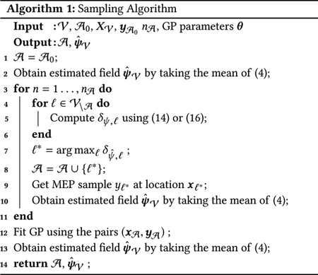
The proposed iterative methodology is summarized in Algorithm 1. It is designed to work with a set of selectable points $\mathcal{V}$ and assumes prior knowledge of the kernel parameters θ, Besides $\mathcal{V}$ and θ, the inputs of Algorithm 1 are the initial index set ${\mathcal{A}}_0$ and respective measurements $y_{{\mathcal{A}}_0}$, the set of all possible loci $X_{\mathcal{V}}$ and the final desired cardinality $n_{\mathcal{A}}$. The algorithm follows a iterative sequence interchanging between computing δψ,ℓ for all $\mathcal{l}\in {\mathcal{V}}_{\backslash \mathcal{A}}$ lines 4–6, finding the optimal index (line 7) and MEP field estimation in lines 2 and 10. When a new index ℓ* is selected (line 7) and included in the set of selected indices (line 8) a new measurement, y_ℓ*, is obtained at the respective location x_ℓ* (line 9). When the desired cardinality is achieved the algorithim performs a GP fit (line 12) and. estimation (line 13), and return the set of selected indices $\mathcal{A}$ and the final MEP field estimation ${\widehat{\psi }}_{\mathcal{V}}$ for all set $X_{\mathcal{V}}$.

5. EXPERIMENTS

In this section we present our simulation of experimental results using the active GP for MEP interpolation and TMS mapping for one subject. We compare the methodology proposed in Section 4 using Entropy and MI, namely, Entropyψ and MIψ with the Entropyψ and MI directly using the GP distribution [18], and a Random (uniform) point selection TMS mapping approach.

To assess the performance of the different algorithms we resort to a metric: the normalized mean squared error (NMSE), between the target function and the predicted map. NMSE is given by the formula:

$$\text{NMSE}(\psi ,\widehat{\psi })=\frac{\Vert \psi -\widehat{\psi }{\Vert }_2^2}{\Vert \psi {\Vert }_2^2}$$

where ψ is the vector containing the MEP amplitudes of the target function and $\widehat{\psi }$ is the GP estimation using the set of selected points.

Monte Carlo simulations with n_MC = 100 runs were also performed to assess the mean behavior and standard deviation of the different methods. For all simulations a initial set ${\mathcal{A}}_0$ with cardinality $\left|\mathcal{A}\right|=20$ was selected randomly, and the kernel parameters θ were fixed and assumed to be known a priori.

5.1. Data-set derived from human expert mapping

The experimental dataset was composed of 282 of 293 stimuli obtained from a healthy human participant using a user guided approach. Eleven stimuli were excluded for excessive subject head movement, poor coil placement or voluntary muscle contraction. The data was concatenated and a GP was used to interpolate all available points. Figure 2 presents the resulting GP interpolation in 3D (left) and 2D (right). The black circles in the right panel are the points selected by the human expert.

Figure 2:

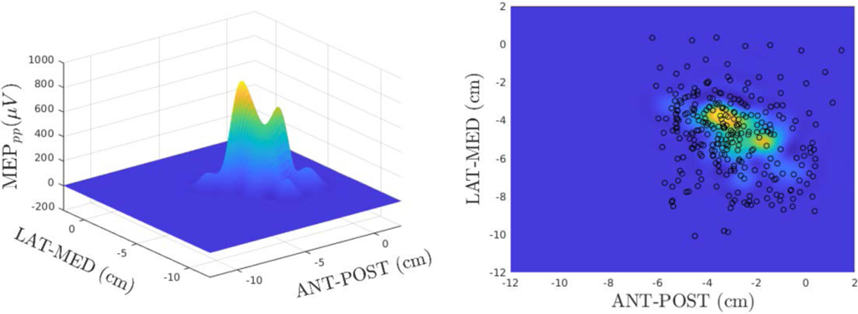
Target function / Expert Human Mapper. X, Y axes represent anterior-posterior and lateral-medial directions, respectively. MEP amplitude is presented in microvolts (μV)on the Z axis.

For all subsequent simulations we used the GP interpolated map of Figure 2 as our target function (ground truth).

5.2. Results

The results discussed in this section are summarized in Figures 3 and 4 and Table 1 for the 5 selected methods. For all 5 methods the nal cardinality was $n_{\mathcal{A}}=282$ including the 20 initial points assumed in ${\mathcal{A}}_0$, that is, a total of 262 new points were selected using each one of the selected methods.

Figure 3:

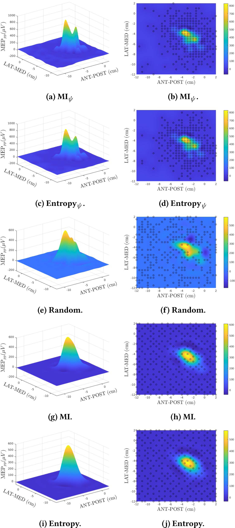
Results comparing different point selection methods.

Figure 4:

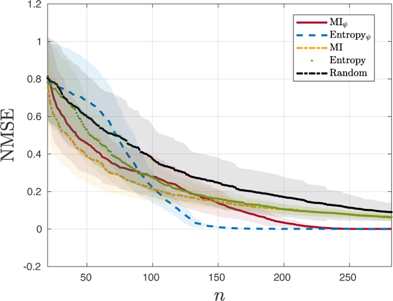
NMSE for test the algorithms (n: number of stimuli).

Table 1:

Final NMSE for predicted map

Method	NMSE
MIψ	0.021 ± 0.006
Entropyψ	0.029 ± 0.003
Random	0.122 ± 0.055
MI	0.119 ± 0.035
Entropy	0.115 ± 0.038

Figure 3 shows the estimated maps and selected points provided by each method. When comparing with the target function, Figure 2, a simple visual inspection shows a clear superiority of the results obtained with MI_ψ (Figure 3a) and Entropy_ψ (Figure 3c) since the resulting maps captured the two main peaks of the cortical topography as well as the smaller side-lobes. This contrasts with the more bell-shaped maps obtained by using the other methodologies. When analyzing the selected points for all methods, the proposed strategies (Figures 3d and 3b) concentrated the selected loci in the region of interest. The reasoning for this behavior follows from the fact that the proposed strategy selects locations based on the GP mean values instead of spatial locations that are uncorrelated with the field amplitude. This also explains the more uniform spread obtained with Entropy and MI in Figures 3d and 3h, respectively. Monte Carlo simulations were also performed and are presented in Figure 4 where the NMSE mean (solid color) and standard deviation (STD) (transparent shade) for the number of samples used is depicted for all 5 methods. The plots show that for all methods the NMSE and the STD decreased as n increases. Although all methods present high STD for n < 100, the MI presents the best average performance followed by MI_ψ. When n > 100, Entropy_ψ outperforms the competing methods presenting both smaller average NMSE and STD, and displaying convergence at n > 150. MI_ψ also converges for n > 230 presenting a comparable average NMSE and STD to the Entropy_ψ and outperforming the other competing methods. The final results for n = 262 are presented in Table 1 showing that the proposed methodology clearly outperformed the competing algorithms and corroborating the conclusions obtained by the visual inspection of Figures 2 and 3.

6. CONCLUSIONS

In this paper we proposed an active GP strategy for TMS mapping. The proposed method modied the usual GP-Entropy/ MI-based selection criteria by modeling the GP mean as a Gaussian random variable. The experiments show that the proposed strategies (MI_ψ and Entropy_ψ) is suitable for localizing and sampling the region of the space containing most of the the fields variation. The results also show a trade-off among the different algorithms. When the number of samples is very small (n < 100) more exploratory strategies (MI, Entropy, and Random) lead to smaller average NMSE. When more samples are available, n > 100 the proposed method (MI_ψ and Entropy_ψ) clearly show better convergence rates and accuracy. Our results indicate that the proposed method was able to mimic user expertise reducing the need for TMS operator training. Reducing the need for expertise in TMS mapping could eliminate a potential barrier to use of TMS mapping of motor topography as biomarker of pathology or to track recovery due to intervention. More widespread use of TMS in this fashion will likely increase our understanding of who may recovery from intervention, thereby increasing the effectiveness of rehabilitation [27]. Recently, several robotic TMS positioning systems have become commercially available [14]. Combining active learning for the selection of stimulus loci during automated TMS mapping of motor topography using robotic positioning would even further reduce barriers of use. Additionally, the proposed Entropy_ψ method was able to achieve maximal accuracy with only ~150 stimulations. At a commonly used inter-stimulus interval of 4 seconds, this means that mapping could be achieved in as little as 10 minutes. This increased efficiency is critical for the use of TMS mapping in populations who may not tolerate prolonged mapping such as individuals in the acute period of recovery from stroke sessions, or for the measurement of transient changes in cortical representations due to intervention. Natural extensions of this work are related to considering methodologies for recursive parameter estimation for GPs allowing for a completely blind strategy, providing theoretical convergence analysis and proposing new sampling criteria that can balance an initial exploratory analysis (such as the one obtained by the MI) with the more region focused criteria such as the proposed strategies.

CCS CONCEPTS.

• Theory of computation → Active learning; Gaussian processes; • Applied computing → Health informatics.

REFERENCES

- [1].Bishop CM. 2006. Pattern recognition and machine learning. springer. [Google Scholar]
- [2].Caselton WF and Zidek JV. 1984. Optimal monitoring network designs. Statistics & Probability Letters 2, 4 (1984), 223–227. [Google Scholar]
- [3].Cohn DA, Ghahramani Z, and Jordan MI. 1996. Active learning with statistical models. Journal of artificial intelligence research 4 (1996), 129–145. [Google Scholar]
- [4].Comboul M, Emile-Geay J, Hakim GJ, and Evans MN. 2015. Paleoclimate sampling as a sensor placement problem. Journal of Climate 28, 19 (2015), 7717–7740. [Google Scholar]
- [5].Cover TM and Thomas JA. 2012. Elements of information theory. John Wiley & Sons. [Google Scholar]
- [6].Echard B, Gayton N, and Lemaire M. 2011. AK-MCS: an active learning reliability method combining Kriging and Monte Carlo simulation. Structural Safety 33, 2 (2011), 145–154. [Google Scholar]
- [7].Frazier PI. 2018. A tutorial on Bayesian optimization. arXiv preprint arXiv:1807.02811 (2018).
- [8].Guenther J and Sawodny O. 2019. Optimal Sensor Placement based on Gaussian Process Regression for Shared Office Spaces under Various Ventilation Conditions In 2019 IEEE International Conference on Systems, Man and Cybernetics (SMC). IEEE, 2883–2888. [Google Scholar]
- [9].Huber MF. 2014. Recursive Gaussian process: On-line regression and learning. Pattern Recognition Letters 45 (2014), 85–91. [Google Scholar]
- [10].Imbiriba T, Bermudez JCM, Richard C, and Tourneret J-Y. 2016. Non-parametric detection of nonlinearly mixed pixels and endmember estimation in hyperspectral images. IEEE Transactions on Image Processing 25, 3 (2016), 1136–1151. [DOI] [PubMed] [Google Scholar]
- [11].Imbiriba T, Bermudez JCM, Tourneret J-Y, and Richard C. 2014. Detection of nonlinear mixtures using Gaussian processes: Application to hyperspectral imaging In 2014 IEEE International Conference on Acoustics, Speech and Signal Processing (ICASSP). IEEE, 7949–7953. [Google Scholar]
- [12].Imbiriba T, LaMountain G, Wu P, and Closas P. 2019. Change detection and Gaussian process inference in piecewise stationary environments under noisy inputs In Proc. of the CAMSAP’19 Guadeloupe, West Indians. [Google Scholar]
- [13].James G, Witten D, Hastie T, and Tibshirani R. 2013. An introduction to statistical learning. Vol. 112 Springer. [Google Scholar]
- [14].Kantelhardt SR, Fadini T, Finke M, Kallenberg K, Siemerkus J, Bocker-mann V, Matthaeus L, Paulus W, Schweikard A, Rohde V, and Giese A. 2010. Robot-assisted image-guided transcranial magnetic stimulation for somatotopic mapping of the motor cortex: a clinical pilot study. Acta neurochirurgica 152, 2 (2010), 333–343. [DOI] [PMC free article] [PubMed] [Google Scholar]
- [15].Ko CW, Lee J, and Queyranne M. 1995. An exact algorithm for maximum entropy sampling. Operations Research 43, 4 (1995), 684–691. [Google Scholar]
- [16].Koçanaoğulları A, Erdoğmuş D, and Akçakaya M. 2018. On analysis of active querying for recursive state estimation. IEEE signal processing letters 25, 6 (2018), 743–747. [DOI] [PMC free article] [PubMed] [Google Scholar]
- [17].Koçanaoğulları A, Marghi YM, Akçakaya M, and Erdoğmuş D. 2020. An active recursive state estimation framework for brain-interfaced typing systems. Brain-Computer Interfaces (2020), 1–13. [Google Scholar]
- [18].Krause A, Singh A, and Guestrin C. 2008. Near-optimal sensor placements in Gaussian processes: Theory, efficient algorithms and empirical studies. Journal of Machine Learning Research 9 (2008), 235–284. [Google Scholar]
- [19].Lüdemann-Podubecká J and Nowak DA. 2016. Mapping cortical hand motor representation using TMS: A method to assess brain plasticity and a surrogate marker for recovery of function after stroke? Neuroscience & Biobehavioral Reviews 69 (2016), 239–251. [DOI] [PubMed] [Google Scholar]
- [20].Nemhauser GL, Wolsey LA, and Fisher ML. 1978. An analysis of approximations for maximizing submodular set functions—I. Mathematical programming 14, 1 (1978), 265–294. [Google Scholar]
- [21].Ruohonen J and Ilmoniemi RJ. 2002. Handbook of TMS. Oxford University Press. [Google Scholar]
- [22].Schulz E, Speekenbrink M, and Krause A. 2018. A tutorial on Gaussian process regression: Modelling, exploring, and exploiting functions. Journal of Mathematical Psychology 85 (2018), 1–16. [Google Scholar]
- [23].Thickbroom GW, Sammut R, and Mastaglia FL. 1998. Magnetic stimulation mapping of motor cortex: factors contributing to map area. Electroencephalography and Clinical Neurophysiology/Electromyography and Motor Control (1998), 79–84. [DOI] [PubMed] [Google Scholar]
- [24].Williams CKI and Rasmussen CE. 2006. Gaussian processes for machine learning. Vol. 2 MIT press; Cambridge, MA. [Google Scholar]
- [25].Wilson SA, Thickbroom GW, and Mastaglia FL. 1993. Transcranial magnetic stimulation mapping of the motor cortex in normal subjects: the representation of two intrinsic hand muscles. Journal of the neurological sciences 118, 2 (1993), 134–144. [DOI] [PubMed] [Google Scholar]
- [26].Yarossi M, Adamovich S, and Tunik E. 2014. Sensorimotor cortex reorganization in subacute and chronic stroke: a neuronavigated TMS study In 2014 36th Annual International Conference of the IEEE Engineering in Medicine and Biology Society. IEEE, 5788–5791. [DOI] [PMC free article] [PubMed] [Google Scholar]
- [27].Yarossi M, Quivira F, Dannhauer M, Sommer MA, Brooks DH, Erdoğmuş D, and Tunik E. 2019. An experimental and computational framework for modeling multi-muscle responses to transcranial magnetic stimulation of the human motor cortex In 2019 9th International IEEE/EMBS Conference on Neural Engineering (NER). IEEE, 1122–1125. [DOI] [PMC free article] [PubMed] [Google Scholar]
Associated Data
This section collects any data citations, data availability statements, or supplementary materials included in this article.