An SEIARD epidemic model for COVID-19 in Mexico: Mathematical analysis and state-level forecast

Highlights

• •An epidemic model with asymptomatic infections is proposed.
• •The basic reproduction number and stability of the model are studied.
• •The parameters are fitted to the reported cases of COVID-19 in Mexico.
• •Temporal forecasts are made for the spread in several states of Mexico.

Abstract

We propose an SEIARD mathematical model to investigate the current outbreak of coronavirus disease (COVID-19) in Mexico. Our model incorporates the asymptomatic infected individuals, who represent the majority of the infected population (with symptoms or not) and could play an important role in spreading the virus without any knowledge. We calculate the basic reproduction number (R₀) via the next-generation matrix method and estimate the per day infection, death and recovery rates. The local stability of the disease-free equilibrium is established in terms of R₀. A sensibility analysis is performed to determine the relative importance of the model parameters to the disease transmission. We calibrate the parameters of the SEIARD model to the reported number of infected cases, fatalities and recovered cases for several states in Mexico by minimizing the sum of squared errors and attempt to forecast the evolution of the outbreak until November 2020.

1. Introduction

At the beginning of December 2019, a new virus caused an increase in atypical pneumonia at the city of Wuhan in China. The virus was isolated, sequenced and identified as a new type of coronavirus [1]. The virus was called SARS-CoV-2 and the disease associated with that virus was called COVID-19 [2]. On March 11, 2020, the World Health Organization (WHO) declared the outbreak of COVID-19 as a global pandemic [3]. Most of the infected individuals will develop a mild respiratory illness and they won’t need any special requirements; they will just need to manage the symptoms. Symptoms associated to COVID-19 are fever, cough and fatigue, few may develop other symptoms like headache and diarrhea, to name some.

The first case of COVID-19 confirmed in Mexico was until February 2020, which was an imported case from Europe, by that time it was an epicenter of the disease. Mexican authorities announced on March 14 the “Jornada Nacional de Sana Distancia” that basically means quarantine for vulnerable groups. Not only elderly individuals are considered a group of risk, also individuals that have co-morbidities like diabetes, hypertension and obesity can develop more complicated respiratory symptoms that can be fatal. Mexico declared phase 2 of the coronavirus pandemic on March 23 with 367 confirmed cases. As of July 16, there were 324 041 confirmed cases and 37 574 deaths. In [4], Cruz-Pacheco et al. estimated the arrival of the infectious outbreak to Mexico between March 20 and March 30, 2020. Other models for predicting the evolution of COVID-19 outbreak in Mexico have been proposed in Alvarez et al. [5], Acuña Zegarra et al. [6].

In this paper, we modify the SIR epidemic model with a novel SEIARD epidemic model. We included a subpopulation of asymptomatic individuals, the so-called hidden cases. Even though in the case of Mexico, there have not been a characterization of the asymptomatic cases, we believe the proportion of this subpopulation is roughly 0.14 based on the estimation of a mathematical model applied in Tang et al. [7].

Compartmental models like the one used in this paper have been used for studying the spread of the COVID-19 pandemic in several countries, such as China [8], [9], [10], Italy [11], [12] and other parts of the world [13], [14], [15]. In this study, we use a compartmental mathematical model to try to understand the outbreak of COVID-19 in Mexico, and we evaluate the heterogeneity of COVID-19 throughout Mexican territory considering two important regions: the Mexico Valley and the Yucatan Peninsula.

The rest of the paper is structured as follows. We formulate the mathematical model, compute the basic reproduction number and perform a sensibility analysis in Section 2. In Section 3, we calibrate our mathematical model using a sum of squared errors approach using daily cumulative of infected, death and recovered individuals published daily by the Ministry of Health in Mexico. We used the data until July 2, 2020. In Section 4, we explore the simulations of the cases in Mexico and compare how different the outbreak is in the two regions. Lastly, we provide some concluding remarks in Section 5.

2. Mathematical model with asymptomatic individuals

In this work, we will use a compartmental differential equation model for the spread of COVID-19 in Mexico. The model monitors the dynamics of six subpopulations, which are: susceptible (S(t)), exposed (E(t)), infected (I(t)), asymptomatic (A(t)), recovered (R(t)) and dead (D(t)).

The model simulations will be carried out with the following assumptions:

• (a)The susceptible and infected individuals are homogeneous in the population.
• (b)At first, no interventions were applied to stop the spread of COVID-19.
• (c)No births are allowed in the population, and we only take into account the fatalities associated to COVID-19.

Fig. 1 shows a diagram of the flow through the compartmental subpopulations.

Fig. 1.

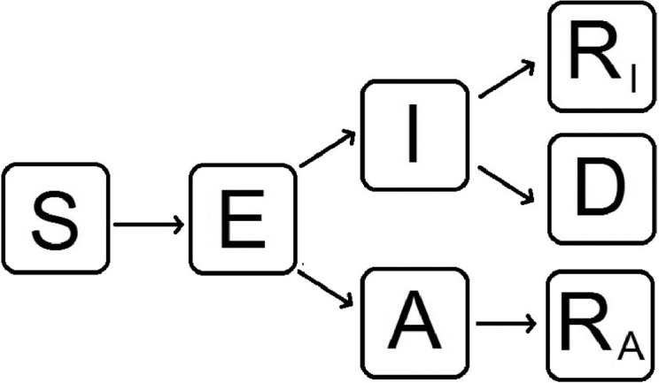
Flow diagram of our mathematical model to evaluate the behavior of the spread of nCoV-2019 in Mexico. S: susceptible, E: exposed, I: infected with symptoms, A: infected but without symptoms (asymptomatic), R_I: recovered from symptomatic infection, R_A: recovered from asymptomatic infection, D: dead.

Susceptible population S(t): This subpopulation cannot increase, because we are not considering any natural recruitments (births) or deaths that are not related to COVID-19. The susceptible population will only decrease after an infection, an acquired characteristic due to the interaction with an infected person or asymptomatic one. The transmission coefficients will be βI and βA. The rate of change of the susceptible population is expressed in the following equation:

$$\frac{\text{d}S}{\text{d}t}=-\beta S\left(\frac{I+A}{N-D}\right).$$ (1)

Exposed population E(t): Because we are modeling an infectious disease caused by a virus, we included the exposed population to mimic the latent period, which is the period between the infection with the virus and the moment when the host is able to transmit the pathogen to susceptible individuals. The exposed subpopulation consists of individuals that are infected but not infectious, i.e., they cannot infect others. This population decreases at a rate w to become infectious with or without symptoms. The parameter 1/w denotes the average length of the latent period; hence, after 1/w time units, an exposed individual becomes symptomatically infectious with a probability p or asymptomatically infectious with a probability $1-p$. Consequently,

$$\frac{\text{d}E}{\text{d}t}=\beta S\left(\frac{I+A}{N-D}\right)-wE=\beta S\left(\frac{I+A}{N-D}\right)-pwE-(1-p)wE.$$ (2)

Infected population I(t): Infected (symptomatic) individuals are generated at a proportion p ∈ (0, 1) from the exposed class. They recover at a rate γ and die at a rate δ. This is the only population that acknowledges death. Thus,

$$\frac{\text{d}I}{\text{d}t}=pwE-(\delta +\gamma )I.$$ (3)

Asymptomatic population A(t): This population is considered an infected population, but the individuals do not develop the common symptoms of COVID-19. Asymptomatic individuals are important to model because they have the ability to spread the virus without knowing; they are produced at a proportion $1-p$ from the exposed class and recover at a rate γ. Consequently,

$$\frac{\text{d}A}{\text{d}t}=(1-p)wE-\gamma A.$$ (4)

Recovered populations R_I(t) and R_A(t): All individuals infected with symptoms or not will recover at a rate γ. We subdivide the recovered population in two compartments: individuals who recover after having symptoms (R_I) and individuals who recover from asymptomatic infection (R_A). Hence,

$$\frac{\text{d}{R}_I}{\text{d}t}=\gamma I,\frac{\text{d}{R}_A}{\text{d}t}=\gamma A.$$ (5)

Dead population D(t): Infected individuals with symptoms die at a rate δ, that is,

$$\frac{\text{d}D}{\text{d}t}=\delta I.$$ (6)

Hence, the system of differential equations that will model the dynamics of coronavirus spread in Mexico is:

$$\begin{array}{ccc}\hfill {\displaystyle \frac{\text{d}S}{\text{d}t}}& =& -\beta S\left(\frac{I+A}{N-D}\right),\hfill \\ \hfill {\displaystyle \frac{\text{d}E}{\text{d}t}}& =& \beta S\left(\frac{I+A}{N-D}\right)-wE,\hfill \\ \hfill {\displaystyle \frac{\text{d}I}{\text{d}t}}& =& pwE-(\delta +\gamma )I,\hfill \\ \hfill {\displaystyle \frac{\text{d}A}{\text{d}t}}& =& (1-p)wE-\gamma A,\hfill \\ \hfill {\displaystyle \frac{\text{d}{R}_I}{\text{d}t}}& =& \gamma I,\hfill \\ \hfill {\displaystyle \frac{\text{d}{R}_A}{\text{d}t}}& =& \gamma A,\hfill \\ \hfill {\displaystyle \frac{\text{d}D}{\text{d}t}}& =& \delta I.\hfill \end{array}$$ (7)

We also observe that $N:=S+E+I+A+R_I+R_A+D$ is constant, where N is the size of the population modeled.

2.1. Basic reproduction number with a disease-free equilibrium

There exists a disease-free equilibrium, which is given by $S=N,$ $E=I=A=R_I=R_A=D=0,$ and we will denote it by x ₀. We calculate the basic reproduction number R ₀ based on this steady state. By applying the next-generation matrix method to find R ₀, we must solve the equation $R_0=\rho \left(F{V}^{-1}\right),$ where F and V are the derivatives of the new infections matrix $\mathcal{F}$ and the transition matrix $\mathcal{V},$ respectively, evaluated at the disease-free equilibrium, and ρ denotes the spectral radius. Then

$$\mathcal{F}=\left[\begin{array}{c}\beta S\left(\frac{I+A}{N-D}\right)\\ 0\\ 0\end{array}\right]$$

The derivative of $\mathcal{F}$ at x ₀ is:

$$F=\left[\begin{array}{ccc}0& \beta & \beta \\ 0& 0& 0\\ 0& 0& 0\end{array}\right].$$

The transition matrix is

$$\mathcal{V}=\left[\begin{array}{c}wE\\ -pwE+(\delta +\gamma )I\\ -(1-p)wE+\gamma A\end{array}\right].$$

The derivative of $\mathcal{V}$ at x ₀ is

$$V=\left[\begin{array}{ccc}w& 0& 0\\ -pw& \delta +\gamma & 0\\ -(1-p)w& 0& \gamma \end{array}\right].$$

The inverse of V is

$$V^{-1}=\left[\begin{array}{ccc}\frac{1}{w}& 0& 0\\ \frac{p}{\delta +\gamma }& \frac{1}{\delta +\gamma }& 0\\ \frac{1-p}{\gamma }& 0& \frac{1}{\gamma }\end{array}\right].$$

Then

$$F{V}^{-1}=\left[\begin{array}{ccc}\frac{\beta p}{\delta +\gamma }+\frac{\beta (1-p)}{\gamma }& \frac{\beta }{\delta +\gamma }& \frac{\beta }{\gamma }\\ 0& 0& 0\\ 0& 0& 0\end{array}\right].$$

We need to find the eigenvalues of $F{V}^{-1},$ which are ${\lambda }_1=\frac{\beta p}{\delta +\gamma }+\frac{\beta (1-p)}{\gamma },$ ${\lambda }_2=0$ and ${\lambda }_3=0$. Then, the basic reproduction number is given by the dominant eigenvalue, that is,

$$R_0=\frac{\beta p}{\delta +\gamma }+\frac{\beta (1-p)}{\gamma }.$$ (8)

The basic reproduction number formulated above has two components that have a biological interpretation. The first term of (8) is associated with symptomatic individuals: during the time of recovery 1/γ they can infect susceptible individuals at a rate β, and these infected individuals may die after a mean time 1/δ. Hence,

$$F_S=\frac{\beta }{\delta +\gamma }$$ (9)

represents the contribution of symptomatic infectious individuals to new infections. The same derivation is for the second term of (8), only this represents the contribution of asymptomatic infectious individuals, which is given by

$$F_A=\frac{\beta }{\gamma }.$$ (10)

The functionality of the basic reproduction number is associated with the force of infection of both symptomatic and asymptomatic individuals. Thus, (8) can be expressed by the following equation:

$$R_0=p{F}_S+(1-p)F_A.$$ (11)

The stability of our disease-free equilibrium can be explained by the following theorem, mentioned in Nadim et al. [16]: the disease-free equilibrium $NC=(N,0,0,0,0,0,0$) of our system of differential equations is locally asymptomatically stable if R ₀ < 1 and unstable if R ₀ > 1.

We calculate the Jacobian matrix of our system of differential equations at the disease-free equilibrium, which is given by

$$J_{NC}=\left[\begin{array}{ccccccc}0& 0& -\beta & -\beta & 0& 0& 0\\ 0& -w& \beta & \beta & 0& 0& 0\\ 0& pw& -(\delta +\gamma )& 0& 0& 0& 0\\ 0& (1-p)w& 0& -\gamma & 0& 0& 0\\ 0& 0& \gamma & 0& 0& 0& 0\\ 0& 0& 0& \gamma & 0& 0& 0\\ 0& 0& \delta & 0& 0& 0& 0\end{array}\right].$$

Let λ be the eigenvalue of the matrix J_NC. Then the characteristic equation is given by $\det (J_{NC}-\lambda I)=0,$ that is,

$$\begin{array}{c}\beta \delta w{\lambda }^4+\beta \gamma w{\lambda }^4-\delta \gamma w{\lambda }^4-{\gamma }^{2}w{\lambda }^4-\beta \delta pw{\lambda }^4-\delta \gamma {\lambda }^5\hfill \\ -{\gamma }^2{\lambda }^5+\beta w{\lambda }^5-\delta w{\lambda }^5-2\gamma w{\lambda }^5-\delta {\lambda }^6-2\gamma {\lambda }^6\hfill \\ -w{\lambda }^6-{\lambda }^7=0.\hfill \end{array}$$ (12)

To solve (12), we can factorize with λ ⁴. Thus, (12) can be rewritten as

$$\begin{array}{c}-{\lambda }^4[-\beta \delta w-\beta \gamma w+\delta \gamma w+{\gamma }^{2}w+\beta \delta pw+(\delta \gamma +{\gamma }^2\hfill \\ -\beta w+\delta w+2\gamma w)\lambda +(\delta +2\gamma +w){\lambda }^2+{\lambda }^3]=0.\hfill \end{array}$$

To determine the stability of the disease-free equilibrium, we must solve the cubic equation

$${\lambda }^3+a_1{\lambda }^2+a_2\lambda +a_3=0,$$ (13)

where the coefficients are

$$\begin{array}{ccc}\hfill a_1& =& \delta +2\gamma +w,a_2=\delta \gamma +{\gamma }^2+\delta w+2\gamma w-\beta w,\hfill \\ \hfill a_3& =& \delta \gamma w+{\gamma }^{2}w+\beta \delta pw-\beta \delta w-\beta \gamma w.\hfill \end{array}$$

The Routh–Hurwitz criterion tells us that a necessary and sufficient condition for all roots of (13) to have negative real part is that a ₃ > 0 and $a_1{a}_2-a_3>0$. In order to check these conditions, we rewrite a ₃ in terms of the basic reproduction number as $a_3=\gamma w(\delta +\gamma )(1-R_0)$. From this, it is clear that a ₃ is positive whenever R ₀ < 1. Therefore, we can conclude the following result:

Theorem 1

The disease-free equilibrium of model (7) is stable if and only if

$$R_0<1\text{and}$$

$$\begin{array}{ccc}& & (\delta +2\gamma +w)(\delta \gamma +{\gamma }^2+\delta w+2\gamma w-\beta w)\hfill \\ & & -(\delta \gamma w+{\gamma }^{2}w+\beta \delta pw-\beta \delta w-\beta \gamma w)>0.\hfill \end{array}$$

2.2. Sensitivity analysis of the basic reproduction number

Using the formula (8) for the basic reproduction number, we can perform a sensitivity analysis for R ₀ to determine how important each parameter is for disease transmission. Sensitivity indices allow us to measure the relative change in a variable, in this case R ₀, when a parameter varies. This can be used to determine the robustness of model predictions to parameter values, and to discover parameters that have a very high impact on R ₀ [17]. Hence, we use the following definition.

Definition 1

If R ₀ is differentiable with respect to a given parameter θ, the normalized forward sensitivity index of R ₀ is defined by

$${\Gamma }_{\theta }^{R_0}=\frac{\theta }{R_0}·\frac{\partial R_0}{\partial \theta }.$$

We will calculate the sensitivity index for R ₀ with respect to the parameters β, p, δ and γ as follows (notice that R ₀ does not depend on w, so ${\Gamma }_w^{R_0}=0$).

$$\begin{array}{ccc}\hfill {\Gamma }_{\beta }^{R_0}& =& \frac{\beta }{R_0}(\frac{p}{\delta +\gamma }+\frac{1-p}{\gamma })=1,\hfill \\ \hfill {\Gamma }_p^{R_0}& =& \frac{p}{R_0}(\frac{\beta }{\delta +\gamma }-\frac{\beta }{\gamma })=\frac{p}{R_0}·\frac{\beta \gamma -\beta (\delta +\gamma )}{(\delta +\gamma )\gamma }=-\frac{\beta \delta p}{(\delta +\gamma )\gamma R_0},\hfill \\ \hfill {\Gamma }_{\delta }^{R_0}& =& \frac{\delta }{R_0}·\frac{-\beta p}{{(\delta +\gamma )}^2}=-\frac{\beta \delta p}{{(\delta +\gamma )}^2{R}_0},\hfill \\ \hfill {\Gamma }_{\gamma }^{R_0}& =& \frac{\gamma }{R_0}[\frac{-\beta p}{{(\delta +\gamma )}^2}+\frac{-\beta (1-p)}{{\gamma }^2}]=-\frac{\beta }{R_0}[\frac{\gamma p}{{(\delta +\gamma )}^2}+\frac{1-p}{\gamma }].\hfill \end{array}$$

From this, we can see that ${\Gamma }_{\beta }^{R_0}>0,$ while ${\Gamma }_p^{R_0},{\Gamma }_{\delta }^{R_0},{\Gamma }_{\gamma }^{R_0}<0,$ which means that an increment in the contact rate β will cause R ₀ to increase, while an increment in the symptomatic case proportion p, the death rate δ or the recovery rate γ will cause R ₀ to decrease.

Also, we can see that

$$\left|{\Gamma }_{\delta }^{R_0}\right|=\frac{\beta \delta p}{{(\delta +\gamma )}^2{R}_0}<\frac{\beta \delta p}{(\delta +\gamma )\gamma R_0}=\left|{\Gamma }_p^{R_0}\right|,$$

which implies that a perturbation in the parameter p produces a relatively larger change in R ₀ than a perturbation in δ.

Since ${\Gamma }_{\beta }^{R_0}=1,$ we can see that increasing the contact rate β by a given percentage always increases R ₀ by that same percentage. Moreover, $\frac{1}{\delta +\gamma }>\frac{\gamma }{{(\delta +\gamma )}^2},$ so

$$\left|{\Gamma }_{\beta }^{R_0}\right|=\frac{\beta }{R_0}(\frac{p}{\delta +\gamma }+\frac{1-p}{\gamma })>\frac{\beta }{R_0}[\frac{\gamma p}{{(\delta +\gamma )}^2}+\frac{1-p}{\gamma }]=\left|{\Gamma }_{\gamma }^{R_0}\right|.$$

Hence, the parameters with the largest normalized forward sensitivity index are β and p.

3. Implementation to estimate the parameters

To describe the evolution of the epidemic in Mexico taking into account the social distancing measures taken by the government, we will assume that the infection rate, recovery rate and death rate are time-dependent functions, similar to those used in Caccavo [12].

To model the effect of epidemic control measures, which cause the number of contacts per person per unit time to decrease as the epidemic progresses, we describe the infection rate by the function

$$\beta \left(t\right)={\beta }_0\exp (-\frac{t}{{\tau }_{\beta }})+{\beta }_1,$$

where ${\beta }_0+{\beta }_1$ is the initial infection rate. This rate decreases exponentially to the value β ₁ with a characteristic time of decrease τ_β.

The time of recovery for patients may also vary with time due to the medical staff improving their therapeutic procedures. Hence, we will assume that the recovery rate is modeled by the function

$$\gamma \left(t\right)={\gamma }_0+\frac{{\gamma }_1}{1+\exp (-t+{\tau }_{\gamma })},$$

where γ ₀ is the recovery rate at time zero, and ${\gamma }_0+{\gamma }_1$ is the recovery rate at a later time, which is reached after τ_γ days of adaptation.

Lastly, the death rate may decrease with time due to the adaptation of the pathogen or the development of more advanced treatments. Hence, we can model this with the function

$$\delta \left(t\right)={\delta }_0\exp (-\frac{t}{{\tau }_{\delta }})+{\delta }_1,$$

where ${\delta }_0+{\delta }_1$ is the initial death rate, which decreases to the value δ ₁ with a characteristic time τ_δ.

If we replace the constant parameters β, δ and γ in Eq. (8) with the aforementioned time-dependent functions, we can define

$$R_d\left(t\right)=p{F}_S\left(t\right)+(1-p)F_A\left(t\right).$$ (14)

As we derived before, F_S and F_A are represented by β, δ and γ. R_d(t) is the effective daily reproduction ratio, which measures the number of new infections produced by a single infected individual per day, taking into account the evolving public health interventions and available resources [18]. Due to the fact that we are modeling a disease that is spreading in a population, the effective daily reproduction ratio is more suitable to use. R_d will diminish as time passes as a result of two reasons: the susceptible population becoming infected or the use of interventions (we call it “Jornada Nacional de Sana Distancia” in Mexico) to stop the spread. To eventually stop the spread of SARS-CoV-2, R_d should be reduced until it becomes lower than one.

The set of differential equations was solved using Matlab 2016b with the ode45 solver, which is based on an explicit Runge-Kutta (4,5) formula. Our model was calibrated using the cases of COVID-19 in Mexico. The data were collected in the period since the first day after Mexico declared phase 2 of the pandemic (March 12) until July 2, 2020, from the open source repository of the Ministry of Health in Mexico [19].

The optimization of parameters to describe the outbreak of COVID-19 in Mexico was fitted in two steps. First, we minimized the Sum of Squared Errors (SSE), in such a way that the solutions for D(t) and R_I(t) obtained by the model approximate the reported cumulative numbers of fatalities and recovered cases, respectively, while the sum $I\left(t\right)+R_I\left(t\right)+D\left(t\right)$ approximates the reported cumulative number of infected cases with symptoms. Since the Mexican government does not keep a record of the number of asymptomatic cases, we assume that the asymptomatic infected population is about nine times larger than the population with symptoms, based on government estimations. We applied three searches to minimize the SSE function: a gradient-based method, a gradient-free algorithm, and finally, a gradient-based method. This method was necessary to obtain the global minimum. For this step, we adapted the code from Caccavo [12] to our mathematical model.

Secondly, we used the set of parameters obtained by minimizing the SSE as the initial value of a Markov Chain Monte Carlo (MCMC) approach, similar to the one used in Zu et al. [20], where we set the iteration number to 8000 and the first 6000 iterations as burn-in periods. Then, we computed the solutions of the model for each set of parameters obtained after the burn-in period and computed the mean and standard deviation for these solutions and for the effective daily reproduction ratio. Finally, we plotted the 95% confidence intervals for R_d(t) and for the D(t), I(t) and R_I(t) components of the solutions. The code and the data will be available in the following github: https://github.com/UgoAvila/COVD-19-in-Mexico-and-State-Level-Forecast.

4. Evolution of the outbreak of COVID-19

4.1. Evolution of the outbreak of COVID-19 in mainland Mexico

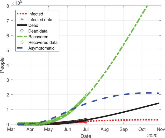
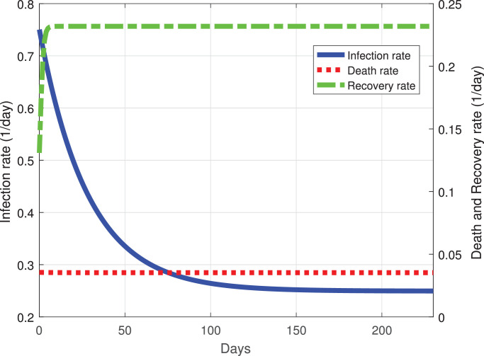
The predicted evolution of the outbreak for COVID-19 in Mexico can be seen in Fig. 2 . The parameters of the mathematical model were fitted with the experimental data provided by a daily update from the Mexican Ministry of Health. By adjusting the data from the period from March 12, 2020 to July 2, 2020, we simulated the daily new COVID-19 cases in Mexico until November 2020. Fig. 3 shows the variation of the infection rate β(t), recovery rate γ(t) and death rate δ(t) with respect to time. The infection rate decreases at a good pace with respect to time, taking roughly 70 days from March 12 to an infection rate per day of 0.3. At 200 days past March 12, the infection rate will be between 0.25 and 0.2, this means that in Mexico, there will be new cases of COVID-19 developing in a new normality of living with the virus. The recovery rate in Mexico at ten days past March 12 is increasing, and past the 10th day the recovery rate becomes constant with respect to time. This type of behavior may be explained by the fact that, at first, there were only mild cases in Mexico. Then, by March 22 there were much more severe cases, which are associated with a death rate that remains roughly constant at a rate of 0.04 per day.

Fig. 2.

Graphs for the spread of COVID-19 in Mexico. The dotted red line represents infected individuals, the solid black line represents the fatalities by the disease, the dash-dot green line represents recovered individuals, finally, the dashed blue line represents infected individuals but without any type of symptoms. (For interpretation of the references to color in this figure legend, the reader is referred to the web version of this article.)

Fig. 3.

Best fit values of the infection, recovery and death rates as functions of time. Dotted red line is the death rate, dash-dot green line the recovery rate and the solid blue line the infection rate. (For interpretation of the references to color in this figure legend, the reader is referred to the web version of this article.)

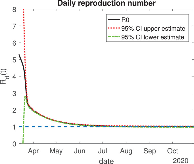
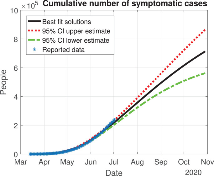
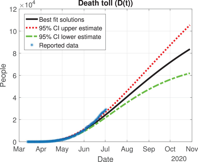
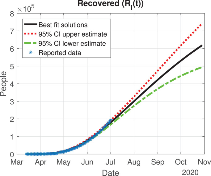
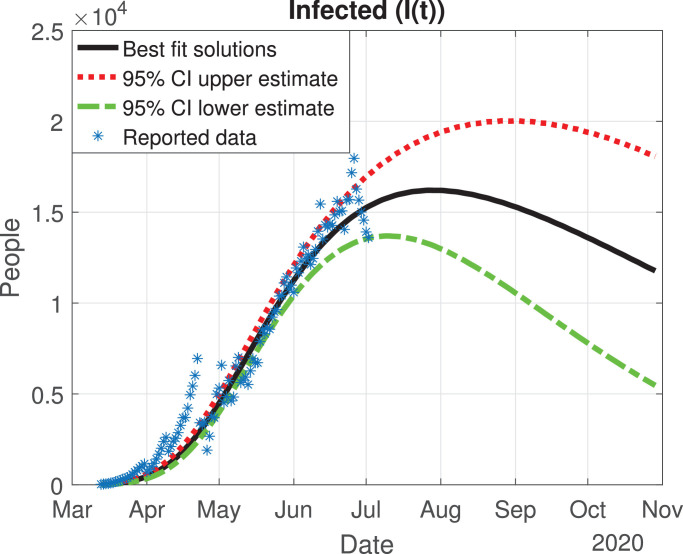
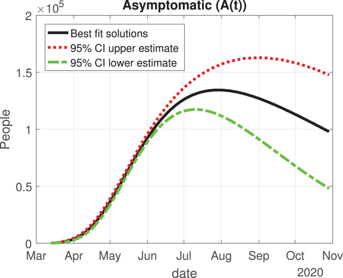
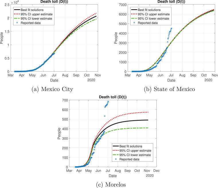
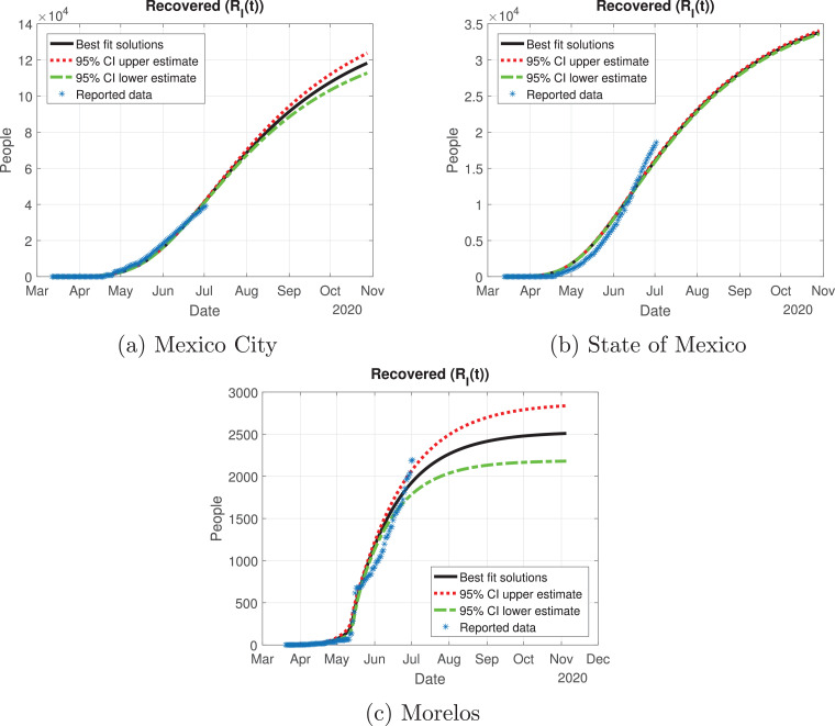
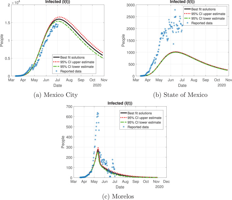
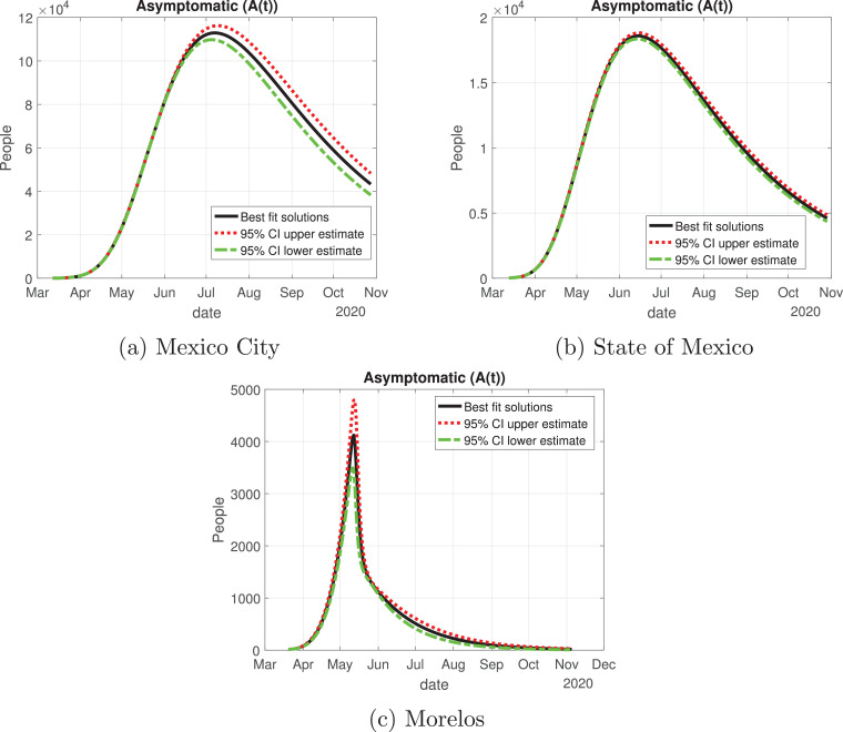
The values of the best fit parameters are given in Table 1 . We also include there the lower and upper bounds of the 95% confidence intervals obtained after the MCMC approach. Using these values for the parameters, we can calculate the effective daily reproduction ratio R_d(t) for each day (see Fig. 4 ). As we can see in Fig. 4, during March R_d(t) decreases exponentially to a value of 2, although there is a large uncertainty about its exact value in the first days, then it decreases from 2 to 1 during the months of April, May and June. The decrease from the first period is very helpful and Mexico will be entering a declared phase two of the pandemic with a relatively low reproduction number. We believe this decay may have occurred because the Ministry of Health applied the “Jornada Nacional de Sana Distancia” before Mexico declared to be in phase two. Our simulation shows that R_d(t) will become 1 by the month of July, and it will maintain this value until past October 2020. In Fig. 5, Fig. 6, Fig. 7, Fig. 8, Fig. 9 , we carried out the simulation with the best fit parameters and confidence intervals. We show a comparison of the cumulative number of infections (Fig. 5), deaths (Fig. 6) and recovered cases (Fig. 7) with the reported data. We also plot the number of active symptomatic infections and asymptomatic infections in Figs. 8 and 9, respectively. Our simulations show that the peak of the infection will most likely occur between July and September 2020.

Table 1.

Model parameters obtained from the best fit optimization for Mexico.

Parameter	Best fit value for Mexico	95% CI	Unit
β0	0.4646	(0.4192, 0.5100)	1/day
β1	0.2514	(0.2403, 0.2625)	1/day
τβ	29.0893	(27.2078, 30.9709)	day
γ0	0.0895	(0.0222, 0.1567)	1/day
γ1	0.1539	(0.0937, 0.2140)	1/day
τγ	7.7042	(5.4516, 9.9568)	day
δ0	0.0097	(0.0051, 0.0144)	1/day
δ1	0.0355	(0.0329, 0.0381)	1/day
τδ	6.4256	(4.6097, 8.2415)	day
w	0.2805	(0.2676, 0.2934)	1/day
p	0.1185	(0.1112, 0.1258)	–

Fig. 4.

Variation of the effective daily reproduction number through time. The solid black line represents the value of the reproduction number; the red dotted and green dash-dot lines are the 95% confidence interval upper and lower bounds, respectively. The blue dashed line represents the value one. (For interpretation of the references to color in this figure legend, the reader is referred to the web version of this article.)

Fig. 5.

Cumulative number of symptomatic infected individuals ($I\left(t\right)+R_I\left(t\right)+D\left(t\right)$) predicted by the model, 95% confidence interval and reported cases.

Fig. 6.

Death toll (D(t)) predicted by the model, 95% confidence interval and reported number of fatalities.

Fig. 7.

Number of recovered cases (R_I(t)) predicted by the model, 95% confidence interval and reported number of recoveries.

Fig. 8.

Number of infected cases (I(t)) predicted by the model, 95% confidence interval and number of active infections computed from the reported data.

Fig. 9.

Number of asymptomatic cases (A(t)) predicted by the model and 95% confidence interval.

4.2. Heterogeneity of the outbreak of COVID-19 in two regions in Mexico

We evaluated the heterogeneity of the spread of COVID-19 in Mexico. We applied our SEIARD model for two important regions in Mexico: the Mexico Valley (Mexico City, State of Mexico and Morelos) and the Yucatan Peninsula (Campeche, Quintana Roo and Yucatan).

4.2.1. Mexico Valley

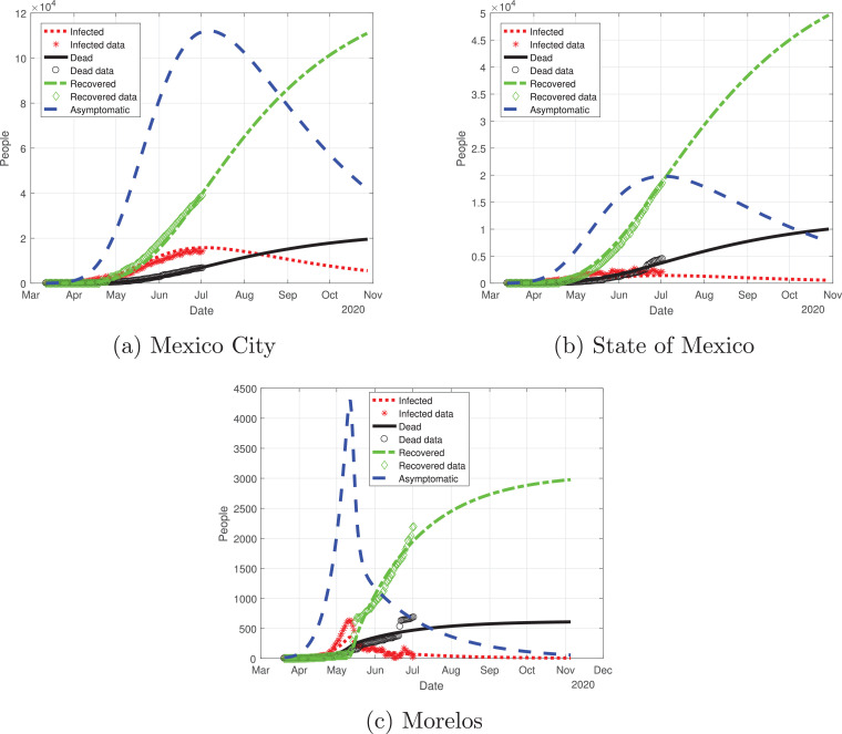
First, we modeled the evolution of the outbreak of COVID-19 in the Valley of Mexico, which is shown in Fig. 10 . We adjusted the data provided by the Mexican Ministry of Health from March 12 to July 2 and simulated the daily cumulative cases for each state until November 2020. The outbreak in the Mexico Valley will be slightly different from the national perspective, and each state will behave differently.

Fig. 10.

Graphs for the spread of COVID-19 in the Valley of Mexico. Dotted red lines represent infected individuals, solid black lines represent the fatalities by the disease, dash-dot green lines represent recovered individuals, finally, dashed blue lines represent infected individuals but without any type of symptoms. (For interpretation of the references to color in this figure legend, the reader is referred to the web version of this article.)

Mexico City outbreak is different from the other states, even though it had the largest number of infections: the curve for the infected population there (red line in Fig. 10a) increased in a controlled way, reaching its peak in early July and starting to descend from July to November. State of Mexico (Fig. 10b) has the same behavior as Mexico City, the only difference is the number of infected individuals. Morelos (Fig. 10c) had a different cycle of the pandemic: the infected individuals increased exponentially by early May, reaching its peak in mid-May; then, the number of infected individuals decays at a good pace from June to November. The difference in the peak may be due to the separation of the capital of Morelos from Mexico City (86.6 km). Also, the connection between these states was cut off due to the confinement declared by the Ministry, which may be a reason for the difference between the outbreak of the infection in these states.

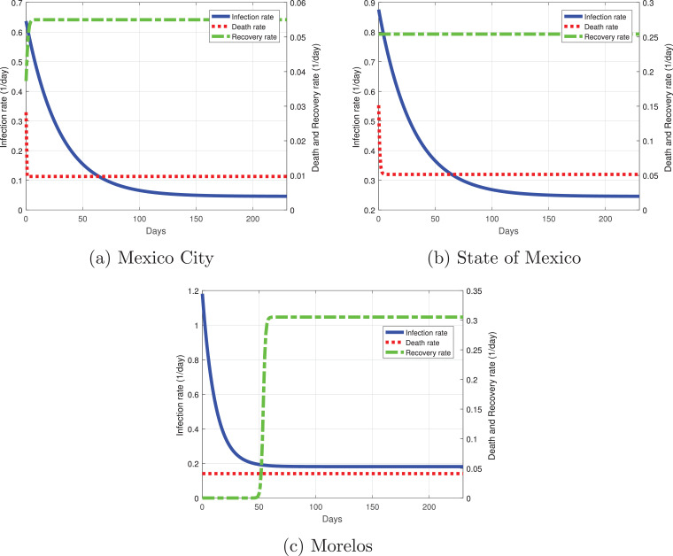
Fig. 11 shows the variation of the infection, recovery rate and death rate for the Mexico Valley. The rates between these states are different: Mexico City (the capital of Mexico, which has one of the two more important airports of the country) has the lowest infection rate in the initial days of the simulation, being only a little above 0.6. At 60 days past March 12, the infection rate becomes roughly 0.1 and decays as time passes. The recovery rate in Mexico City starts with severe cases at the early days of the outbreak, and it will eventually remain constant, having not only severe cases but mild ones as well. The death rate at the initial days of the outbreak was 0.03, which is associated with only having severe cases during the early days, but then the death rate decayed and remained constant with a value of 0.01. The infection rate in the State of Mexico is higher than in Mexico City being around 0.9, but it decays rapidly as time passes with a value of 0.3 at 60 days past March 12; the State of Mexico will have a similar behavior for the infection rate as the national perspective: it will be around 0.25 at 200 days past March 12. The recovery rate remains constant throughout the outbreak, by having at first severe cases, then developing mild cases as well. There has been data indicating that most of the severe cases from the State of Mexico were treated by the hospitals in Mexico City. The death rate has the same behavior as in Mexico City, the only difference is that at early days many patients died at a rate of 0.15. Morelos was the state with a higher infection rate from the Mexico Valley with a value of 1.2, which can be seen in Fig. 10c as the infected population increased exponentially, but it decayed rapidly to 0.2 at 30 days past March 12 and has remained constant since then. The recovery rate at first was very low, this means that there were severe cases at the initial days of the outbreak; at 50 days past March 12, the recovery rate increased due to the presence of milder cases. The death rate for Morelos remained constant at a value of 0.05.

Fig. 11.

Best fit parameters of the infection, death and recovery rates as functions of time for the Valley of Mexico. Dotted red line is the death rate, dash-dot green line the recovery rate and the solid blue line the infection rate. (For interpretation of the references to color in this figure legend, the reader is referred to the web version of this article.)

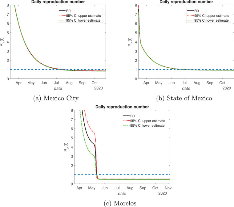
The daily reproduction ratio for Mexico City (Fig. 12 a) behaved differently than the other states. At first, it had a value higher than 8; from May to July, the value decayed exponentially until becoming equal to 1. By August the value will be lower than one, but we believe this city should be treated differently to the other states in the Mexico Valley since Mexico City has a much higher influence of transients daily. This is due to citizens from the surrounding areas coming to this city to work, creating a larger population that comprises not only people living in Mexico City, but citizens from the State of Mexico and Morelos as well. The State of Mexico has the same behavior for the daily reproduction ratio as Mexico City. The behavior for Morelos is by far different: in the month of April its value was higher than 8, which was associated with an increase of the infected population, and by mid-May, its value decayed rapidly to be lower than one, and it has been the same value since. The lockdown measures in this state were strengthened when the infected cases increased rapidly, and those actions are viewed in the daily reproduction ratio.

Fig. 12.

Variation of the effective daily reproduction number through time for the Mexico Valley. The solid black line represents the value of the reproduction number; the red dotted and green dash-dot lines are the 95% confidence interval upper and lower bounds, respectively. The blue dashed line represents the value one. (For interpretation of the references to color in this figure legend, the reader is referred to the web version of this article.)

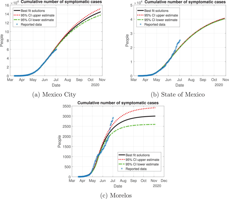
In Fig. 13, Fig. 14, Fig. 15, Fig. 16, Fig. 17 , we carried out the simulation with the best fit parameters and confidence intervals. We show a comparison of the cumulative number of infections: as we can see, Mexico City (Fig. 13a) will have the greatest number of infections within the pandemic of COVID-19, the State of Mexico (Fig. 13b) will be the second state with most infections. Mexico City will have most of the fatalities caused by the virus, followed by the State of Mexico, which has the cities with higher population than the rest of the states (Fig. 14) with the reported data. We also plot the number of recovered cases in Fig. 15 and the number of active symptomatic infections and asymptomatic infections in Figs. 16 and 17, respectively. Asymptomatic individuals are of great importance as they present a much higher number with respect to symptomatic individuals, by activating the “Jornada Nacional de Sana Distancia”, the number of symptomatic infections has been reduced and the curve of these individuals has been flattened as well.

Fig. 13.

Cumulative number of symptomatic infected individuals $C\left(t\right)=I\left(t\right)+R_I\left(t\right)+D\left(t\right)$ predicted by the model, 95% confidence intervals and reported cases for the Mexico Valley.

Fig. 14.

Death toll (D(t)) predicted by the model, 95% confidence intervals and reported number of fatalities for the Mexico Valley.

Fig. 15.

Number of recovered cases (R_I(t)) predicted by the model of the Mexico Valley, 95% confidence intervals and reported number of recoveries.

Fig. 16.

Number of infected cases (I(t)) predicted by the model of the Mexico Valley, 95% confidence intervals and number of active infections computed from the reported data.

Fig. 17.

Number of asymptomatic cases (A(t)) predicted by our model for the Mexico Valley and 95% confidence intervals.

4.2.2. Yucatan Peninsula

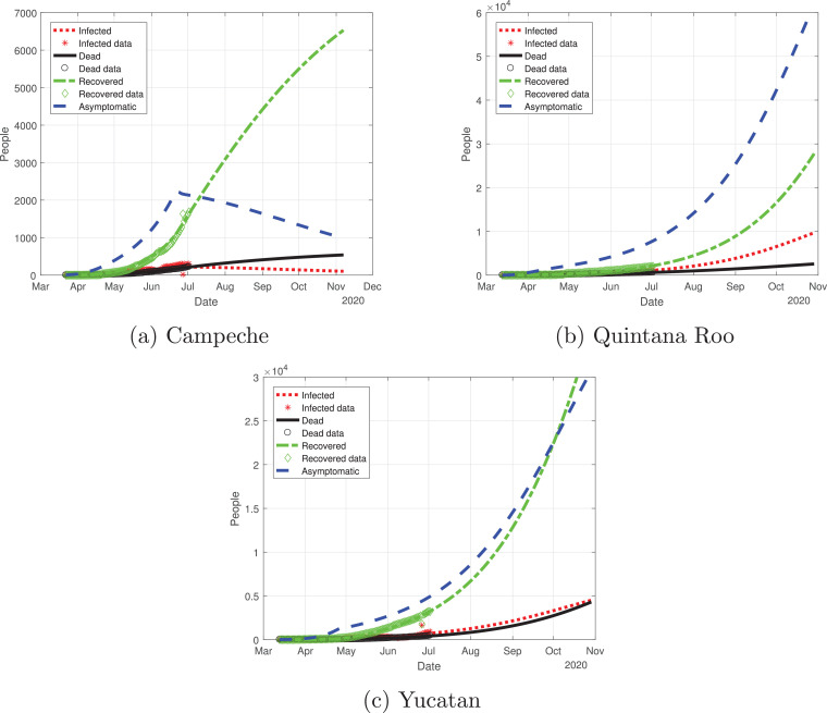
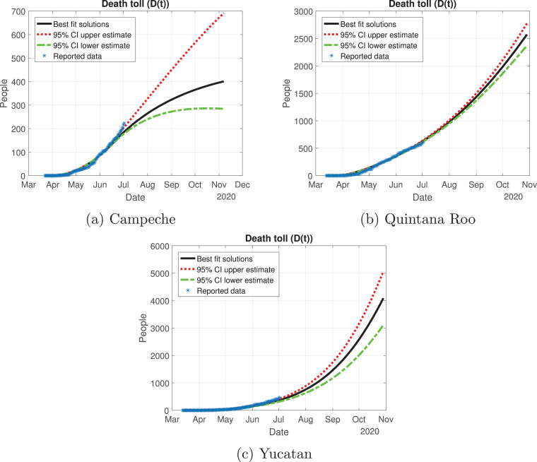
Now, we evaluate the outbreak in the Yucatan Peninsula. We reviewed Campeche, Yucatan and Quintana Roo; the outbreaks are depicted in Fig. 18 . Campeche is the only state that has reached a peak, and it was around mid-June. For the states of Yucatan and Quintana Roo, the cases are still increasing, which means that the cycle in these regions is far from over.

Fig. 18.

Graphs for the spread of COVID-19 in the Yucatan Peninsula. Dotted red lines represent infected individuals, solid black lines represent the fatalities by the disease, dash-dot green lines represent recovered individuals, finally, dashed blue lines represent infected individuals but without any type of symptoms. (For interpretation of the references to color in this figure legend, the reader is referred to the web version of this article.)

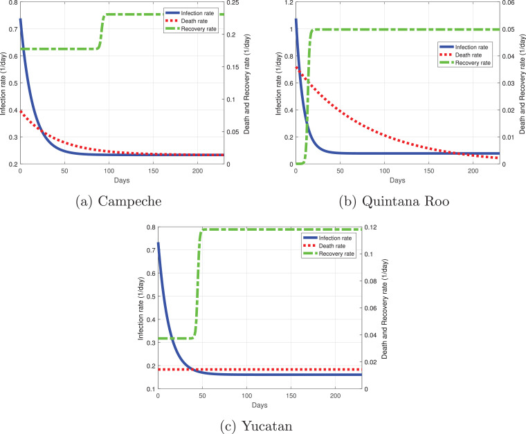
Campeche has a similar infection rate as Yucatan with a value of 0.72 at the initial stage of the outbreak (Fig. 19 a). It decayed rapidly by day 50 of the outbreak, when it has a rate of 0.25 and then remains constant. Its recovery rate was the highest from the Yucatan Peninsula, at first a lot of severe cases developed and few mild cases; 100 days must pass for its recovery rate could increase. When we wrote this manuscript, Campeche was a state of great concern because it had a death rate much higher than the rest of the states in the Yucatan Peninsula, its death rate started around 0.1 per day, but as time passed, the death rate decayed, becoming lower than 0.05. Quintana Roo has the highest infection rate of the Peninsula with a value equal to 1.1 at the beginning of the simulation (Fig. 19b), but it decays rapidly around 30 days from March 12; the infection rate will be around 0.1 by May 2020. The recovery rate for Quintana Roo starts very low with severe cases, and as days pass, the recovery rate increases with in theory a higher number of mild cases. The death rate at the initial days was higher in Quintana Roo with a value of 0.035;as the days pass, the rate decreases, indicating that severe and mild cases are recovering more often. Finally, in the state of Yucatan, the infection rate started around 0.71; at 50 days past March 12, it remains constant at a value slightly lower than 0.2. The recovery rate for Yucatan has a similar behavior to the rest of the states but with different dynamics. At first, there were a lot of severe cases where the recovery may last longer; 40 days later, the recovery rate began to increase, which meant that more individuals recovered from COVID-19. Lastly, the death rate for Yucatan remained constant with a value lower than 0.02.

Fig. 19.

Best fit parameters of the infection, death and recovery rates as functions of time for the Yucatan Peninsula. Dotted red line is the death rate, dash-dot green line the recovery rate and the solid blue line the infection rate. (For interpretation of the references to color in this figure legend, the reader is referred to the web version of this article.)

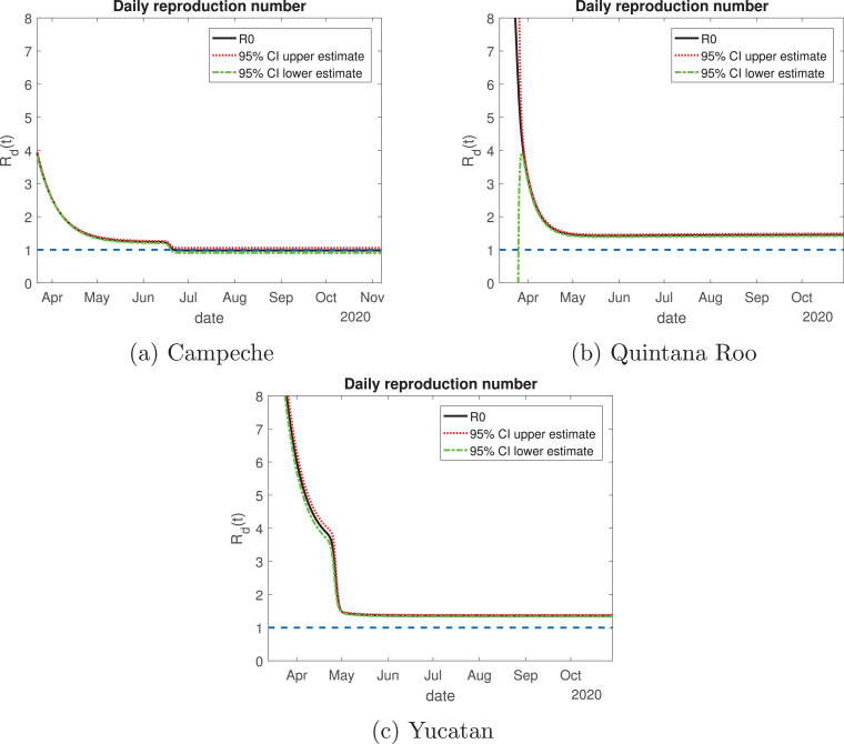
Regarding the daily reproduction ratio, Campeche is the state whose value is the smallest from the Yucatan Peninsula: it started with a value of 4 (Fig. 20 a), they will enter Phase 2 with a value smaller than 2. From the last week of June to November, its value will be around one, which means that the disease is decaying in the number of new infections with respect to the previous months. For the state of Quintana Roo (Fig. 20b), it started with a very high value but descended rapidly by mid-April, becoming less than 2. By June, the daily reproduction ratio remains constant with a value between 1 and 2, this means that the disease is increasing at a very low rate. Yucatan has a similar behavior as Quintana Roo (Fig. 20c), starting with a value greater than 8; by the month of May the value of the R_d(t) decayed exponentially to a value between one and 2, then it remains constant throughout the outbreak.

Fig. 20.

Variation of the effective daily reproduction number throughout time for the Yucatan Peninsula. The solid black line represents the value of the reproduction number; the red dotted and green dash-dot lines are the 95% confidence interval upper and lower bounds, respectively. The blue dashed line represents the value one. (For interpretation of the references to color in this figure legend, the reader is referred to the web version of this article.)

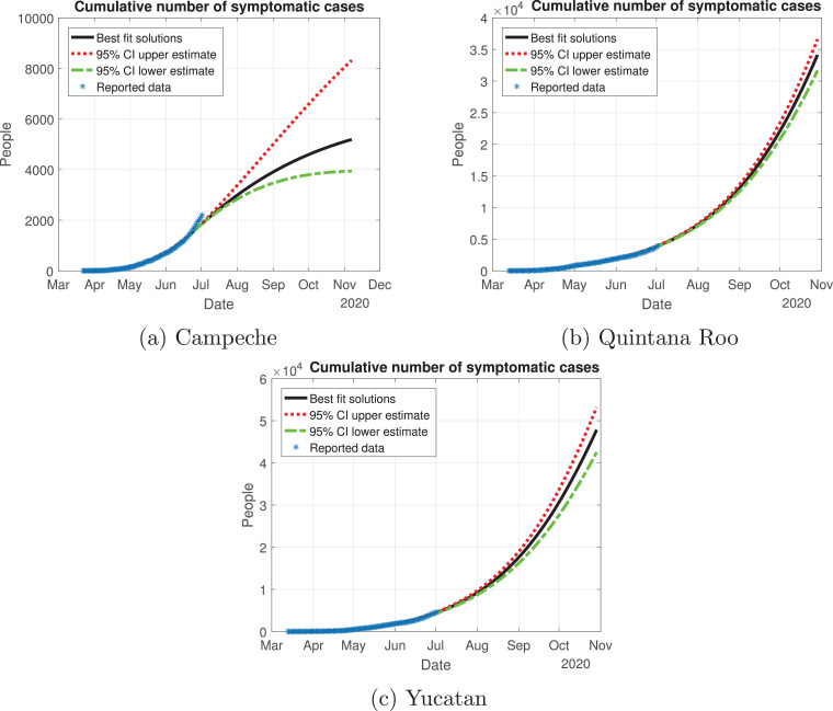
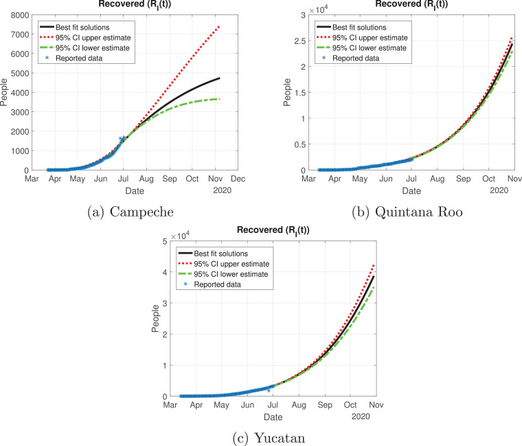
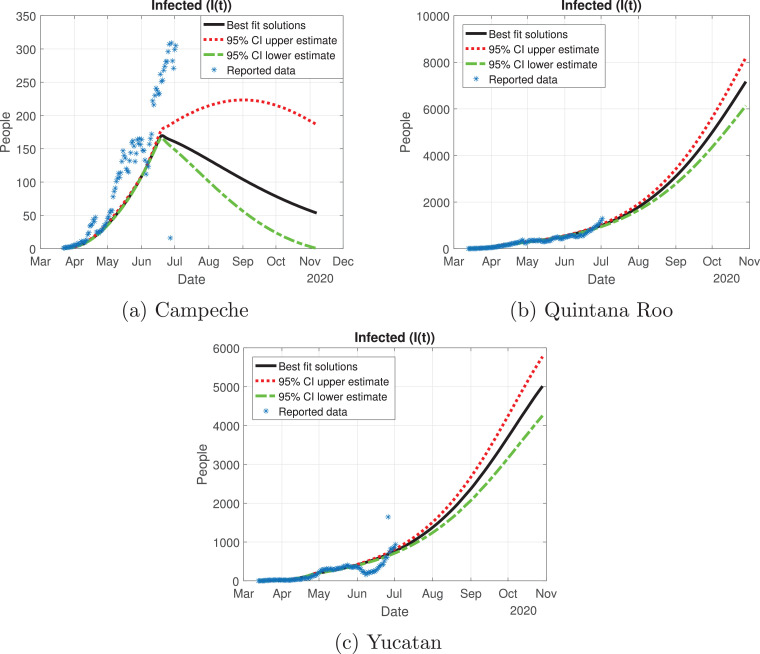
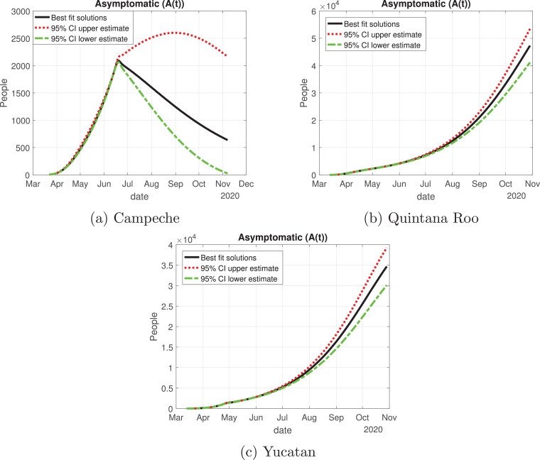
Quintana Roo and Yucatan are states of great importance for this Peninsula, because the cycle of the pandemic is still active, and it is slightly increasing since the month of June. We thought Quintana Roo (Fig. 21 b) was going to have a higher number of infected individuals, but Yucatan will have much more than the other states (Fig. 21c). Importantly, the cumulative number of symptomatic cases in these states is still increasing and thus is not showing any type of descend. Campeche will have between 4000 and 9000 infected individuals (Fig. 21a). The death toll will be higher in Yucatan (Fig. 22 c), and then Quintana Roo (Fig. 22b). We also plot the number of recovered cases in Fig. 23 and the number of active symptomatic infections in Fig. 24 . Finally, we can see in Fig. 25 the simulation of the asymptomatic cases, which shows that in the Yucatan Peninsula the cycle of the pandemic is far from over.

Fig. 21.

Cumulative number of symptomatic infected individuals $C\left(t\right)=I\left(t\right)+R_I\left(t\right)+D\left(t\right)$ predicted by the model, 95% confidence intervals and reported cases for the Yucatan Peninsula.

Fig. 22.

Death toll (D(t)) predicted by the model, 95% confidence intervals and reported number of fatalities for the Yucatan Peninsula.

Fig. 23.

Number of recovered cases (R_I(t)) predicted by the model of the Yucatan Peninsula, 95% confidence intervals and reported number of recoveries.

Fig. 24.

Number of infected cases (I(t)) predicted by the model of the Yucatan Peninsula, 95% confidence intervals and number of active infections computed from the reported data.

Fig. 25.

Number of asymptomatic cases (A(t)) predicted by our model for the Yucatan Peninsula and 95% confidence intervals.

5. Discussion

During the outbreak of a pandemic where the transmission is from infected individuals to healthy individuals, the use of mathematical models as a forecast is of great importance. By this approach, authorities can plan a health care program and control the spread even with limited resources. In this work, we formulated and analyzed a compartmental mathematic epidemic model to simulate the outbreak of the virus in mainland Mexico and important regions of said country.

Our mathematical model was a data driven analysis, using publicly available data from our Ministry of Health, which are updated daily. Our model incorporates two compartments that are of the utmost importance: exposed and asymptomatic. By incorporating the exposed subpopulation, we are modeling the latency period, and the asymptomatic subpopulation incorporates the individuals that do not present any type of symptoms but have the ability to spread the virus and infect more individuals. Both tools are important to understand the size and time of the outbreak.

The results of our numerical solutions would let us compare how different the outbreak will be in the two studied regions. For overall Mexico, we used the cumulative infections for all 32 states. The Valley of Mexico will be the region with most infected individuals and deaths, because this region concentrates 22% of the Mexican population. Nevertheless, there is still heterogeneity in the Valley of Mexico: Mexico City and the State of Mexico present a similar behavior, but in Mexico City they will be more infected individuals with or without symptoms. Even though control measures like social distancing were applied and the curve of infected individuals is flattened, there will be a high number of infected individuals with symptoms. This being said, Mexico should focus their effort in applying hospital interconnection and have sufficient resources to help all individuals who will develop severe respiratory symptoms.

On June 1, the “Jornada Nacional de Sana Distancia" came to an end, by this day Mexico entered in a new normality governed by a system very similar to a traffic light system. The traffic light color is determined following 4 criteria:

• •Hospital occupation.
• •Evolution of the daily effective number R_t.
• •The tendency of the hospitalized cases.
• •The shift of the suspected cases.

Based on these criteria, the economic reactivation was determined with the epidemic risk with 4 colors (red, orange, yellow and green), the federal government established the measures that each state should implement in the midst of the pandemic. This strategy is focused on releasing the optimal number of individuals from quarantine, without jeopardizing the hospital occupation. As we can see, the effective daily reproduction ratio for the Valley of Mexico is below one for the three states evaluated, which means that these states are implementing the measures to try to prevent the spread of the virus in this new normality. It is important to mention that the Mexico Valley entered in orange traffic light in the last week of June, by the time we modeled our data we didn’t see any increase in the number of active cases.

For the Yucatan Peninsula, Quintana Roo and Yucatan have a very different behavior from Campeche. Regarding the effective reproduction number, Campeche is the only state that reaches a value below or equal to one, hence the disease is decreasing in that state. Yucatan and Quintana Roo are states where Mexico should focus their actions in supplying medical stock, because these regions are having an increase in the number of infected individuals. Yucatan has an alarming behavior, during the “Jornada Nacional de Sana Distancia”, the number of active cases (hospitalized or isolated in their houses) increased in the two weeks following the reopening of non-essential activities. We recommend that Yucatan and Quintana Roo go back to the red color of the traffic light system, because the health measures implemented were not enough and it is possible that a saturation of the hospital capacity to treat severe COVID-19 cases occurs.

CRediT authorship contribution statement

Ugo Avila-Ponce de León: Conceptualization, Methodology, Software, Formal analysis, Data curation, Writing - original draft, Writing - review & editing. Ángel G.C. Pérez: Conceptualization, Methodology, Software, Formal analysis, Writing - review & editing. Eric Avila-Vales: Conceptualization, Methodology, Supervision, Project administration.

Declaration of Competing Interest

The authors declare that they have no known competing financial interests or personal relationships that could have appeared to influence the work reported in this paper.

References

- 1.Zhang G., Zhang J., Wang B., Zhu X., Wang Q., Qiu S. Analysis of clinical characteristics and laboratory findings of 95 cases of 2019 novel coronavirus pneumonia in Wuhan, China: a retrospective analysis. Respir Res. 2020;21(1):1–10. doi: 10.1186/s12931-020-01338-8. [DOI] [PMC free article] [PubMed] [Google Scholar]
- 2.Coronaviridae Study Group of the International Committee on Taxonomy of Viruses The species severe acute respiratory syndrome-related coronavirus: classifying 2019-nCoV and naming it SARS-CoV-2. Nat Microbiol. 2020;5:536–544. doi: 10.1038/s41564-020-0695-z. [DOI] [PMC free article] [PubMed] [Google Scholar]
- 3.Urso D.L. Coronavirus disease 2019 (COVID-19): A brief report. Clin Manag Issues. 2020;14(1):15–19. [Google Scholar]
- 4.Cruz-Pacheco G., Bustamante-Castaneda F.J., Caputo J.G., Jimenez-Corona M.E., Ponce-de Leon S. Dispersion of a new coronavirus SARS-CoV-2 by airlines in 2020: Temporal estimates of the outbreak in Mexico. medRxiv2020. [DOI] [PubMed]
- 5.Alvarez M.M., Gonzalez-Gonzalez E., Trujillo-de Santiago G.. Modeling COVID-19 epidemics in an Excel spreadsheet: Democratizing the access to first-hand accurate predictions of epidemic outbreaks. medRxiv2020. [DOI] [PMC free article] [PubMed]
- 6.Acuña Zegarra M.A., Comas-García A., Hernández-Vargas E., Santana-Cibrian M., Velasco-Hernandez J.X. The SARS-CoV-2 epidemic outbreak: a review of plausible scenarios of containment and mitigation for Mexico. medRxiv2020.
- 7.Tang B., Wang X., Li Q., Bragazzi N.L., Tang S., Xiao Y., Wu J. Estimation of the transmission risk of the 2019-nCov and its implication for public health interventions. J Clin Med. 2020;9(2):462. doi: 10.3390/jcm9020462. [DOI] [PMC free article] [PubMed] [Google Scholar]
- 8.Lin Q., Zhao S., Gao D., Lou Y., Yang S., Musa S.S., Wang M.H., Cai Y., Wang W., Yang L., He D. A conceptual model for the coronavirus disease 2019 (COVID-19) outbreak in Wuhan, China with individual reaction and governmental action. Int J Infect Dis. 2020;93:211–216. doi: 10.1016/j.ijid.2020.02.058. [DOI] [PMC free article] [PubMed] [Google Scholar]
- 9.Zhao S., Chen H. Modeling the epidemic dynamics and control of COVID-19 outbreak in China. Quant Biol. 2020;8:11–19. doi: 10.1007/s40484-020-0199-0. [DOI] [PMC free article] [PubMed] [Google Scholar]
- 10.Khrapov P., Loginova A. Mathematical modelling of the dynamics of the Coronavirus COVID-19 epidemic development in China. Int J Open Inf Technol. 2020;8(4):13–16. [Google Scholar]
- 11.Fanelli D., Piazza F. Analysis and forecast of COVID-19 spreading in China, Italy and France. Chaos Solitons Fractals. 2020;134:109761. doi: 10.1016/j.chaos.2020.109761. [DOI] [PMC free article] [PubMed] [Google Scholar]
- 12.Caccavo D.. Chinese and Italian COVID-19 outbreaks can be correctly described by a modified SIRD model. medRxiv2020.
- 13.Annas S., Pratama M.I., Rifandi M., Sanusi W., Side S. Stability analysis and numerical simulation of SEIR model for pandemic COVID-19 spread in Indonesia. Chaos Solitons Fractals. 2020;139:110072. doi: 10.1016/j.chaos.2020.110072. [DOI] [PMC free article] [PubMed] [Google Scholar]
- 14.Cooper I., Mondal A., Antonopoulos C.G. A SIR model assumption for the spread of COVID-19 in different communities. Chaos Solitons Fractals. 2020;139:110057. doi: 10.1016/j.chaos.2020.110057. [DOI] [PMC free article] [PubMed] [Google Scholar]
- 15.Pai C., Bhaskar A., Rawoot V. Investigating the dynamics of COVID-19 pandemic in India under lockdown. Chaos Solitons Fractals. 2020;138:109988. doi: 10.1016/j.chaos.2020.109988. [DOI] [PMC free article] [PubMed] [Google Scholar]
- 16.Nadim S.S., Ghosh I., Chattopadhyay J.. Short-term predictions and prevention strategies for COVID-2019: A model based study. arXiv preprint arXiv:200308150 2020. [DOI] [PMC free article] [PubMed]
- 17.Rodrigues H.S., Monteiro M.T.T., Torres D.F.M. Conference papers in science. Vol. 2013. 2013. Sensitivity analysis in a dengue epidemiological model. [Google Scholar]; article ID 721406
- 18.Tang B., Bragazzi N.L., Li Q., Tang S., Xiao Y., Wu J. An updated estimation of the risk of transmission of the novel coronavirus (2019-nCoV) Infect Dis Model. 2020;5:248–255. doi: 10.1016/j.idm.2020.02.001. [DOI] [PMC free article] [PubMed] [Google Scholar]
- 19.COVID-19 Tablero México, http://datos.covid-19.conacyt.mx/index.php.
- 20.Zu J., Li M., Li Z., Shen M., Xiao Y., Ji F. SSRN. 2020. Epidemic trend and transmission risk of SARS-CoV-2 after government intervention in the mainland of China: a mathematical model study; p. 3539669. [Google Scholar]