

Abstract
While high-resolution proton density-weighted magnetic resonance imaging (MRI) of intracranial vessel walls is significant for a precise diagnosis of intracranial artery disease, its long acquisition time is a clinical burden. Compressed sensing MRI is a prospective technology with acceleration factors that could potentially reduce the scan time. However, high acceleration factors result in degraded image quality. Although recent advances in deep-learning-based image restoration algorithms can alleviate this problem, clinical image pairs used in deep learning training typically do not align pixel-wise. Therefore, in this study, two different deep-learning-based denoising algorithms—self-supervised learning and unsupervised learning—are proposed; these algorithms are applicable to clinical datasets that are not aligned pixel-wise. The two approaches are compared quantitatively and qualitatively. Both methods produced promising results in terms of image denoising and visual grading. While the image noise and signal-to-noise ratio of self-supervised learning were superior to those of unsupervised learning, unsupervised learning was preferable over self-supervised learning in terms of radiomic feature reproducibility.
Subject terms: Image processing, Translational research, Magnetic resonance imaging
Introduction
Compressed sensing in magnetic resonance imaging (MRI) is a commonly used signal processing technology for efficiently acquiring and reconstructing an MR signal. It is based on the principle that the sparsity of a signal can be exploited to recover it from significantly fewer samples than are required by the Shannon–Nyquist sampling theorem1,2. Along with sensitivity encoding using a receiver array (SENSE)3, compressed sensing technologies have also been introduced to reduce the MR scan time further4. Compressed SENSE (CS) that concurrently uses compressed sensing and sensitivity encoding has become the next generation MR technology, as it can significantly reduce the scan time of an MRI.
Among the MRI sequences commonly used for investigations on vessel wall, high-resolution proton density-weighted (HRPD) MRI of the intracranial vessel wall is significant, as it can provide excellent anatomic information on even tiny vascular structures based on high signal-to-noise ratios, thus providing precise diagnoses of intracranial artery disease and guidance in terms of the appropriate treatment decision5. Though there are other choices such as the T1 weighted image, PD is preferable as it can achieve a high signal-to-noise ratio6.
However, acquiring HRPD MR images takes a long time, particularly when using a spatial resolution of ≤ 0.4 mm3, which could cause patient discomfort and motion artefacts. To address this problem, CS can be applied to reduce the scan time while preserving image quality to some extent7,8. However, loss of image quality, as compared with a fully sampled MRI, is unavoidable. A previous study9 reported that CS HRPD MR images with high acceleration factors yields unacceptable imaging for radiological reading. As low-quality vessel wall imaging hampers accurate diagnosis9–11, improving the image quality of CS HRPD MR images would be beneficial for accurate radiological reading and diagnosis.
Furthermore, the significance of improving image quality is increasing for data-driven computer-based medical imaging research, as the information extracted from the images is impacted by noise12–14. Particularly in radiomics, which extracts quantitative features from medical images that may exhibit valuable medical information, reproducibility and generalisability is one of the biggest challenges13,14. Image quality difference among MRI images that are acquired using different imaging protocols is one of the factors the cause generalisability issues15,16. Therefore, improving image quality while preserving imaging features is essential in terms of image standardisation and generalisation.
Recently, image quality enhancement using a convolutional neural network (CNN) that aims to restore the corrupted, noisy images to clean images has achieved significant success in computer vision. In most cases, the image restoration networks were trained with corrupted–uncorrupted image pairs that are aligned pixel-wise and directly minimise the mean squared error (MSE) or absolute error between the input and output images of the network. However, this approach is not applicable for medical images in a routine clinical process, as it is difficult to collect real pixel-wise clean and unclean pairs of MR images owing to motion artefacts unless fully sampled k-space data is stored.
Similar issues also exist in low-dose computed tomography (CT) enhancement tasks. For instance, cardiac CT images at low- and high-dose phases have pixel misalignment problems due to cardiac motion. Therefore, respiratory motion artifacts may cause pixel-alignment problems between low-dose and high-dose CT images17,18.
To address this lack of training pairs in medical imaging, two deep-learning (DL)-based approaches offer the following possibilities: (1) pixel-wise training pairs can be obtained by artificially generating corrupted medical images19,20 or (2) unsupervised image translation networks can be applied based on generative adversarial networks (GAN)17,21.
In this study, we compared the network output images of two different DL-based approaches in terms of (1) quantitative and qualitative image quality enhancement and (2) imaging feature reproducibility for radiomics. In the first approach, we synthesised pixel-wise alignment training pairs by adding random Gaussian noise to clean MR images22. Thereafter, the network was trained for denoising the noisy high-acceleration CS HRPD MR images in the inference phase, as a self-supervised learning method. In the second approach, we utilised cycle-consistent adversarial networks17 to transfer noisy MR images to clean MR images, as an unsupervised learning method.
In summary, the main contributions of this paper are as follows:
We successfully reduced the noise in CS HRPD MR images using two different DL-based methods. Thereafter, denoising methods can further reduce the HRPD MR scan time with a lower compromise on image quality. Furthermore, the proposed methods are expected to be applied to other medical image restoration tasks without the pixel-wise alignment of training pairs.
This is the first study that directly compares two different DL-based image restoration methods. Therefore, we expect that this study will facilitate setting guidelines for choosing the appropriate image restoration network depending on the purpose.
Related works
Accelerating MRI acquisition is a topic that has gained significant attention in literature. Currently, parallel imaging hardware and compressed sensing MRI are frequently used in real clinical settings for fast MRI acquisition process. However, these reconstruction algorithms require multiple prior information. For instance, parallel MRI using coil sensitivity information and CS MRI reconstruction utilizes image sparsity as a prior for fast MRI reconstructions. With the recent advances in DL, several efforts have been made on fast MRI acquisition using DL-based methods. Compared with traditional methods, DL-based methods do not require enormous amounts of prior information. The DL-based method for fast MRI acquisition can be classified into four categories23: (1) Denoising acquired MRI images in the image domain24,25, (2) Updating both k-space domain and image domain using cascaded DL26–29, (3) Direct conversion of k-space data to image domain data through DL30, and (4) Interpolation of missing k-space data through DL and obtaining images through inverse Fourier transform23. Our study falls under category (1), which attempts to denoise the images in the post-processing steps. The direct use of the image domain, compared with k-space data, is advantageous, as it does not require additional information regarding k-space and coils. Furthermore, it has the potential to be used in other medical imaging devices other than MRI25.
Materials and methods
Image acquisition
The institutional review board for human investigations at Asan Medical Center (AMC) approved this study. Informed consent was obtained from all subjects. The research was performed in accordance with relevant guidelines and regulations. The study population and image acquisitions were as previously described9.
Study population
Fourteen healthy volunteers, including 7 men (mean age, 58.6 years; age range, 40–67 years) and 7 women (mean age, 55.3 years; age range, 33–65 years) with a general age of 56.6 years (age range, 33–67 years) were included in this study. All subjects underwent HRPD MRI for evaluation of intracranial arteries.
Image acquisition
A 3-T MRI system (Ingenia CX, Philips Medical System, Best, the Netherlands) with a 32-channel sensitivity-encoding head coil was used for all MR examinations. For delineation of the intracranial arteries, three-dimensional (3D) proton density-weighted imaging (PD) was carried out. CS HRPD MR images with a high acceleration factor (AFt 5.8) and original imaging sequence (SENSE PD with AFt 2.0) were acquired. The scan parameters are presented in Table 1. An example of the acquired dataset is displayed in Fig. 1.
Table 1.
Scan parameters of acquired proton density-weighted MR scans.
| CS AFt 5.8 | Original | |
|---|---|---|
| MRI acceleration technique | Compressed SENSE | SENSE |
| Scan duration | 4 min 22 s | 12 min 36 s |
| Extra-reduction factor | 2.9 | – |
| Acceleration factor (AFt) | 5.8 | 2.0 |
| Echo time (ms) | 35 | 35 |
| Repetition time (ms) | 2000 | 2000 |
| Flip angle (°) | 90 | 90 |
| Matrix | 300 × 300 × 75 | 300 × 300 × 75 |
| Field of view (FOV) (mm) | 120 × 120 × 30 | 120 × 120 × 30 |
| Voxel size (mm) | 0.4 × 0.4 × 0.4 | 0.4 × 0.4 × 0.4 |
| Sequence | 3D TSE | 3D TSE |
| Sampling Pattern | Radial-Cartesian | Radial-Cartesian |
| Reconstruction algorithm | Compressed sensing algorithm work in progress (Philips) | SENSE algorithm work in progress (Philips) |
Figure 1.
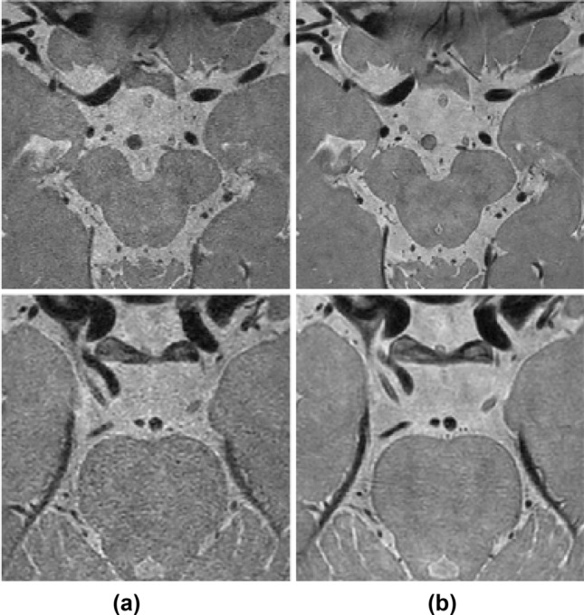
Example of dataset. Our dataset consists of (a) compressed SENSE (CS) AFt 5.8 and (b) original images (SENSE AFt 2.0).
General frameworks
Image denoising is a process that converts corrupted (noisy) input images into uncorrupted (clean) output images. This study aims to determine the mapping function for the transformation of a corrupted image into a clean image. Recently, deep convolutional neural networks (CNN) have performed well in determining the mapping function for image restoration31–33. Training the regression model of CNN is described as
where is loss function, is the corrupted input, is the uncorrupted target, and is the mapping function with the parameter .
In our dataset of noisy CS input images and clean original images, represents the noisy CS MR images and represents the clean original MR images. However, as there was a time interval during the acquisition of these images, the corresponding CS and original images do not have exact pixel-to-pixel alignment. Therefore, the loss function (typically L1 loss or L2 loss) could not represent the distance between the CS and original images in the manifold domain, as the pixel distance was inconsistent with the perceptual distance34. As presented in Fig. 2, the local structure of images acquired at the same position varied significantly between the acquired scans. As the local structure variations and other factors that resulted from the imaging acquisition process contributed significantly to the Euclidean pixel distance, the mean squared error and absolute error do not represent the differences in perceptual noise level. Therefore, we used two different DL-based image denoising methods to address this problem, as described in "Self-supervised learning" and "Unsupervised learning".
Figure 2.
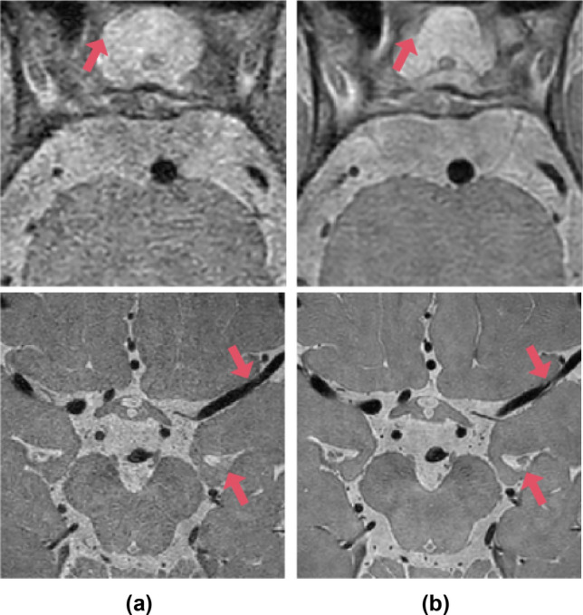
Local structure comparison between (a) CS AFt 5.8 and (b) original images (SENSE AFt 2.0). Details of local structure, such as cerebrospinal fluid (CSF) and blood vessels, vary between acquired magnetic resonance scans (red arrows).
Self-supervised learning
In self-supervised learning, we artificially generated corrupted input images , instead of directly using CS AFt 5.8 MR images as corrupted inputs, to preserve the pixel-wise alignment between the artificially generated input and target images. The corrupted MRI input images can be obtained in two different ways: (1) undersampling of k-space data or (2) corrupting the sampled data by adding noise. In both approaches, it is difficult to completely understand the noise distribution of the reconstructed MR images because of the black box nature of the acquisition process and its influence on the noise distribution35,36. In this study, we used the second approach for generating artificial inputs. The comparison between the two different noise modelling approaches is discussed in “Comparison of artificial noise modelling methods” section.
In general, it is well known that noise in the reconstructed MR image from a single coil follows Rician noise distribution37. Therefore, many MRI denoising studies are based on Rician noise distribution38–40. For instance38, successfully developed MRI Rician noise removal algorithm using spatially adaptive constrained dictionary learning. However, the nature of MRI noise became more complex as modern MR techniques, in particular, diverse parallel imaging techniques have been developed. The noise statistics of multi-coil parallel imaging MRI is still not fully understood and experimentally explored36. Therefore, we simply approximated the noise distribution as random Gaussian noise, as the noise distribution of multi-coil MR images can be approximated as random Gaussian noise22,41–44. Since we have obtained real corrupted CS AFt input images, we analysed noise distribution of CS 5.8 AFt images. The noise was measured in the air-filled anatomical region (e.g., a nasal cavity of size 10 × 10 matrices). A normality test was conducted based on D’Agostino and Pearson’s test45,46, using the SciPy normal test package. According to the results of the normality test, the noise distribution follows a normal distribution with P value > 0.01. Therefore, four our experiment, we approximated the noise model as a Gaussian noise model as follows :
| 1 |
where is the artificially generated corrupted input, is the clean target, and is Gaussian noise with mean and standard deviation .
The parameter was set to zero, with standard deviation ranges from 10 to 50% of the arithmetic mean. We selected the standard deviation range that gives the best network performance, i.e., the one which is 25–35% of the arithmetic mean. Figure 3 displays the target (original) and artificially generated input images. With the artificial corrupted images, the regression problem in the training phase can be written as follows:
| 2 |
where is the artificially generated corrupted input and is the clean target.
Figure 3.

Target original images (b, d) and artificial input images (a, c). Region of interest that contains basilar artery (left two columns) and middle cerebral artery (right two columns) inside red box are enlarged in lower column.
After training, inference is a simple feed-forward problem. In the inference phase, we replaced the artificial input with CS AFt 5.8 input images to dispose of noise in the real CS images (Fig. 4).
Figure 4.
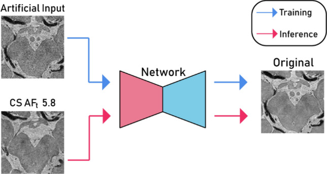
Basic implementation of self-supervised learning (encoder network, red; decoder network, cyan).
Recent deep CNN has employed encoder–decoder architecture for identifying the denoising algorithm. U-Net is a convolutional auto-encoder with skip connections47, which can capture high-level image details and reproduce it from corrupted images. Therefore, we utilised the basic structure of U-Net47 as a denoising network. A 2 × 2 max pooling layer was used for the down-sampling and a 2 × 2 transpose convolution layer was used for the up-sampling. In addition, w e added a batch normalisation layer before the activation layer and both the input and output channels were a single channel (Fig. 5).
Figure 5.

Denoising network architecture of U-Net used for self-supervised learning.
Unsupervised learning
In unsupervised learning, we implemented the cycle generative adversarial network (CycleGAN)17. The objective of CycleGAN is to map domain A to domain B and vice versa. With domain A as input images (CS AFt 5.8) and domain B as target images (original), the generators GAB, which maps A to B, and GBA, which maps B to A, are used with the discriminators DA, which discriminates real images from domain A and generated images, and DB, which discriminates real images from domain B and generated images (Fig. 6). The generators and discriminators were trained simultaneously. While pixel alignment was required in self-supervised learning, as the network was directly trained between input and target images using L1 loss, the loss functions of CycleGAN do not require pixel-to-pixel alignments. Therefore, pixel-misalignment problems can be eased with the unsupervised learning approach using CycleGAN. The optimisation problem is as follows17,48:
where
| 3 |
Figure 6.

Basic implementation of CycleGAN for unsupervised learning.
In further detail, the min–max problem of GAN loss with MSE can be represented as follows49:
| 4 |
Through the min–max optimisation, the generators attempt to learn the mapping functions of domain A to B (or B to A) that are sufficient enough to fool the discriminators, which attempt to classify the generated image from the real image to the best extent possible. The cyclic loss is defined as follows:
| 5 |
For the generator network, we utilised the same U-Net architecture (Fig. 5) as in self-supervised learning. Figure 7 depicts the architecture of the discriminator, which consists of five convolutional layers and a final fully connected layer. Each convolution layer, except the first convolution layer, is followed by an instance normalisation layer and a leaky ReLU layer; the instance normalisation layer is not included in the first layer. After the fully connected layer, the tensor was average-pooled and flattened into a 1 × 1 tensor.
Figure 7.

Discriminator architecture of unsupervised learning.
Training description
In self-supervised learning, the network was trained by minimising a loss function, which is the MSE between the input and output images. For training, we use input patches of size 256 × 256 from a noisy image with the corresponding clean patches. The number of epochs was 200 and the learning rate was set to 0.002. In the training phase, in which the denoising network is trained for artificial noise, 1,500 original MR images and artificial noise MR images were used for training and 300 images were used for validation. In the inference phase, which tests the performance of the denoising network, 300 CS AFt 5.8 MR images were used.
In unsupervised learning, MSE loss was used for GAN loss and L1 loss was used for cyclic loss. For training, we used input images of size 640 × 640. The number of epochs was 200 and the learning rate was set to 0.002. The same CS AFt 5.8 MR images and original images as described in the abovementioned self-supervised learning were used for training, validation, and testing.
Evaluation metric
The performance of the image denoising networks were evaluated both quantitatively and qualitatively. For the quantitative analysis, the image quality assessment could be divided into two major categories: (1) reference-based evaluation and (2) no-reference evaluation. In our study, reference-based evaluation metrics, such as MSE, peak signal-to-noise ratio, and structural similarity index, could not be applied, as our MR images did not have pixel-wise alignment reference images. Therefore, we evaluated the image quality of the network output images through no-reference evaluation metrics including signal-to-noise ratio (SNR), image noise, and Blind/Referenceless Image Spatial Quality Evaluator (BRISQUE) score. For the qualitative analysis, a neuroradiologist with more than 10 years of experience visually scored the network output MR images without the noise.
For the assessment of the statistical significance of the evaluation metrics, the Kolmogorov–Smirnov test was used to determine the normality of the distribution of the variables. Metrics for the comparison between input and output images, target and output images, and self-supervised and unsupervised output images were compared using paired t tests. Values of P < 0.05 were considered statistically significant. Statistical analyses were performed using the python SciPy stats package.
Image noise and signal-to-noise ratio
We measured image noise and SNR at the blood vessel wall of the middle cerebral, basilar, and internal carotid arteries. The intensity peaks at the blood vessel wall and decreases rapidly in the vessel lumen. Therefore, the signal was measured as the peak intensity in the blood vessel within a small region-of-interest (ROI) at the blood vessel wall, and the noise was obtained as the standard deviation of the vessel lumen (Eq. (6)):
| 6 |
While the intensity of the blood lumen was not uniform within the vessel lumen, we could compare the noise in the vessel lumen because we took the original image as reference. Furthermore, we measured the image noise and SNR at the cerebrospinal fluid (CSF) in the suprasellar cistern, interpeduncular cistern, and brain parenchyma (Eq. (7)).
| 7 |
Owing to inhomogeneous noise distribution caused by parallel imaging, noise cannot be simply measured in the air50,51. Instead, the signal and noise were measured as the mean and standard deviation of ROIs. The same ROIs of the vessel wall, CSF, and parenchyma were drawn for the CS AFt 5.8, original, and output images of the network.
BRISQUE
BRISQUE is a no-reference image quality assessment model that uses natural scene statistics in the spatial domain52. This model is composed of three steps: (1) extraction of natural scene statistics, (2) calculation of feature vectors, and (3) prediction of image quality score. We utilised a pretrained prediction model provided by Mittal et al.52 for predicting the image quality score. The minimum and maximum image scores are 0 and 100, respectively, with a lower image score indicating better image quality. The potential of BRISQUE as an indicator of medical image quality has been reported previously53 and it has been used to predict CS MRI reconstruction parameters54.
Radiomic feature extraction
For radiomic feature extraction, a large ROI of size 1,600 pixels in brain parenchyma was selected rather than vessel wall to avoid structural variation between the CS AFt 5.8 and original images. As the vessel wall is a small region surrounded by brain tissue, it could lead to variabilities in the radiomic features. As the purpose of the radiomics analysis is to investigate the effect of image quality enhancement on feature variations, the same ROI was drawn for the CS AFt 5.8, original, and output images of the network.
Thereafter, Lin’s concordance correlation coefficients (CCCs)55 were calculated between the input CS AFt 5.8 and original images, self-supervised output and original images, and supervised output and original images. A higher CCC score means higher reproducibility of radiologic features.
A total of 465 radiomics features were studied. The features include 18 first-order features, 75 texture features, and 380 wavelet features. The first-order features with intensity histograms include intensity range, energy, skewness, kurtosis, maximum, minimum, mean, uniformity, and variance. For texture analysis, the grey level co-occurrence matrix (GLCM), grey level run length matrix (GLRM), grey level size zone matrix (GLZM), neighbouring grey tone difference matrix (NGTDM), and grey level dependence matrix were calculated. For wavelet features, two-dimensional discrete wavelet transforms were performed in four directions: HH, HL, LH, LL, where ‘L’ indicates a low pass filter and ‘H’ refers to a high pass filter. We utilised open source software for radiomic feature analysis, Pyradiomics56.
Visual scoring
The HRPD MR images were assessed by a neuroradiologist with 10 years of experience, who was blinded to the sequence information. The images were rated for image quality and vessel delineation using a four-point visual scoring system (Table 2).
Table 2.
Visual scoring system used to evaluate image quality and vessel wall delineation.
| Score | Image quality and artifacts | Vessel delineation of outer contour and branching arteries |
|---|---|---|
| 3 | Excellent image quality without artifacts | Vessel is delineated with excellent signal and sharp contrast to the lumen and CSF |
| 2 | Good image quality with slight artifact | Vessel is delineated with adequate signal and contrast to lumen and CSF |
| 1 | Moderate image quality with moderate artifact | More than 50% of vessel is visible |
| 0 | Poor image quality with large artifact | Less than 50% of vessel is visible |
Results
Comparison of artificial noise modelling methods
The generation of corrupted input images in the k-space domain was common in studies related to fast MRI reconstruction24–27. Therefore, we followed the image quality enhancement methods, used on corrupted input images in the k-space domain, suggested by Wang et al.26. The method comprises the following steps:
The corrupted input images were obtained by undersampling the k-space domain using Poisson disk sampling mask, and then the images were reconstructed with zero-filling.
The super-resolution CNN network57 that maps the zero-filled MR images to the fully sampled clean images was trained.
The network output images were reconstructed through constrained CS-MR reconstruction optimization.
We followed the abovementioned steps, and then the method was applied to real noisy CS images. For the CS-MRI reconstruction method, we utilized a method suggested by Sparse MRI58, SigPy package. Compared with our self-supervised learning method, the noise and SNR measured in vessel wall, CSF, and parenchyma were significantly better in our self-supervised learning method (P < 0.01). The results of the comparison are shown in Fig. 8. While different noise modelling methods improved image quality, additive Gaussian noise was more effective in our dataset.
Figure 8.

Image noise and signal-to-noise ratio (SNR) results of input CS AFt 5.8 images, target original images, self-supervised learning output images, output images by Wang et al. at the blood vessel wall, CSF, and parenchyma. Paired t test results with **P < 0.01 and *P < 0.05.
Comparison of self-supervised learning and unsupervised learning approaches
The image noise, SNR of the vessel wall and CSF, BRISQUE scores, and radiomic feature reproducibility were measured in the input (CS AFt 5.8), target (original), and output images produced by the self-supervised and unsupervised learning approaches. The results of the denoising are displayed in Fig. 9.
Figure 9.

Image denoising results of (a) input, (b) target (original), and output images of (c) self-supervised and (d) unsupervised learning approaches. Middle cerebral and basilar arteries are enlarged in the second and fourth rows at a similar position.
Image noise and SNR measurement results
The image noise and SNR measurements are depicted in Fig. 10a–f. In both self-supervised and unsupervised learning, the image noise was decreased, and SNR was substantially increased compared with the input CS AFt 5.8 images (P < 0.05).
Figure 10.

Image noise (a, c, e), signal-to-noise ratio (SNR) (b, d, f), and BRISQUE (g) score results of input CS AFt 5.8 images (green), target original images (pink), self-supervised learning output images (purple), and unsupervised learning output images (yellow), at the blood vessel wall (a, b), CSF (c, d), and parenchyma (e, f). Paired t test results with **P < 0.01 and *P < 0.05.
When we compared the original images and the networks’ output images, the image noise of the self-supervised learning output images at the CSF and brain parenchyma was even lower than that of the original output images (P < 0.05). The SNR was also improved over that of the original images, except for in the CSF (P < 0.05). That is, the self-supervised learning output images had better image quality than the original images in terms of noise and the SNR.
None of the unsupervised learning output images were better than the original images (P > 0.05). In brain parenchyma, unsupervised learning output images were significantly inferior to the original images in terms of image noise and SNR (P < 0.01).
Furthermore, when we compared the SNR and noise at the vessel wall and brain parenchyma between the self-supervised and unsupervised learning output images, the SNR and noise were markedly better in the self-supervised learning output images (P < 0.05).
BRISQUE score results
The BRISQUE scores of the input (CS AFt 5.8), target (original), and output images of self-supervised and unsupervised learning are depicted in Fig. 10g. As described in Fig. 10, the BRISQUE scores of both self-supervised and unsupervised learning output images were lower than those of the input images (P < 0.01). That is, the output images were seen to be more natural owing to reduced noise52 compared with noisy input images. The difference between the original and unsupervised learning outputs was statistically meaningful (P < 0.01) and equal to approximately 1 point, whereas the difference between the input and target images was approximately 6 points.
Radiomic feature analysis
The CCCs between the input CS AFt 5.8 and original images, self-supervised output and original images, and unsupervised output and original images are presented in Table 3 and Fig. 11. After image quality enhancement, the CCCs between the output and original images were significantly improved for texture features and wavelet features in the unsupervised learning method (P < 0.01), whereas the changes were unknowable in the self-supervised learning method (P > 0.05).
Table 3.
Mean concordance correlation coefficient (CCCs) ± standard deviation between input CS AFt 5.8 and original images, unsupervised output and original images, and self-supervised output and original images. Paired t test results were indicated with **P < 0.01.
| Input CS AFt 5.8 vs original images | Supervised output vs original images |
Unsupervised output vs original images | |
|---|---|---|---|
| Texture features | 0.50 ± 0.28 | 0.47 ± 0.30 | 0.71 ± 0.20** |
| First-order features | 0.49 ± 0.28 | 0.43 ± 0.30 | 0.53 ± 0.35 |
| Wavelet features | 0.47 ± 0.28 | 0.47 ± 0.33 | 0.62 ± 0.28** |
Figure 11.

Concordance correlation coefficient (CCC) heat map of radiomics features. While CCCs between self-supervised learning output and original images remain relatively unchanged compared with those between input CS AFt 5.8 and output images, those between unsupervised output and original images improved notably.
Among 465 radiomics features, 86 features (18.5%) were reproducible in the input CS AFt 5.8 images and original images (based on a CCC > 0.859, including 17 out of 75 texture features, 3 out of 18 first-order features, and 66 out of 380 wavelet features (Fig. 12). For unsupervised learning output images, a total of 178 features (38.3%) were reproducible including 33 of 75 texture features, 6 out of 18 first-order features, and 139 out of 380 wavelet features. In the case of self-supervised learning output images, a total of 115 features (24.7%) were reproducible including 16 out of 75 texture features, 4 out of 18 first-order features, and 95 out of 380 wavelet features.
Figure 12.

Distribution of concordance correlation coefficient (CCC) between input and original images, unsupervised learning output and original images, and self-supervised learning output and original images.
Visual scoring on high-acceleration CS MR images by neuroradiologist
In terms of image quality, the mean visual scores were 1.00 for the input images, 1.92 for the output images (self-supervised images, 2.00; unsupervised images, 1.83), and 2.50 for the target images. The target images were significantly superior to the input and output images in terms of image quality, and the output images were also significantly superior to the input images in terms of image quality (P < 0.05). However, there were no significant differences in image quality between the self-supervised and unsupervised images (P > 0.05).
In the vessel delineation, the mean scores were 1.67 for the input images, 2.67 for the output images (self-supervised images, 2.67; unsupervised images, 2.67), and 3.00 for the target images. No significant differences were determined between the output (self-supervised and unsupervised) and target images (P > 0.05). The output (self-supervised and unsupervised) and target images were significantly superior to the input images (P < 0.05).
Discussion
In this paper, we presented two DL-based denoising methods for CS HRPD MR images with and without pixel-wise alignments. We demonstrated that both the methods achieved considerable performance in terms of image noise, SNR, BRISQUE scores, radiomic features, and visual scoring, as compared to the input CS AFt 5.8 images, which are not usable in routine clinical practice owing to low image quality60. The proposed methods may allow acquisition of more MR images per unit time and may also improve patient comfort. Furthermore, the reduced scan time will result in clearer MR images by avoiding motion artefacts that are commonly introduced by long image acquisition durations.
While both methods were promising in terms of image denoising without degradation of image texture, we found that the self-supervised learning outputs were superior in terms of SNR and image noise. In particular, the noise level of brain parenchyma output images obtained with self-supervised learning was even better than those of the target (original) images. This tendency was not observed for the output images of unsupervised learning. Figure 13 displays an example of the noise map, where noise was measured as the standard deviation in every 5 × 5 pixels. The noise pattern of the target image and unsupervised learning output images were similar, as generative adversarial networks learn the data distribution of the target images61.
Figure 13.

Noise map of original, self-supervised, and unsupervised learning output images. Area in red box in upper row was enlarged in bottom row.
In contrast, the noise within the brain parenchyma was significantly decreased in the output image of self-supervised learning. Two major factors are thought to affect the observed over-denoising in the output images of self-supervised learning: First, the noise distribution of the original MR images was not uniform62,63. As the self-supervised network was trained to learn the denoising of uniformly distributed noises, over-denoising could be observed in some regions. Second, the original MR images were not essentially noise-free images. In real clinical practice, noise-free fully sampled MR images is hard to be obtained, as MR data is known to be affected by multiple sources of noise, including thermal noise and electronic noise22,41. Therefore, the self-supervised network was indeed trained with noisy–noisy training pairs, rather than noisy–noise-free training pairs. The regression problem we wanted to solve (Eq. (2)) can be expressed as follows:
| 8 |
where and are the noisy input and noisy target, respectively. Although a true clean target was not observed, it is still possible to map the corrupted to the true clean target by solving the minimisation task (Eq. (8)) under the condition , which can be met when random noise was introduced to 32. As our original images contained random noise, it is not surprising that the self-supervised network outputs were indeed even more denoised than the target original images.
While the self-supervised learning method demonstrates a better result with respect to SNR and noise, the unsupervised learning method improved the reproducibility of radiomics features, whereas the self-supervised learning methods demonstrated no significant advantages in terms of radiomic feature reproducibility. For radiomics researches using multiple medical images with different image qualities, the unsupervised learning method would be advantageous in terms of standardisation and generalisation over the self-supervised learning method. In addition, generating artificial training pairs is not straightforward because of the complex nature of medical images. The unsupervised learning approach could ease this problem because it does not require noise modeling of complex medical images. Accordingly, appropriate DL algorithms should be chosen, depending on the purpose of image translation and the nature of the dataset.
The present study had several limitations. First, the dataset was limited to the CS HRPD MR images of the vessel walls. Further studies should include various image modalities and purposes. Second, our dataset only included the MR images of healthy volunteers. A future study should investigate whether the two different approaches are affected by the clinical diagnosis. Third, this study was limited owing to the small number of subjects as well as the use of a single-vendor MR scanner. In addition, the input CS AFt 5.8 images do not contain residual aliasing artifacts. For further studies, a larger number of subjects, including different types of patients, and various MR scanner types should be included.
Conclusion
In this paper, we presented and compared two DL-based denoising networks that are applicable to datasets with or without pixel-wise alignments. Both approaches demonstrated promising results when assessed quantitatively and qualitatively. While the self-supervised learning approach was superior to the unsupervised learning approach in terms of SNR and noise level, the unsupervised learning method demonstrated better radiomics feature reproducibility. This study forms the basis for other medical image translation tasks in which pixel-wise alignment is not available.
Acknowledgement
This work was supported by a grant from the Korea Health Technology R&D Project through the Korea Health Industry Development Institute (KHIDI), funded by the Ministry of Health & Welfare, Republic of Korea (HI18C0022, HI18C2383).
Abbreviations
- CNN
Convolutional neural network
- CS
Compressed SENSE
- CSF
Cerebrospinal fluid
- CT
Computed tomography
- DL
Deep learning
- GAN
Generative adversarial network
- HRPD
High-resolution proton density-weighted
- MR
Magnetic resonance
- MRI
Magnetic resonance imaging
- MSE
Mean squared error
- PD
Proton density-weighted imaging
- SENSE
Sensitivity encoding with receiver array
- SNR
Signal-to-noise ratio
Author contributions
All authors reviewed the manuscript. D.E.—manuscript writing, computational experiment and statistical analysis. R.J.—computational experiment. W.S.H.—clinical advice on data analysis. H.L.– conceptual feedback. S.C.J.—supervised study design, manuscript writing, database construction, data analysis, and project integrity. N.K.—supervised study design, manuscript writing, technical support and project integrity.
Data availability
Data sharing is not applicable to this article due to medical data privacy protect act.
Competing interests
The authors declare no competing interests.
Footnotes
Publisher's note
Springer Nature remains neutral with regard to jurisdictional claims in published maps and institutional affiliations.
These authors contributed equally: Seung Chai Jung and Namkug Kim.
Contributor Information
Seung Chai Jung, Email: dynamics79@gmail.com.
Namkug Kim, Email: namkugkim@gmail.com.
References
- 1.Donoho DL. For most large underdetermined systems of linear equations the minimal. J. Commun. Pure Appl. Math. J. Issued Courant Inst. Math. Sci. 2006;59:797–829. [Google Scholar]
- 2.Davenport, M. The fundamentals of compressive sensing. IEEE Signal Processing Society Online Tutorial Library (2013).
- 3.Pruessmann KP, Weiger M, Scheidegger MB, Boesiger P. SENSE: sensitivity encoding for fast MRI. Magn. Reson. Med. 1999;42:952–962. [PubMed] [Google Scholar]
- 4.Jaspan ON, Fleysher R, Lipton ML. Compressed sensing MRI: a review of the clinical literature. Br. J. Radiol. 2015;88:20150487. doi: 10.1259/bjr.20150487. [DOI] [PMC free article] [PubMed] [Google Scholar]
- 5.Lee SH, Jung SC, Kang DW, Kwon SU, Kim JS. Visualization of culprit perforators in anterolateral pontine infarction: high-resolution magnetic resonance imaging study. Eur. Neurol. 2017;78:229–233. doi: 10.1159/000479556. [DOI] [PubMed] [Google Scholar]
- 6.Mandell D, et al. Intracranial vessel wall MRI: principles and expert consensus recommendations of the American Society of Neuroradiology. Am. J. Neuroradiol. 2017;38:218–229. doi: 10.3174/ajnr.A4893. [DOI] [PMC free article] [PubMed] [Google Scholar]
- 7.Balu N, et al. Accelerated multi-contrast high isotropic resolution 3D intracranial vessel wall MRI using a tailored k-space undersampling and partially parallel reconstruction strategy. Magn. Reson. Mater. Phys., Biol. Med. 2019;32:343–357. doi: 10.1007/s10334-018-0730-8. [DOI] [PMC free article] [PubMed] [Google Scholar]
- 8.Zhu C, et al. Accelerated whole brain intracranial vessel wall imaging using black blood fast spin echo with compressed sensing (CS-SPACE) Magn. Reson. Mater. Phys., Biol. Med. 2018;31:457–467. doi: 10.1007/s10334-017-0667-3. [DOI] [PMC free article] [PubMed] [Google Scholar]
- 9.Suh CH, Jung SC, Lee HB, Cho SJ. High-resolution magnetic resonance imaging using compressed sensing for intracranial and extracranial arteries: comparison with conventional parallel imaging. Korean J. Radiol. 2019;20(3):487–497. doi: 10.3348/kjr.2018.0424. [DOI] [PMC free article] [PubMed] [Google Scholar]
- 10.Alexander MD, et al. High-resolution intracranial vessel wall imaging: imaging beyond the lumen. J. Neurol. Neurosurg. Psychiatry. 2016;87:589–597. doi: 10.1136/jnnp-2015-312020. [DOI] [PMC free article] [PubMed] [Google Scholar]
- 11.Mossa-Basha M, et al. Added value of vessel wall magnetic resonance imaging in the differentiation of moyamoya vasculopathies in a non-Asian cohort. Stroke. 2016;47:1782–1788. doi: 10.1161/STROKEAHA.116.013320. [DOI] [PMC free article] [PubMed] [Google Scholar]
- 12.Chaudhari AS, et al. Utility of deep learning super-resolution in the context of osteoarthritis MRI biomarkers. J. Magn. Reson. Imaging. 2019;51:768–779. doi: 10.1002/jmri.26872. [DOI] [PMC free article] [PubMed] [Google Scholar]
- 13.Rizzo S, et al. Radiomics: the facts and the challenges of image analysis. Eur. Radiol. Exp. 2018;2:36. doi: 10.1186/s41747-018-0068-z. [DOI] [PMC free article] [PubMed] [Google Scholar]
- 14.Park JE, Park SY, Kim HJ, Kim HS. Reproducibility and generalizability in radiomics modeling: possible strategies in radiologic and statistical perspectives. Korean J. Radiol. 2019;20:1124–1137. doi: 10.3348/kjr.2018.0070. [DOI] [PMC free article] [PubMed] [Google Scholar]
- 15.Yang F, Dogan N, Stoyanova R, Ford JC. Evaluation of radiomic texture feature error due to MRI acquisition and reconstruction: a simulation study utilizing ground truth. J Physica Medica. 2018;50:26–36. doi: 10.1016/j.ejmp.2018.05.017. [DOI] [PubMed] [Google Scholar]
- 16.Peerlings J, et al. Stability of radiomics features in apparent diffusion coefficient maps from a multi-centre test-retest trial. Sci. Rep. 2019;9:4800. doi: 10.1038/s41598-019-41344-5. [DOI] [PMC free article] [PubMed] [Google Scholar]
- 17.Kang E, Koo HJ, Yang DH, Seo JB, Ye JC. Cycle-consistent adversarial denoising network for multiphase coronary CT angiography. Med. Phys. 2019;46:550–562. doi: 10.1002/mp.13284. [DOI] [PubMed] [Google Scholar]
- 18.Boas FE, Fleischmann D. CT artifacts: causes and reduction techniques. Imaging Med. 2012;4:229–240. [Google Scholar]
- 19.Chen H, et al. Low-dose CT via convolutional neural network. Biomed. Opt. Express. 2017;8:679–694. doi: 10.1364/BOE.8.000679. [DOI] [PMC free article] [PubMed] [Google Scholar]
- 20.Geng, M. et al. Unsupervised/semi-supervised deep learning for low-dose CT enhancement (2018). arXiv:1808.02603
- 21.Armanious, K. et al. MedGAN: medical image translation using GANs (2018). arXiv:1806.06397. [DOI] [PubMed]
- 22.Aja-Fernández S, Vegas-Sánchez-Ferrero G, Tristán-Vega A. Noise estimation in parallel MRI: GRAPPA and SENSE. J. Magn. Reson. Imaging. 2014;32:281–290. doi: 10.1016/j.mri.2013.12.001. [DOI] [PubMed] [Google Scholar]
- 23.Han Y, Sunwoo L, Ye JC. k-space deep learning for accelerated MRI. IEEE Trans. Med. Imaging. 2019;39:377–386. doi: 10.1109/TMI.2019.2927101. [DOI] [PubMed] [Google Scholar]
- 24.Lee D, Yoo J, Tak S, Ye JC. Deep residual learning for accelerated MRI using magnitude and phase networks. IEEE Trans. Biomed. Eng. 2018;65:1985–1995. doi: 10.1109/TBME.2018.2821699. [DOI] [PubMed] [Google Scholar]
- 25.Han Y, et al. Deep learning with domain adaptation for accelerated projection-reconstruction MR. Magn. Reson. Med. 2018;80:1189–1205. doi: 10.1002/mrm.27106. [DOI] [PubMed] [Google Scholar]
- 26.Wang, S. et al. In 2016 IEEE 13th International Symposium on Biomedical Imaging (ISBI). 514–517 (IEEE).
- 27.Hammernik K, et al. Learning a variational network for reconstruction of accelerated MRI data. Magn. Reson. Med. 2018;79:3055–3071. doi: 10.1002/mrm.26977. [DOI] [PMC free article] [PubMed] [Google Scholar]
- 28.Wang S, et al. DeepcomplexMRI: exploiting deep residual network for fast parallel MR imaging with complex convolution. Magn. Reson. Imaging. 2020;68:136–147. doi: 10.1016/j.mri.2020.02.002. [DOI] [PubMed] [Google Scholar]
- 29.Wang, S. et al. DIMENSION: dynamic MR imaging with both k‐space and spatial prior knowledge obtained via multi‐supervised network training. NMR Biomed. e4131 (2019). [DOI] [PubMed]
- 30.Zhu B, Liu JZ, Cauley SF, Rosen BR, Rosen MS. Image reconstruction by domain-transform manifold learning. Nature. 2018;555:487–492. doi: 10.1038/nature25988. [DOI] [PubMed] [Google Scholar]
- 31.Lim, B., Sanghyun S., Heewon, K., Seungjun, N. & Kyoung, M.L. Enhanced deep residual networks for single image super-resolution. In Proceedings of the IEEE Conference on Computer Vision and Pattern Recognition Workshops, 136–144 (2017).
- 32.Lehtinen, J. et al. Noise2Noise: learning image restoration without clean data (2014). arXiv:1803.04189.
- 33.Mao, X.-J., Shen, C. & Yang, Y.-B. Image restoration using convolutional auto-encoders with symmetric skip connections (2016). arXiv:1606.08921.
- 34.Doersch, C. Tutorial on variational autoencoders (2016). arXiv:1606.05908.
- 35.St-Jean, S., De Luca, A., Tax, C. M., Viergever, M. A. & Leemans, A. Automated characterization of noise distributions in diffusion MRI data (2019). arXiv:1906.12121. [DOI] [PubMed]
- 36.Dietrich O, et al. Influence of multichannel combination, parallel imaging and other reconstruction techniques on MRI noise characteristics. Magn. Reson. Imaging. 2008;26:754–762. doi: 10.1016/j.mri.2008.02.001. [DOI] [PubMed] [Google Scholar]
- 37.Gudbjartsson H, Patz S. The Rician distribution of noisy MRI data. Magn. Reson. Med. 1995;34:910–914. doi: 10.1002/mrm.1910340618. [DOI] [PMC free article] [PubMed] [Google Scholar]
- 38.Wang, S. et al.2013 35th Annual International Conference of the IEEE Engineering in Medicine and Biology Society (EMBC). 4030–4033 (IEEE).
- 39.Basu, S., Thomas, F. & Ross, W. Rician noise removal in diffusion tensor MRI. In International Conference on Medical Image Computing and Computer-Assisted Intervention, 117–125, Springer, Berlin, Heidelberg (2006). [DOI] [PubMed]
- 40.Nowak RD. Wavelet-based Rician noise removal for magnetic resonance imaging. IEEE Trans. Image Process. 1999;8:1408–1419. doi: 10.1109/83.791966. [DOI] [PubMed] [Google Scholar]
- 41.Aja-Fernández, S. & Tristán-Vega, A. A review on statistical noise models for magnetic resonance imaging. LPI, ETSI Telecomunicacion, Universidad de Valladolid, Spain, Tech. Rep (2013).
- 42.Ding Y, Chung YC, Simonetti OP. A method to assess spatially variant noise in dynamic MR image series. Magn. Reson. Med. 2010;63:782–789. doi: 10.1002/mrm.22258. [DOI] [PubMed] [Google Scholar]
- 43.Koay CG, Özarslan E, Pierpaoli C. Probabilistic identification and estimation of noise (PIESNO): a self-consistent approach and its applications in MRI. J. Magn. Reson. 2009;199:94–103. doi: 10.1016/j.jmr.2009.03.005. [DOI] [PMC free article] [PubMed] [Google Scholar]
- 44.Manjón, J. V. & Coupe, P. MRI denoising using deep learning and non-local averaging (2019). arXiv:1911.04798.
- 45.d'Agostino RB. An omnibus test of normality for moderate and large size samples. Biometrika. 1971;58:341–348. [Google Scholar]
- 46.Pearson ES, D “’AGOSTINO RB, Bowman KO. Tests for departure from normality: comparison of powers. Biometrika. 1977;64:231–246. [Google Scholar]
- 47.Ronneberger, O., Philipp, F. & Thomas, B. U-net: convolutional networks for biomedical image segmentation. International Conference on Medical Image Computing and Computer-Assisted Intervention, 234–241. Springer, Cham (2015).
- 48.Zhu, J.-Y., Taesung, P., Phillip, I. & Alexei, A. E. Unpaired image-to-image translation using cycle-consistent adversarial networks. Proceedings of the IEEE International Conference on Computer Vision, 2223–2232 (2017)
- 49.Mao, X., Qing, L., Haoran, X., Raymond, Y. K. L., Zhen, W. & Stephen, P. S. Least squares generative adversarial networks. Proceedings of the IEEE International Conference on Computer Vision, 2794–2802 (2017).
- 50.Qiao Y, et al. Intracranial arterial wall imaging using three-dimensional high isotropic resolution black blood MRI at 3.0 Tesla. J. Magn. Reson. Imaging. 2011;34:22–30. doi: 10.1002/jmri.22592. [DOI] [PubMed] [Google Scholar]
- 51.Zhang Z, et al. Three-dimensional T2-weighted MRI of the human femoral arterial vessel wall at 30 Tesla. Investig. Radiol. 2009;44:619. doi: 10.1097/RLI.0b013e3181b4c218. [DOI] [PMC free article] [PubMed] [Google Scholar]
- 52.Mittal A, Moorthy AK, Bovik AC. No-reference image quality assessment in the spatial domain. IEEE Trans. Image Process. 2012;21:4695–4708. doi: 10.1109/TIP.2012.2214050. [DOI] [PubMed] [Google Scholar]
- 53.Zhang Z, et al. Can signal-to-noise ratio perform as a baseline indicator for medical image quality assessment. IEEE Access. 2018;6:11534–11543. [Google Scholar]
- 54.Sandilya, M. & Nirmala, S. 2018 International Conference on Information, Communication, Engineering and Technology (ICICET). 1–5 (IEEE).
- 55.Lawrence, I. & Lin, K. A concordance correlation coefficient to evaluate reproducibility. Biometrics, 255–268 (1989). [PubMed]
- 56.Van Griethuysen JJ, et al. Computational radiomics system to decode the radiographic phenotype. Can. Res. 2017;77:e104–e107. doi: 10.1158/0008-5472.CAN-17-0339. [DOI] [PMC free article] [PubMed] [Google Scholar]
- 57.Dong C, Loy CC, He K, Tang X. Image super-resolution using deep convolutional networks. IEEE Trans. Pattern Anal. 2015;38:295–307. doi: 10.1109/TPAMI.2015.2439281. [DOI] [PubMed] [Google Scholar]
- 58.Lustig M, Donoho D, Pauly JM. Sparse MRI: the application of compressed sensing for rapid MR imaging. Magn. Reson. Med. Off. J. Int. Soc. Magn. Reson. Med. 2007;58:1182–1195. doi: 10.1002/mrm.21391. [DOI] [PubMed] [Google Scholar]
- 59.Kickingereder P, et al. Radiomic subtyping improves disease stratification beyond key molecular, clinical, and standard imaging characteristics in patients with glioblastoma. Neuro-oncology. 2017;20:848–857. doi: 10.1093/neuonc/nox188. [DOI] [PMC free article] [PubMed] [Google Scholar]
- 60.Sharma SD, Fong CL, Tzung BS, Law M, Nayak KS. Clinical image quality assessment of accelerated magnetic resonance neuroimaging using compressed sensing. Investig. Radiol. 2013;48:638–645. doi: 10.1097/RLI.0b013e31828a012d. [DOI] [PubMed] [Google Scholar]
- 61.Goodfellow, I., et al. Generative adversarial nets. Advances in Neural Information Processing Systems, 2672–2680 (2014).
- 62.Lavrenko A, Römer F, Del Galdo G, Thomä RJISPL. On the SNR variability in noisy compressed sensing. IEEE Signal Process. Lett. 2017;24:1148–1152. [Google Scholar]
- 63.Lavrenko A, Römer F, Del Galdo G, Thomä R. On the SNR variability in noisy compressed sensing. IEEE Signal Process. Lett. 2017;24:1148–1152. [Google Scholar]
Associated Data
This section collects any data citations, data availability statements, or supplementary materials included in this article.
Data Availability Statement
Data sharing is not applicable to this article due to medical data privacy protect act.