Robust inference for non‐linear regression models from the Tsallis score: Application to coronavirus disease 2019 contagion in Italy

Abstract

We discuss an approach of robust fitting on non‐linear regression models, in both frequentist and Bayesian approaches, which can be employed to model and predict the contagion dynamics of the coronavirus disease 2019 (COVID‐19) in Italy. The focus is on the analysis of epidemic data using robust dose–response curves, but the functionality is applicable to arbitrary non‐linear regression models.

1. INTRODUCTION

We aim to discuss a robust approach to model and predict the spread of the coronavirus disease 2019 (COVID‐19) in Italy, due to the worldwide epidemic outbreak of the new coronavirus severe acute respiratory syndrome coronavirus 2 (SARS‐CoV‐2). In particular, we focus on deaths and intensive care unit (ICU) hospitalizations data that are expected to aid the detection of the time when the peaks and the upper asymptotes of contagion, in both daily new cases and total cases, are reached, so that preventive measures (such as mobility restrictions) can be applied and/or relaxed. For these data, robust procedures are particularly useful since they allow us to deal with model misspecifications and data reliability simultaneously.

Non‐linear regression is an extension of classical linear regression, in which data are modelled by a function, which is a non‐linear combination of unknown parameters and depends on an independent variable. A relevant application of non‐linear regression models concerns the modelling of so‐called dose–response relation, useful in toxicology, pharmacology, and the analysis of epidemic data. In these frameworks, the parameters of the model have a relevant interpretation, such as the upper limit and the inflection point.

A normal non‐linear regression model is obtained by replacing the linear predictor x ^T β by a known non‐linear function μ(x, β), called the mean function. The model (see, e.g. Bates & Watts, 2007)

$$y_i=\mu (x_i,\beta )+{\epsilon }_i,\text{with}i=1,\dots ,n,$$ (1)

is called a non‐linear regression model, where x _i is a scalar covariate, β is an unknown p‐dimensional parameter, and ε _i are independent and identically distributed N(0, σ ²) random variables.

Likelihood inference is the usual approach to deal with non‐linear models. The log‐likelihood function for θ = (β, σ ²) is

$$\ell (\theta )=-\frac{n}{2}\log (2\pi {\sigma }^2)-\frac{1}{2{\sigma }^2}{\displaystyle \sum _{i=1}^n}{[y_i-\mu (x_i,\beta )]}^2,$$ (2)

and all likelihood quantities (maximum likelihood estimates, tests, confidence intervals, prediction, etc.) can be easily derived. Using the statistical environment R, the package drc (Ritz, Baty, Streibig, & Gerhard, 2015) provides a user‐friendly interface to specify the model assumptions about the non‐linear relationship and comes with a number of extractors for summarizing fitted models and carrying out inference on derived parameters.

A large number of more or less well‐known mean functions are available (log‐logistic, Weibull, Gamma, etc.; see, for instance, Ritz et al., 2015, table 1). These functions are parameterized using a unified structure with a coefficient b denoting the steepness of the curve, c and d the lower and upper asymptotes or limits of the response and, for some models, e the inflection point. For instance, the five‐parameter log‐logistic curve assumes

$$\mu (x,\beta )=c+\frac{d-c}{{(1+\exp (b\left(\log \right(x)-\log (e\left)\right)\left)\right)}^f},\text{with}\beta =(b,c,d,e,f).$$ (3)

However, in the presence of model misspecifications or deviations in the observed data from the assumed model, classical likelihood inference may be inaccurate (see, e.g. Farcomeni & Greco, 2015; Farcomeni & Ventura, 2012; Huber & Ronchetti, 2009, and references therein). This paper aims to discuss the use of robust inference on non‐linear regression models. In particular, we discuss a general approach based on the Tsallis score (Basu, Harris, Hjort, & Jones, 1998; Dawid, Musio, & Ventura, 2016; Ghosh & Basu, 2013; Giummolé, Mameli, Ruli, & Ventura, 2019; Mameli, Musio, & Ventura, 2018), in both frequentist and Bayesian frameworks.

2. TSALLIS SCORE

To deal with model misspecifications, useful surrogate likelihoods are given by proper scoring rules (see Dawid et al., 2016, and references therein). A scoring rule is a loss function which is used to measure the quality of a given probability distribution for a random variable Y, in view of the result y of Y.

When working with a parametric model with a probability density function f(y;θ), with θ ∈ Θ ⊆ R ^d , an important example of proper scoring rules is the log‐score, which corresponds to minus the log‐likelihood function. In this paper, to deal with robustness, we focus on the Tsallis score (Tsallis, 1988), given by

$$S(y;\theta )=(\gamma -1)\int f{(y;\theta )}^{\gamma }dy-\gamma f{(y;\theta )}^{\gamma -1},\gamma >1.$$ (4)

The density power divergence d _α of Basu et al. (1998) is just (4), with γ = α + 1, multiplied by 1/α . The Tsallis score gives in general robust procedures (Ghosh & Basu, 2013), and the parameter γ is a trade‐off between efficiency and robustness.

For the non‐linear regression model (1), the total Tsallis score for θ = (β,σ ²) is

$$S(\theta )={\displaystyle \sum _{i=1}^n}\left[-\gamma {\left(\frac{1}{\sqrt{2\pi {\sigma }^2}}\right)}^{(\gamma -1)}\exp \left(-\frac{(\gamma -1)}{2{\sigma }^2}{(y_i-{\mu }_i(x_i,\beta ))}^2\right)+\frac{(\gamma -1)}{\sqrt{\gamma }{(2\pi {\sigma }^2)}^{\frac{(\gamma -1)}{2}}}\right].$$ (5)

2.1. Inference

The validity of inference about θ = (β, σ ²) using scoring rules can be justified by invoking the general theory of unbiased M‐estimating functions. Indeed, inference based on proper scoring rules is a special kind of M‐estimation (see, e.g. Dawid et al., 2016, and references therein). The class of M‐estimators is broad and includes a variety of well‐known estimators. For example, it includes the maximum likelihood estimator (MLE) and robust estimators (see e.g. Huber & Ronchetti, 2009) among others.

Let s(y; θ) be the gradient vector of S(y; θ) with respect to θ , i.e. s(y; θ) = ∂S(y; θ)/∂θ . Under broad regularity conditions (see Mameli & Ventura, 2015, and references therein), the scoring rule estimator $\tilde{\theta }$ is the solution of the unbiased estimating equation $s(\theta )={\sum }_{i=1}^{n}s(y_i;\theta )=0$, and it is asymptotically normal, with mean θ and covariance matrix V(θ)/n , where

$$V(\theta )=K{(\theta )}^{-1}J(\theta ){(K{(\theta )}^{-1})}^{\mathrm{T}},$$ (6)

where K(θ) = E _θ (∂s(Y; θ)/∂θ ^T) and J(θ) = E _θ (s(Y; θ)s(Y; θ)^T) are the sensitivity and the variability matrices, respectively. The matrix G(θ) = V(θ)⁻¹ is known as the Godambe information, and its form is due to the failure of the information identity since, in general, K(θ) ≠ J(θ).

Asymptotic inference on the parameter θ can be based on the Wald‐type statistic

$$w_S(\theta )=n{(\tilde{\theta }-\theta )}^{\mathrm{T}}V{(\tilde{\theta })}^{-1}(\tilde{\theta }-\theta ),$$ (7)

which has an asymptotic chi‐square distribution with d degrees of freedom. In contrast, the asymptotic distribution of the scoring rule ratio statistic $W_S(\theta )=2\left\{S(\theta )-S(\tilde{\theta })\right\}$ is a linear combination of independent chi‐square random variables with coefficients related to the eigenvalues of the matrix J(θ)K(θ)⁻¹ (Dawid et al., 2016). More formally, $W_S(\theta )\dot{\sim }{\sum }_{j=1}^d{\mu }_j{Z}_j^2$, with μ ₁, … , μ _d eigenvalues of J(θ)K(θ)⁻¹ and Z ₁, … , Z _d independent standard normal variables. Adjustments of the scoring rule ratio statistic have received consideration in Dawid et al. (2016), extending results of Pace, Salvan, and Sartori (2011) for composite likelihoods. In particular, using the rescaling factor A(θ) = (s(θ)^T J(θ)s(θ))/(s(θ)^T K(θ)s(θ)), we have $W_S^{adj}(\theta )=A(\theta )W_S(\theta )\dot{\sim }{\chi }_d^2$.

A consistent estimate of V(θ) can be obtained by using a parametric bootstrap; see Varin, Reid, and Firth (2011) for a detailed discussion of the issues related to the estimation of J(θ) and K(θ). However, for Tsallis score (5), the matrices K(θ) and J(θ) can be derived analytically. Indeed, under the same assumptions of Theorem 3.1 in Ghosh and Basu (2013), it is possible to show that

$$K(\theta )=\left(\begin{array}{ll}\frac{{\xi }_{\alpha }}{n}{\frac{\partial \mu }{\partial \beta }}^T\frac{\partial \mu }{\partial \beta }& 0\\ 0& {\varsigma }_{\alpha }\end{array}\right),$$

where α = γ − 1, ${\frac{\partial \mu }{\partial \beta }}^T=(\frac{\partial {\mu }_1}{\partial \beta },\dots ,\frac{\partial {\mu }_n}{\partial \beta })$ is a p × n matrix, with μ _i  = μ(x _i ,β), i = 1, … , n , and ξ _α and ς _α are the same as given in Ghosh and Basu (2013) for the linear regression model (see Sect. 6), namely, ξ _α  = (2π)^−α/2 σ ^{−(α + 2)/2}(1 + α)^−3/2 and ${\varsigma }_{\alpha }=\frac{1}{4}{(2\pi )}^{-\alpha /2}{\sigma }^{-(\alpha +4)/2}\frac{2+{\alpha }^2}{{(1+\alpha )}^{5/2}}$. Moreover, the computation of J(θ) leads to

$$J(\theta )=\left(\begin{array}{ll}\frac{{\xi }_{2\alpha }}{n}{\frac{\partial \mu }{\partial \beta }}^T\frac{\partial \mu }{\partial \beta }& 0\\ 0& {\varsigma }_{2\alpha }-\frac{{\alpha }^2}{4}{\xi }_{\alpha }\end{array}\right).$$

These matrices can then be used in (6) to derive the asymptotic distribution of $\tilde{\theta }$. Note that $\tilde{\beta }$ and ${\tilde{\sigma }}^2$ are asymptotically independent.

2.2. Influence function

From the general theory of M‐estimators, the influence function ( IF ) of the estimator $\tilde{\theta }$ is given by

$$IF(y;\tilde{\theta })=K{(\theta )}^{-1}s(y;\theta ),$$ (8)

and it measures the effect on the estimator $\tilde{\theta }$ of an infinitesimal contamination at the point y, standardized by the mass of the contamination. The estimator $\tilde{\theta }$ is B‐robust if and only if s(y;θ) is bounded in y (see Huber & Ronchetti, 2009). Note that the IF of the MLE is proportional to the score function; therefore, in general, MLE has an unbounded IF ; i.e. it is not B‐robust. Sufficient conditions for the robustness of the Tsallis score are discussed in Basu et al. (1998) and Dawid et al. (2016).

For the Tsallis score (5), straightforward calculation shows that the IF for the Tsallis estimator of the regression coefficients becomes

$$IF(y;\tilde{\beta })\propto (y-\mu (x,\beta ))\frac{\partial \mu (x,\beta )}{\partial \beta }\exp \left\{-\frac{(\gamma -1)}{2{\sigma }^2}{(y-\mu (x,\beta ))}^2\right\}$$

and that the IF for the Tsallis estimator of the error variance becomes

$$IF(y;{\tilde{\sigma }}^2)\propto \gamma \exp \left\{-\frac{(\gamma -1)}{2{\sigma }^2}{(y-\mu (x,\beta ))}^2\right\}\left[\frac{1}{{\sigma }^{\gamma -3}}-\frac{(\gamma -1)}{2{\sigma }^{\gamma -5}}{(y-\mu (x,\beta ))}^2\right]-\frac{(\gamma -1)}{\sqrt{\gamma }{\sigma }^{\gamma -3}}.$$

Since the functions $s\exp \{-s^2\}$ and $s^2\exp \{-s^2\}$ are bounded in s ∈ R, then both the influence functions $IF(y;\tilde{\beta })$ and $IF(y;{\tilde{\sigma }}^2)$ are bounded in y for all γ > 1.

2.3. Bayesian inference

The use of surrogate likelihoods in the Bayes formula has received considerable attention in the last decade (see the review by Ventura & Racugno, 2016, and references therein).

Paralleling the derivation of posterior distributions based on composite likelihoods, a Tsallis posterior distribution can be obtained by using the scoring rule instead of the full likelihood in the Bayes formula. Let π(θ) be a prior distribution for the parameter θ . The proposed SR‐posterior distribution is defined as

$${\pi }_T(\theta |x)\propto \pi (\theta )\exp \{-S({\theta }^{\ast })\},$$ (9)

with ${\theta }^{\ast }={\theta }^{\ast }(\theta )=\tilde{\theta }+C(\theta -\tilde{\theta })$, where C is a d × d fixed matrix such that C ^T K(θ)C = G(θ). A possible choice of the matrix C is given by C = M ⁻¹ M _A , with M ^T M _A  = G and M ^T M = K ; for details, see Giummolé et al. (2019) and references therein.

The choice of a prior distribution π(θ) to be used in (9) involves the same problems typical of the standard Bayesian perspective. For instance, for objective Bayesian inference, the expected α ‐divergence to the Tsallis posterior distribution can be used (Giummolé et al., 2019), and it is given by π _G (θ) ∝ |G(θ)|^1/2 .

3. APPLICATION TO COVID‐19 CONTAGION DYNAMICS IN ITALY

COVID‐19 epidemic in Italy reported the presence of first positive cases to swab on February 20 in Lombardia and Veneto, immediately followed by other regions. Data are available since February 24. Note that, due to a large increase of cases, the Italian Government introduced on March 8 a law decree with strong restrictions on mobility regarding Lombardia and other provinces. Further decrees on March 9, March 22, and subsequent dates protracted restrictions to all regions of Italy until May 3.

We aim to build a data‐driven model that can provide support to policymakers engaged in contrasting the spread of the COVID‐19. In particular, we have applied robust inference for Model (1) to the available data, which covers the period from February 24 to April 24, 2020. The data sources are the daily report of the Protezione Civile (https://github.com/pcm-dpc/COVID-19/). We consider two independent applications to:

• Daily deaths (DD) for COVID‐19, deaths confirmed by the Istituto Superiore di Sanità (ISS);

• ICU hospitalizations with positive COVID‐19 swab; these data can be interpreted as a ‘department use index’.

Moreover, our analyses are limited to two different geographical extensions: Italy and Lombardia. However, the proposed methodology has been applied to all the Italian regions.

We illustrate statistical modelling of cumulative DD and cumulative intensive ICU in Italy and in the Italian region Lombardia using the Tsallis scoring rule. Following Dawid et al. (2016), for DD and ICU data, the Tsallis score (5) represents a composite scoring rule, based on only marginals. In particular, it can be interpreted as an independent scoring rule (see also Varin et al., 2011, for composite likelihoods).

Figures 1 and 2 display the robust fitted models for Italy and Lombardia, respectively, for both DD and ICU data. Here, a three‐parameter log‐logistic curve has been used, i.e. obtained by setting c = 0, f = 1 in (3). In this setting, the parameter e represents the median time. In each plot, the blue points denote the observed data, and the red curves are the estimates/forecasts with our robust non‐linear models. Furthermore, the plots on the left show the cumulated data, whereas those on the right give the daily data (new deaths and new hospitalizations, every day). By looking at the plots about the cumulative data, we appreciate the characteristic S‐shape of the log‐logistic curve describing the evolution of total cases. The upper asymptote of the curves represents the expected number of total deaths or ICU hospitalizations due to the COVID‐19 outbreak. On the other hand, the inspection of the panels devoted to the evolution of daily data is informative about the peak of daily new cases. The peak in the right panels corresponds to the mode of the distribution of cumulative cases, and it is always dominated by the parameter e due to the right asymmetry. We remark that, in all the figures, the models fit well the observed data. In particular, the plots on the right show that the peak in new cases has already been reached for both DD and ICU data, hence highlighting the effectiveness of the restrictions. It is also evident that such counts grew faster at the beginning of the outbreak than they are decreasing after the peak. The plots on the left reveal that the end of the outbreak is still to come, and total numbers are expected to increase. When the cumulative data attain the upper asymptote, then the daily data decrease to zero.

FIGURE 1.

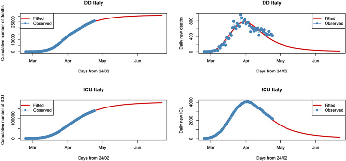
Fitted non‐linear robust models for the daily deaths and intensive care unit hospitalizations in Italy

FIGURE 2.

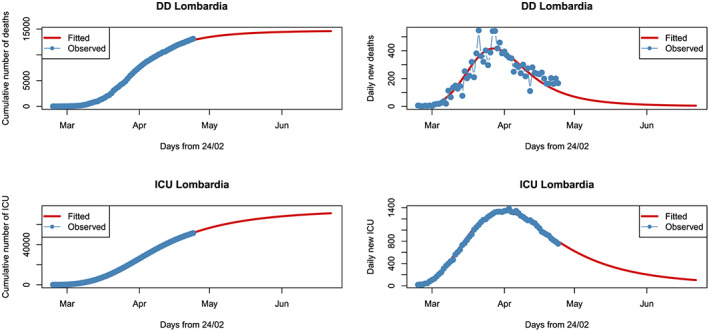
Fitted non‐linear robust models for the daily deaths and intensive care unit hospitalizations in Lombardia

The robust fits (Tsallis estimates and 95% confidence intervals) of the parameters e (inflection point) and d (upper asymptote) for the models are summarized in Tables 1 and 2 for DD and ICU, respectively. For DD Italy data, the model predicts an impressive total of more than 31k deceased at the end of the outbreak. According to the fitted model, the expected number of new deaths will be below 15 counts by the end of June. The inflection point is on April 5 (Day 42), whereas the fitted peak is on March 30. For what concerns ICU, the total expected number of ICU occupancy‐days is about 186k, whereas the inflection point is on April 8 (Day 45) and the peak on April 1. The number of ICU will decline at the same level as the end of February, at the very beginning of the outbreak in Italy, during the first days of July. Moving to Lombardia, the model estimates a total of about 148k deaths at the end of the epidemic, an inflection point on April 1 (Day 38), and a peak on March 27. For ICU counts, the total is about 76k occupancy‐days, the inflection point is on April 10 (Day 47), and the peak on March 31. By the end of May, the death tolls will go below 15 units, whereas by the end of June, the number of ICU will be well below 100.

TABLE 1.

Tsallis estimates (and 95% confidence intervals) of the parameters $\exp (e)$ and d for the models for daily deaths

	$\exp (e)$	IC $\exp (e)$	d	IC d
Italy DD	41.7	(40.5; 42.3)	31 185	(30 429; 31 942)
Lombardia DD	37.8	(37.4; 38.3)	14 740	(14 500; 14 980)

TABLE 2.

Tsallis estimates (and 95% confidence intervals) of the parameters $\exp \left(e\right)$ and d for the models for cumulative intensive care unit hospitalizations

	$\exp (e)$	IC $\exp (e)$	d	IC d
Italy ICU	45.0	(44.3; 45.8)	186 636	(185 880; 187 394)
Lombardia ICU	47.1	(46.6; 47.6)	75 693	(75 453; 75 932)

In order to assess the accuracy of the fitted models, some numerical studies have been carried out to investigate the actual sampling distribution of the proposed estimator. To this end, 10 000 samples have been drawn from the fitted model on Italy death data. The sampling distributions of the Tsallis estimates for (b, d, e, σ) are displayed in Figure 3. They all exhibit reasonable accuracy and precision, as confirmed by the comparison with the normal approximation to the distribution of the Tsallis estimator based on the fitted model.

FIGURE 3.

Sampling distribution of the Tsallis estimator for (b, d, e, σ). The solid curve is the normal approximation; the dashed curve is a kernel density estimate. The vertical dashed line gives the original estimate

3.1. Estimative density and simulation study

In the simplest instance of prediction, the object of inference is a future or a yet unobserved random variable Z. Let p _Z (z; θ) be the density of Z. The basic frequentist approach to prediction of Z, on the basis of the observed y from Y, consists in using the estimative predictive density function

$$p_e(z)=p_Z(z;\widehat{\theta }),$$

obtained by substituting the unknown θ with a consistent estimator, such as the Tsallis estimator or the MLE. Figure 4 reports the estimative predictive densities based on both the estimators for DD and the cumulative ICU. Note the Tsallis estimative predictive density is shifted on the right and exhibits larger variability.

FIGURE 4.

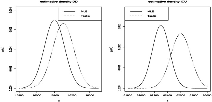
Estimative predictive densities based on the Tsallis and the ML estimators for DD (left) and cumulated ICU (right)

To compare the predictive performances of the Tsallis method with respect to the MLE, a simulation study has been performed, based on N = 10 000 Monte Carlo replications. Figure 5 reports the boxplots of point estimators of the mean μ(z, β) for the future observation z based on the predictive density estimated with the MLE and of the predictive density estimated with the Tsallis scoring rule, both under the central model (left) and under a contaminated model (right).

FIGURE 5.

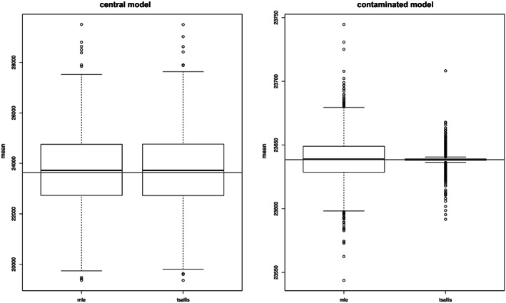
Boxplot of point estimators of the mean μ(z, β) for the future observation z under the central model (left) and under the contaminated model (right) based on the MLE and on the Tsallis scoring rule

We note that, under the central model, the two estimators present a similar behaviour. On the contrary, under the contaminated model, only the Tsallis estimator presents a robust performance. The values of the bias (and sd) are quite similar under the central model, contrary to the contaminated model.

3.2. Bayesian analysis

Mixing the robust procedure with the Bayesian approach allows us to include prior information (objective or subjective) on the parameters of the model. Moreover, the plots of the posterior distributions for the parameters of the model may be quite useful in practice since they are more informative than a simpler point or interval estimator. For instance, the marginal posterior distributions allow us to assign probabilities to intervals on the parameters.

Figure 6 gives the violin plots of the marginal posterior distributions for parameters of the model and the expected mean, both for DD and for ICU data, using the reference prior (Giummolé et al., 2019). The posterior medians (the white dots) for the upper asymptotes and the inflection points are consistent with the frequentist robust estimates. Note that the classical marginal posterior distribution shows too narrow tails with respect to robust posterior distributions, which, on the contrary, can take into account the actual large uncertainty in the available data.

FIGURE 6.

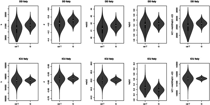
Marginal posterior distributions for the the parameters of model (1) and the expected mean value, with $\beta =(b,d,\exp (e),\log \sigma )$

4. FINAL REMARKS

To conclude, we believe that our procedure can constitute a useful statistical tool in modelling the Italian COVID‐19 contagion data. Indeed, the Tsallis robust procedures allow us to take into account the inevitable inaccuracy of the Italian COVID‐19 data, which are often underestimated. Moreover, an example is those deaths of patients who died with symptoms compatible with COVID‐19 but who have not had a symptom, or what has been described by many media regarding the growing number of elderly people who remain in their homes while needing to be hospitalized in intensive care. Thus, for these data, robust procedures are particularly useful since they allow us to deal at the same time with model misspecifications (with respect to the normal assumption, independence or homoscedasticity) and data reliability.

The estimation of the model and, as a consequence, the calculation of the expected asymptote and the inflection point are based on the assumptions that the adopted restrictions will not be subject to change. For these reasons, these fitted models cannot be used for predictive purposes, since it is not possible to predict how the data will change when the restrictions are modified at the end of the lockdown, scheduled for May 3. The day‐by‐day monitoring of the model fit stability will allow us to evaluate deviations from the actual lockdown situation with respect to the next reopening.

As a final remark, since the variables are daily counts, we will investigate the use of the Tsallis scoring rule in the context of non‐linear Poisson regression models.

Updates on the results and on the Italian regions may be found in the web page of the Robbayes‐C19research group: https://homes.stat.unipd.it/lauraventura/content/ricerca

In this web page also the R codes are available.

The reader is also pointed to the work of the StatGroup‐19 research group that models the mean function by using the five‐parameter Richards curve (Divino, Farcomeni, Jona Lasinio, Lovison, & Maruotti, 2020).

Girardi P, Greco L, Mameli V, et al. Robust inference for non‐linear regression models from the Tsallis score: Application to coronavirus disease 2019 contagion in Italy. Stat. 2020;9:e309. 10.1002/sta4.309

DATA AVAILABILITY STATEMENT

The data that support the findings of this study are available in GitHub repository at the Italian Protezione Civile account (pcm‐dpc/COVID‐19) and described in Morettini et al. (2020). These data were derived from the following resources available in the public domain: https://github.com/pcm-dpc/COVID-19/.

REFERENCES

- Basu, A. , Harris, I. R. , Hjort, N. L. , & Jones, M. C. (1998). Robust and efficient estimation by minimising a density power divergence. Biometrika, 85, 549–559. [Google Scholar]
- Bates, D. M. , & Watts, D. G. (2007). Nonlinear regression analysis and its applications. New York: Wiley. [Google Scholar]
- Dawid, A. P. , Musio, M. , & Ventura, L. (2016). Minimum scoring rule inference. Scandinavica Journal Statistics, 43, 123–138. [Google Scholar]
- Divino, F. , Farcomeni, A. , Jona Lasinio, G. , Lovison, G. , & Maruotti, A. (2020). Available at https://afarcome.altervista.org/growthGLM.pdf
- Farcomeni, A. , & Greco, L. (2015). Robust methods for data reduction. CRC Press, Boca Raton.
- Farcomeni, A. , & Ventura, L. (2012). An overview of robust methods in medical research. Statistical Methods in Medical Research, 21, 111–133. [DOI] [PubMed] [Google Scholar]
- Ghosh, M. , & Basu, A. (2013). Robust estimation for independent non‐homogeneous observations using density power divergence with applications to linear regression. Electrical Journal Statistics, 7, 2420–2456. [Google Scholar]
- Giummolé, F. , Mameli, V. , Ruli, E. , & Ventura, L. (2019). Objective Bayesian inference with proper scoring rules. Test, 28, 728–755. [Google Scholar]
- Huber, P. J. , & Ronchetti, E. M. (2009). Robust statistics. New York: Wiley. [Google Scholar]
- Mameli, V. , Musio, M. , & Ventura, L. (2018). Bootstrap adjustments of signed scoring rule root statistics. Communication Statistical Simulation Computation, 47, 1204–1215. [Google Scholar]
- Mameli, V. , & Ventura, L. (2015). Higher‐order asymptotics for scoring rules. Jounal Statististical Planning Information, 165, 13–26. [Google Scholar]
- Morettini, M. , Sbrollini, A. , Marcantoni, I. , & Burattini, L. (2020). COVID‐19 in Italy: Dataset of the Italian Civil Protection Department. Data in Brief, 105526. [DOI] [PMC free article] [PubMed] [Google Scholar]
- Pace, L. , Salvan, A. , & Sartori, N. (2011). Adjusting composite likelihood ratio statistics. Statistica Sinica, 21, 129–148. [Google Scholar]
- Ritz, C. , Baty, F. , Streibig, J. C. , & Gerhard, D. (2015). Dose–response analysis using R. PLoS ONE, 10(12), e0146021. [DOI] [PMC free article] [PubMed] [Google Scholar]
- Tsallis, C. (1988). Possible generalization of Boltzmann–Gibbs statistics. Journal Statististical Physics, 52, 479–487. [Google Scholar]
- Varin, C. , Reid, N. , & Firth, D. (2011). An overview of composite likelihood methods. Statistica Sinica, 21, 5–42. [Google Scholar]
- Ventura, L. , & Racugno, W. (2016). Pseudo‐likelihoods for Bayesian inference, Topics on methodological and applied statistical inference, series studies in theoretical and applied statistics, pp. 205–220. [Google Scholar]
Associated Data
This section collects any data citations, data availability statements, or supplementary materials included in this article.