Abstract
Isothermal hot compression tests of TC4–DT titanium alloy were performed under temperatures of 1203–1293 K and strain rates of 0.001–10 s−1. The purpose of this study is to develop a new high-precision modified constitutive model that can describe the deformation behavior of TC4–DT titanium alloy. Both the modified strain-compensated Arrhenius-type equation and the modified Hensel–Spittel equation were established by revising the strain rate. The parameters in the above two modified constitutive equation were solved by combining regression analysis with iterative methods, which was used instead on the traditional linear regression methods. In addition, both the original strain-compensated Arrhenius-type equation and Hensel–Spittel equation were established to compare with the new modified constitutive equations. A comparison of the predicted values based on the four constitutive equations was performed via relative error, average absolute relative error (AARE) and the correlation coefficient (R). These results show the modified Arrhenius-type equation and the modified Hensel–Spittel equation is more accurate and efficient with a similar prediction accuracy. The AARE-value of the two modified constitutive equation is relatively low under various strain rates and their fluctuation is small as the strain rate changes.
Keywords: constitutive equation, modified Arrhenius-type equation, strain rate, the Hensel–Spittel (HS) equation
1. Introduction
The deformation behavior of alloys is complicated at elevated temperatures. The deformation behavior of alloys is affected by many factors, including deformation conditions, work hardening (WH), dynamic recovery (DRV) and dynamic recrystallization (DRX) and phase transition. Constitutive equations can represent the material behaviors during deformation, and these equations can provide a fundamental understanding of the metal forming process [1,2]. Because a constitutive equation can relate stress and strain to the related conditions of temperature and strain rate, it plays a crucial role in numeric analysis, modeling and optimizing hot forming process parameters [3].
There were three main constitutive model categories: phenomenological constitutive models, physical-based constitutive models and artificial neural network constitutive models, which are used to predict the constitutive behavior of metals and alloys [4]. Moreover, the phenomenological constitutive models have a lesser number of material constants and can be easily calibrated [4]. Among all the phenomenological constitutive models, the strain-compensated Arrhenius-type model is widely used. Based on the flow stress of modified 9Cr–1Mo steel and SnSbCu Alloy, it was found that the strain-compensated Arrhenius-type model has higher prediction accuracy than the Johnson-Cook model and modified Zerilli–Armstrong model [5,6]. To predict the hot flow stress of 28CrMnMoV steel, Li et al. [7] found the prediction accuracy of the strain-compensated Arrhenius-type model is higher than that of modified Johnson Cook, modified Zerilli–Armstrong equation. For describing the hot deformation behavior, Wang found the strain-compensated Arrhenius-type model had the highest accuracy when compared to Johnson–Cook model, modified Johnson–Cook model, Zerilli–Armstrong model, modified Zerilli–Armstrong model and KHL model [8]. A similar result was obtained by developing constitutive models of 21–4 N heat resistant steel [9]. Moreover, the strain-compensated Arrhenius-type equation is most widely applied to describe the high-temperature flow behavior of metals and alloys [10,11,12,13,14,15,16,17,18]. These results mean that the strain-compensated Arrhenius-type model has a relatively strong predictive ability.
About the Arrhenius-type equation, Sellars and Tegart proposed that the sine-hyperbolic law can be used over a very wide range of stress [19], which is shown in Equation (1). The common effect of the temperatures and strain rates on the hot deformation behavior can be shown through the Zener–Hollomon parameter (Z) in an exponent-type equation, which is shown in Equation (2) [17].
| (1) |
| (2) |
where
| (3) |
| (4) |
| (5) |
where is the real strain rate (s−1), σ is the flow stress (MPa), T is the deformation temperature (K), Q is the activation energy (J·mol−1), R is the molar gas constant (8.3145 J·mol−1·K−1), A, n1, n, α and β are material constants. Moreover, α = β/n1.
Because there is no strain in the Arrhenius-type equation, the polynomial is employed to represent the influence of strain on material constants to establish the strain-compensated Arrhenius-type equation [20,21]. Moreover, the material constant α is used as an adjustable parameter to improve the predictive power of the Arrhenius-type equation [22,23,24,25]. Moreover, the exponent of the strain rate in the Arrhenius-type equation was revised to give an accurate and precise estimate for the flow stress of 42CrMo steel [20]. Wang et al. [26] proposed to obtain a more reasonable value of material constants by combining the iterative methods and regression analysis.
Regarding the Hensel-Spittel equation, it was proposed by Hensel and Spittel to describe the hot deformation behavior of metals and alloys [27]. Wei et al. [28] used Hensel-Spittel equation to describe the hot deformation of Mg–9Li–3Al–2Sr–2Y under the whole compression process. Claudimir J et al. [29] established the constitutive model of HSLA350/440 and DP350/600 steels based on the Hensel–Spittel equation. Flora et al. [30] used the Hensel–Spittel equation to predict the flow stress of TiAl–Mo alloys at high temperatures.
Because of its excellent physical and mechanical properties, TC4–DT titanium alloy is extensively adopted in a wide range of temperature applications. The elevated temperature can improve the plastic deformation ability of TC4–DT titanium alloy. Therefore, the hot deformation behaviors of TC4–DT titanium alloy have been investigated by some researchers.
Based on the flow stress of TC4–DT titanium alloy, Liu et al. [31] found there was low prediction accuracy of the strain-compensated Arrhenius-type flow stress equation at the higher strain rate. Peng et al. [32] obtained a similar result. In addition, based on hot deformation behavior of Ti2AlNb-based alloys, He et al. [33] performed a comparative study and found the Arrhenius-type equation was not suitable for the deformation with relatively higher strain rates. However, Tao et al. [34] found that the application of the strain-compensated Arrhenius-type equation is limited by its relatively low predicted accuracy at lower strain rates. In addition, for describing the hot tensile deformation Behavior of TC4–DT alloy (also named Ti–6Al–4V Alloy), Lin et al. [35] found the prediction accuracy of the Hensel–Spittel equation is higher than that of the strain-compensated Arrhenius-type equation.
In summary, because the strain-compensated Arrhenius-type equation cannot consider the effect of strain rates on stress relatively accurately, the accuracy under specific strain rates is relatively lower for predicting the flow stress of some metals and alloys, especially TC4–DT alloy. Although Peng et al. [32] improved the prediction accuracy of the strain-compensated Arrhenius-type equation by modifying the temperature and the exponent of strain rate under partial deformation conditions, they did not attempt to propose an effective method to establish a simpler constitutive equation. Moreover, based on the work of Lin et al. [35], the Hensel–Spittel equation may have a higher prediction accuracy for describing the hot compressed deformation behavior of TC4–DT alloy, which is also probably achieved by revising the Hensel–Spittel equation.
In present study, to predict the hot compressed flow stress of TC4–DT alloy, the new modified strain-compensated Arrhenius-type (ms–cA-type) and modified Hensel–Spittel (mHS) equation is developed by modifying the strain rate. Moreover, the two new modified constitutive equations are established by combining regression analysis with iterative methods, which is used instead of the traditional linear regression method. Meanwhile, both the original strain-compensated Arrhenius-type (os–cA-type) and original Hensel–Spittel (oHS) equation are established by the traditional method.
A comparative study has been made on the above four constitutive equations, which is used to prove the two modified constitutive equations are more accurate for prediction of the flow stress of TC4–DT alloy.
2. Materials and Methods
The flow stress data of TC4–DT alloy at elevated temperature is taken from the literature (Peng et al. [32]), which is shown in Table A1. The chemical composition (in wt%) of the titanium alloy is 6.20Al–4.1V–0.04Fe–0.017C–0.11O–(bal.) Ti. The microstructure is entirely homogeneous equiaxed α + β, consisting of 70% primary α phase with the average grain size 9 μm and transformed β with the secondary lamellar a thickness of 1.4 μm.
Cylindrical specimens with 12 mm in height and with 10 mm in diameter are prepared and their flat ends are recessed to a depth of 0.1 mm entrap the lubricant of graphite mixed with machine oil, which can minimize the frictions between the specimens and die. The isothermal hot compression tests were performed at temperatures of 1203, 1218, 1233, 1248, 1263, 1278 and 1293 K with strain rates of 0.001, 0.01, 0.1, 1 and 10 s−1. The isothermal hot compression tests of the titanium alloy were conducted on a Gleeble-1500 thermo-simulation system (Dynamic Systems Inc., Poestenkill, NY, USA). The specimen was heated to the deformation temperature at a rate of 10 K/s and held for 3 min to eliminate the thermal gradients.
3. Results
To predict the flow stress of TC4–DT titanium alloy, Peng et al. [32] determined two sets of material constants in the original strain-compensated Arrhenius-type equations based on different phase regions, and they modified the original constitutive equation under partial deformation condition. These results mean that the flow stress curves of TC4–DT titanium alloy obtained by Peng et al. [32] are more complicated. Therefore, the experimental data collected by Peng et al. [32] is used in the current study, which is used to prove a stronger predictive ability of the new modified constitutive equations and the authenticity of results.
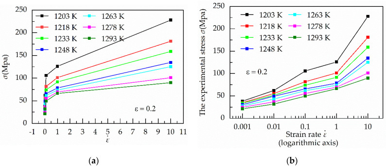
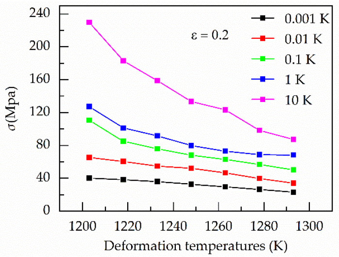
Figure 1 shows the relationship between vs. the mean of σ and vs. σ under the strain of 0.20 and various temperatures. It is easily found a strong nonlinear relationship between σ and at various temperatures. Moreover, as the value of strain rate increases from 1 to 10 s−1, the stress increases sharply, especially below 1273 K. Figure 2 shows the relationship between temperatures and stress under the strain of 0.20 and various strain rates. When the value of the strain rate is below 1 s−1, the change of stress with temperature is relatively stable. However, under the strain of 10 s−1, the stress decreases sharply as the temperature increases.
Figure 1.
Relationship between (a) vs. the mean of σ; (b) vs. σ under the strain of 0.20 and various deformation temperatures.
Figure 2.
Relationship between deformation temperatures and stress under the strain of 0.20 and various strain rates.
At hot temperature, the flow stress of metals and alloys is dependent on the interaction between them the work hardening and the dynamic softening mechanisms between the work hardening and the dynamic softening mechanisms. As the strain rate increases, the time required to reach the same strain becomes shorter. Moreover, the dynamic softening mechanisms become increasing insufficient, including the dynamic recovery (DRV) and dynamic recrystallization (DRX). Therefore, stress increase with the rise of the strain rate, especially above 1 s−1 in Figure 1b. In contrast, the increase in temperature promotes dynamic recovery (DRV) and dynamic recrystallization (DRX). At the higher stain rate, the softening effect of temperature becomes increasing prominent, especially at 1293 K in Figure 2.
In Figure 1 and Figure 2, differences in strain rates lead to different trends in stress. Therefore, these results mean the strain rate has a significant influence on stress, especially under the higher strain rate.
Based on the above result, revising the strain rate is used to improve the accuracy of the constitutive equation. Therefore, the new modified strain-compensated Arrhenius-type (ms–cA-type) equation and the modified Hensel–Spittel (mHS) equation is established. Moreover, it is also established the original strain-compensated Arrhenius-type (os–cA-type) equation and the original Hensel–Spittel (oHS) equation. The four constitutive equations are used to predict the flow stress of TC4–DT titanium alloy under temperatures of 1203–1293 K and strain rates of 0.001–10 s−1. The different constitutive equations are compared to prove that the accuracy of the modified equation is higher.
3.1. Establishing the Original Strain-Compensated Arrhenius-Type (os–cA-type) Equation
The relationship between deformation parameters at elevated temperature can be expressed by the original Arrhenius-type equation, which is shown in Equation (1). The hyperbolic sine model in the Arrhenius-type equation gives better approximations for the flow stress of the TC4–DT titanium alloy.
Material constants are solved based on experimental data from the isothermal hot compression tests. The strain of 0.30 is taken as an example to introduce the procedures of solving material constants.
Substituting Equations (4) and (5) in Equation (1), respectively gives:
| (6) |
| (7) |
Taking the logarithm of both sides of Equations (6) and (7), respectively yields:
| (8) |
| (9) |
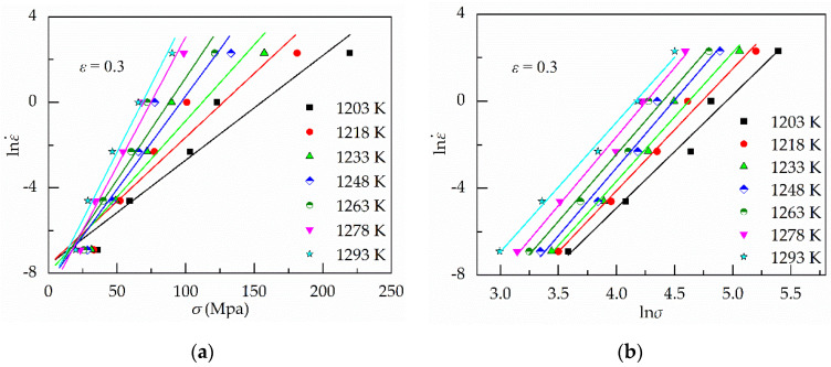
Then, it is obtained that two groups of straight lines based on Equations (8) and (9), as shown in Figure 3a,b, respectively. The values of n1 and β are the average value of the slope of the fitting lines in the lnσ–ln and σ–ln plots, which were 5.9160 and 0.0871, respectively. Then, the value of α is 0.0147 based on α = β/n1. Moreover, the values of ασ varied from 0.29 to 3.23 under the strain of 0.30. Therefore, it is reasonable to choose the constitutive equation under all the strain levels.
Figure 3.
Results of regression analysis for determining α. (a) Relationship between σ–ln; (b) relationship between lnσ–ln.
For all the strain levels, Equation (1) can be written as:
| (10) |
Taking the logarithm of both sides of Equation (10) gives:
| (11) |
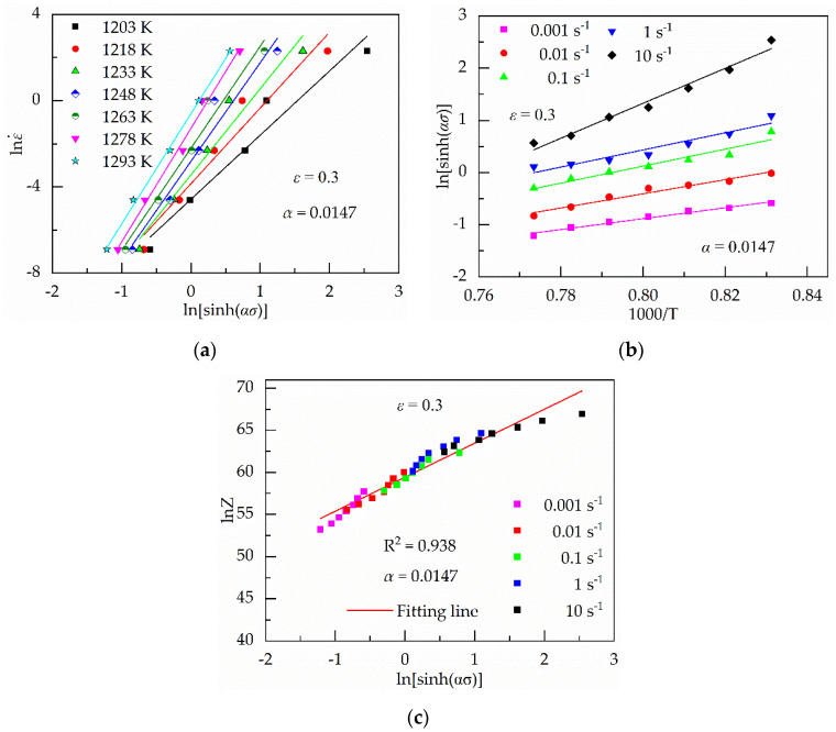
The value of n can be obtained from the average slope of the lines in ln–ln[sinh(ασ)] plots, as shown in Figure 4a.
Figure 4.
Results of regression analysis based on = 0.0147. (a) Relationship between ln[sinh(ασ)]–ln; (b) relationship between 1000/T–ln[sinh(ασ)]; (c) relationship between ln[sinh(ασ)]–lnZ.
Because the value of ln[sinh(ασ)] is approximately 1000 times the value of 1/T, 1000/T is used instead of 1/T to obtain a more accurate result. When 1000/T is used, the unit of Q becomes kJ·mol−1.
For a particular strain rate, Equation (12) can be derived based on Equation (11), as follows:
| (12) |
Therefore, the value of Q can be gained from the average slope of the lines in ln[sinh(ασ)]–1000/T under various strain rates, as shown in Figure 4b.
Substituting Equation (2) in Equation (10) and taking the logarithm of both sides of Equation (10) give:
| (13) |
Based on Equation (13), it is easily found that the relationship between ln[sinh(ασ)] and lnZ is linear. Moreover, the value of lnA is the lnZ-intercept of the fitting lines in the ln[sinh(ασ)]–lnZ plots when the value of ln[sinh(ασ)] is zero, as shown in Figure 4c. The values of n, Q and lnA are 4.31, 646.50 and 59.43, respectively.
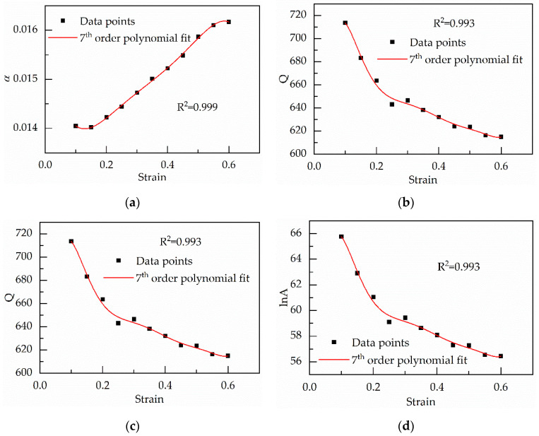
In summary, the values of material constants α, n, Q and lnA are obtained under a single strain, namely ε = 0.30. However, when the strain is different, the values of the material constants will change [21]. The constitutive equation is established based on strain range from 0.10 to 0.60 at an interval of 0.05. The above solving process is repeated to obtain material constants under various strains. By adjusting the order of the polynomial, it is found that a seventh order of the polynomial is employed to represent the influence of strain on material constants with a very good correlation and generalization, which is shown in Figure 5 and Equation (14) [35]. Moreover, the values of multinomial coefficients are shown in Table 1.
| (14) |
Figure 5.
Variation of (a) α; (b) n; (c) lnA; (d) Q with true strain represented by a 7th order of the polynomial.
Table 1.
Coefficients of the polynomial for α, n, Q and lnA.
| α | n | Q | lnA |
|---|---|---|---|
| a0 = 0.0136 | N0 = 5.024 | Q0 = 425.153 | A0 = 39.642 |
| a1 = 0.0236 | N1 = −5.757 | Q1 = 9463.639 | A1 = 860.817 |
| a2 = −0.3988 | N2 = 72.989 | Q2 = −113,579.0 | A2 = −10,345.921 |
| a3 = 2.9127 | N3 = −649.946 | Q3 = 647,939.428 | A3 = 58,956.037 |
| a4 = −10.4516 | N4 = 2802.387 | Q4 = −2.029 × 10⁻⁶ | A4 = −184,298.5 |
| a5 = 19.8532 | N5 = −6137.141 | Q5= 3.575 × 10⁻⁶ | A5 = 324,376.105 |
| a6 = −19.0393 | N6 = 6620.972 | Q6= −3.332 × 10⁻⁶ | A6 = −302,056.1 |
| a7 = 7.2107 | N7 = −2796.638 | Q7 = 1.279 × 10⁻⁶ | A7 = 115,906.977 |
When the materials constant can be evaluated based on Equation (14), the flow stress can be predicted from Equation (15) [14,32], which is derived from Equations (1), (2) and (5).
| (15) |
3.2. Establishing the Modified Strain-Compensated Arrhenius-Type (ms–cA-type) Equation
The modified strain-compensated Arrhenius-type (ms–cA-type) equation is developed by revising the strain rate in the original strain-compensated Arrhenius-type equation. Namely, the constitutive equation is modified by using an effective strain rate instead of real strain rate again. The modified Arrhenius-type equation is shown in Equation (16).
| (16) |
where is the effective strain rate (s−1), σ is the flow stress (MPa), T is the deformation temperature (K), Q is the activation energy (J·mol−1), R is the molar gas constant (8.3145 J·mol−1·K−1), A, α, n and m are material constants.
First, material constants are obtained to establish the modified strain-compensated Arrhenius-type equation. Because material constants A, α, n, m and Q change with strain, it is necessary to solve material constants under various strain. After obtaining material constants under different strain, the effective strain rate can be determined.
3.2.1. Determining Material Constants
Wang et al. [26] proposed material constants in the Arrhenius-type equation were solved by combining iterative methods with regression analysis. In the prevent study, the same method is used to solve the material constants in the modified Arrhenius-type equation. During solving material constants, A, α, n, m and Q, the real strain rate is used instead of the effective strain rate in Equation (16). Namely, substituting in Equation (16) gives:
| (17) |
Taking the logarithm of both sides of Equation (17) gives:
| (18) |
Rearranging gives:
| (19) |
where sinh−1 is the inverse function of sinh.
1000/T is used instead of 1/T to obtain a more accurate result again. Therefore, the unit of Q becomes kJ·mol−1.
Based on Equations (18) and (19), Equations (20) and (21) is established, respectively.
| (20) |
| (21) |
Substituting Equations (20) and (21) in Equations (18) and (19), respectively gives:
| (22) |
| (23) |
If α is determined, the n, Q and A (b1, b2 and b3) will be obtained by performing multiple linear regression on Equation (22). Similarly, if n, Q and A are determined, the α (c) will be obtained by performing linear regression on Equation (23). Therefore, iterative methods can be used to solve material constants.
Based on the above analysis, it is used that a new method combines regression analysis with iterative methods. About the new method, first, the initial guess of α is determined to solve x1 in Equation (23). Second, the approximation of n, Q and A is determined by performing multiple linear regression on Equation (22). Third, n, Q and A obtained in the second step are substituted in Equation (21) to determine y2, and then the approximation of α is determined by performing linear regression on Equation (23). Fourthly, the approximation of α from one iteration is the input of the next to iterate Equation (22) and (23) until a stopping criterion is met. Finally, it is obtained the convergence values of n, Q, A and α under a single strain.
The above four steps are repeated for solving material constants under different strain. When the stopping criterion is established based on the predicted stress under all strain, it is used to obtain the convergence values of n, Q, A and α under various strain. The solution process under a single strain is as follows:
The strain of 0.30 is still taken as an example to introduce the procedures of solving material constants n, Q, A and α under a single strain. The real strain rate is used to replace the effective strain rate during determining material constants.
At first, the initial guess of α is the value of α in the original Arrhenius-type equation under strain of 0.30. Namely, the initial guess of α is equal to 0.0147. Next, it is needed to determine the value of x1. At a special strain, there are seven different deformation temperatures (1203, 1218, 1233, 1248, 1263, 1278 and 1293 K) and five different values of strain (0.001, 0.01, 0.1, 1 and 10 s−1), which can be obtained based on the selected experimental data points. Namely, there are thirty-five experimental data points at a special strain. The set of x1-values can be obtained based on the experimental data points and Equation (20). The multiple linear regression is performed based on Equation (22), where x1, x2 and x3 are the independent variables, y1 is the dependent variable and b1, b2 and b3 are the unknown parameters.
Newton’s method is used to perform multiple linear regression. For Newton’s method, the initial value of the unknown parameters is needed. The initial guess of b1, b2 and b3 are 4.31, 646.50 and 59.43, respectively. After finishing multiple linear regression, it is obtained that the approximate value of b1, b2 and b3 are 3.99, 597.50 and 54.72, respectively.
Then, the set of y2-values is obtained by substituting the value of b1, b2 and b3 in Equation (21). Linear regression can be performed based on Equation (23). During linear regression, Equation (23) is the regression model, x4 is the independent parameters, y1 is the dependent variable and c is the unknown variables. Newton’s method is still used to perform linear regression and the initial guess of α is still equal to 0.0147. After finishing linear regression, it is obtained that the approximate value of c (α) is 0.0146. To date, the approximate values of n, Q, A and α are obtained. Namely, it is obtained the results of the first iteration, which is shown in Equation (24).
| (24) |
The approximate value of α is the input of the next iteration to continue to iterate Equations (22) and (23). After the 253rd iteration, the approximate values of b1, b2, b3 and c are 5.86, 586.27, 80.10 and 1.927 × 10⁻⁴, respectively. Therefore, a new result is obtained, which is shown in Equation (25). The strain rate is not modified in Equations (24) and (25).
| (25) |
MATLAB software is used for programming and the nlinfit function is called to conduct regression analysis based on Newton’s method.
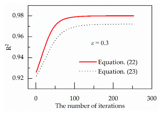
In the above iterative process, the same number of data points and the same regression model are used in regression analysis and the prediction accuracy can be verified by the coefficient of determination (R2), which is shown in Equation (26) [36]. The higher the R2-value, the higher the prediction accuracy. Figure 6 shows R2-values of Equations (22) and (23) keep increasing with increasing the number of iterations, which means the prediction accuracy is continuously improved with increasing the number of iterations. Therefore, the prediction accuracy of Equation (25) is higher.
| (26) |
where Ei is the experimental data, Pi is the predicted value obtained from the constitutive equation, is the mean value of Ei and N is the total number of data employed in the investigation.
Figure 6.
Variation of R2 of Equations (22) and (23) with iterations.
To date, it is shown the process of solving the material constants under a single strain. Then the stopping criterion is determined to obtain material constants in the strain range from 0.10 to 0.60 at an interval of 0.05.
About the stopping criterion, average absolute relative error (AARE) is an unbiased statistical parameter that is calculated via a term-by-term comparison of the relative error [12], as shown in Equation (27). Moreover, AARE is always used to verify the accuracy of the constitutive models. Therefore, AARE-value is obtained based on the predicated stress in the strain range from 0.10 to 0.60 at an interval of 0.05. Moreover, the stopping criterion is the error of AARE from the previous iteration to this one, as shown in Equation (28).
| (27) |
where Ei is the experimental data, Pi is the predicted value obtained from the constitutive equation and N is the total number of data points.
| (28) |
where AAREi and AAREi−1 is the average absolute relative error from the ith and i − 1th iteration.
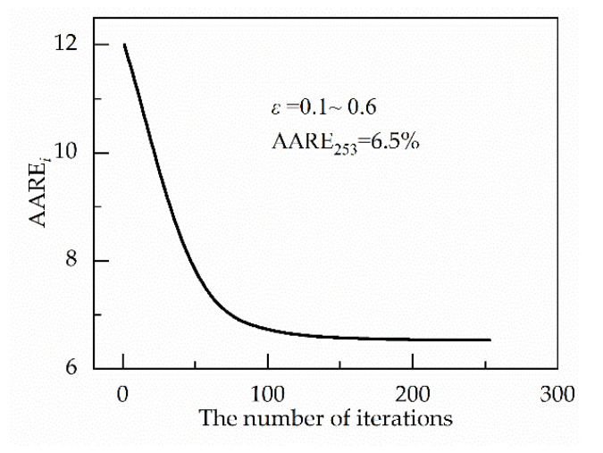
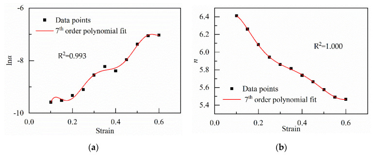
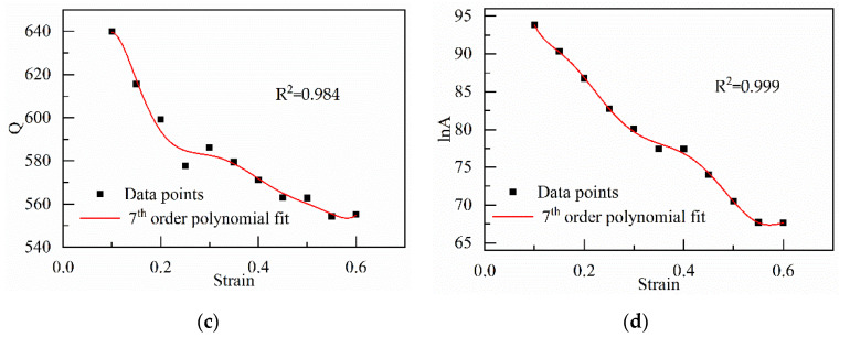
The value of AAREi changes with the number of iterations, as shown in Figure 7. After the 253rd iteration, the stopping criterion is met. AARE235 is equal to 6.53%. It is also obtained that material constants under strain in the range from 0.10 to 0.60. In addition, a seventh-order polynomial is used to describe the relationship between material constants and strain, which is shown in Figure 8. The coefficients of the polynomial functions are given in Table 2. Because the values of α are far less than 10−3, the logarithm of α is used to describe the correlation between the strain and it.
Figure 7.
Variation of average absolute relative error (AARE)i with iterations.
Figure 8.
Variation of (a) lnα; (b) n; (c) ln A; (d) Q with true strain represented by a 7th order of the polynomial.
Table 2.
Coefficients of the polynomial for α, n, Q and lnA in the ms–cA-type equation.
| lnα | n | Q | lnA | |
|---|---|---|---|---|
| a0 = −33.2764 | N0 = 5.539 | Q0 = 168.423 | A0 = 181.345 | E0 = −0.0769 |
| a1 = 683.8600 | N1 = 26.621 | Q1 = 14,166.731 | A1 = −2463.403 | E1 = 0.9819 |
| a2 = −7783.1519 | N2 = −278.626 | Q2 = −161,429.97 | A2 = 28,124.806 | |
| a3 = 45,443.6811 | N3 = 1260.164 | Q3 = 904,869.178 | A3 = −169,711.35 | |
| a4 = −147,592.0013 | N4 = −3006.507 | Q4= −2.811 × 10⁻⁶ | A4 = 569,436.405 | |
| a5 = 269,494.6845 | N5 = 3912.161 | Q5= 4.936 × 10⁻⁶ | A5 = −1.068 × 10⁻⁶ | |
| a6 = −258,493.9747 | N6 = −2643.084 | Q6= −4.593 × 10⁻⁶ | A6 = 1.046 × 10⁻⁶ | |
| a7 = 101,249.5269 | N7 = 743.522 | Q7 = 1.763 × 10⁻⁶ | A7 = −415,487.31 |
3.2.2. Determining Effective Strain Rate
By the above process, it is obtained the value of n, Q, A and α under the strain range from 0.10 to 0.60 at an interval of 0.05. After that, the effective strain rate is solved. The process of solving is as follows:
At a special strain rate, there are seven different deformation temperatures (1203, 1218, 1233, 1248, 1263, 1278 and 1293 K) and eleven different values of strain (0.10, 0.15, 0.20, 0.25, 0.30, 0.35, 0.40, 0.45, 0.50, 0.55 and 0.60), which can be obtained based on the selected experimental data points. Namely, there are seventy-seven experimental data points at a special strain rate. The values of strain, stress, and deformation temperatures in an experimental data point are substituted in Equation (17). Moreover, it is obtained a value of strain rate. Finally, based on the seventy-seven experimental data points, the seventy-seven values of strain rates can be obtained. Because there are errors in the process of solving the material parameters, there are differences between the seventy-seven values of strain rates. Based on least squares, the mean of the seventy-seven values of strain rates is used as the effective strain rate at the special strain rate, which is shown in Equation (29).
| (29) |
where is the effective strain rate under a special strain rate; ε is the strain; nε, Qε, Aε and αε are the corresponding material constants under the strain ε; T is the deforming temperature; σε,T is the corresponding experimental stress under the strain ε, the temperature T and the special strain rate; and N is the total number of data points under the special strain rate.
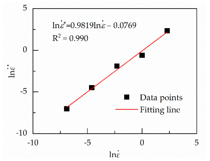
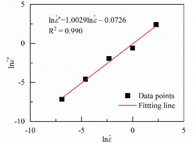
The corresponding at different can be obtained by repeating the above process. Because the maximum of the real and effective strain rate is ten times more than the minimum values, the logarithm of and is used to describe their correlation, which is shown in Equation (30) and Figure 9. The coefficients of the linear functions are given in Table 2.
| (30) |
Figure 9.
Relation between ln and ln.
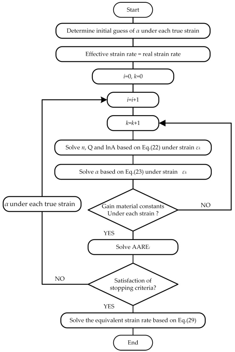
In summary, material constants and effective strain rate are determined based on the above solution procedure, which is shown in Figure 10. The modified Arrhenius-type equation is derived from Equations (16) and (30), as shown in Equation (31).
| (31) |
Figure 10.
Flow chart of establishing the modified strain-compensated Arrhenius-type equation.
To simplify form of Equation (31), Z* is used instead of Z in Equation (2) While in Equation (30) is used instead of in Equation (2). Therefore, a new equation is developed, as follows:
| (32) |
Substituting Equation (32) in Equation (31) and rearranging give:
| (33) |
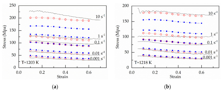
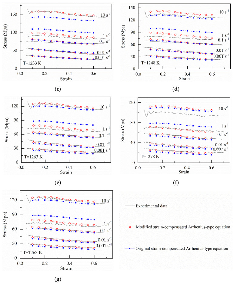
When the parameters in Equation (33) can be evaluated based on Equation (34) and Table 2, the flow stress can be predicted, which is shown in Figure 11.
| (34) |
Figure 11.
Comparison between the experimental and predicted stress by the original and modified strain-compensated Arrhenius-type equations at (a) 1203 K; (b) 1218 K; (c) 1233 K; (d) 1248 K; (e) 1263 K; (f) 1278 K; (g) 1293 K.
3.3. Establishing the Original Hensel–Spittel (oHS) Equation
Hensel and Spittel proposed a constitutive equation (namely HS equation) to predict the flow curves of alloy [27], which is shown in Equation (35).
| (35) |
where α, A, m1, m2, m3, m4, m5, m6, m7 and m8 are material parameters. Generally, m7 and m8 are neglected.
Taking the logarithms on both sides of Equation (35) gives:
| (36) |
About Equation (36), α is a function of stain. The values of α can be gained based on the seventh polynomial related to strain, which is shown in Figure 5a [37]. Other material parameters can be obtained by multiple linear regression, which is listed in Table 3.
Table 3.
Material parameters obtained by the traditional method.
| A | m 1 | m 2 | m 3 | m 4 | m 5 | m 6 |
|---|---|---|---|---|---|---|
| 3,199,230.981 | −0.0113 | 0.1064 | 0.2329 | 0.0114 | −0.0008 | 0.5115 |
3.4. Establishing the Modified Hensel–Spittel (mHS) Equation
In the present study, the modified Hensel–Spittel (mHS) equation is established by using the effective strain rate instead of the real strain rate , which is shown in Equation (37).
| (37) |
where the α, A, m1, m2, m3, m4, m5, m6, m7 and m8 are material parameters, α is a fixed value independent of strain, is a function of .
About solving material parameters in mHS equation, there is a process similar to solving the parameters in the modified strain-compensated Arrhenius-type equation. At first, the real strain rate is used instead of the effective strain rate in Equation (37). Namely, the modified Hensel–Spittel (mHS) equation is transformed into Equation (35). Next, the material parameters can be solved by combining regression analysis with iterative methods. Because it is needed to perform regression analysis, Equation (35) is transformed into Equation (36).
Rearranging Equation (36) gives:
| (38) |
Based on Equations (36) and (38), Equations (39) and (40) are established, respectively.
| (39) |
| (40) |
Substituting Equations (39) and (40) in Equations (36) and (38), respectively gives:
| (41) |
| (42) |
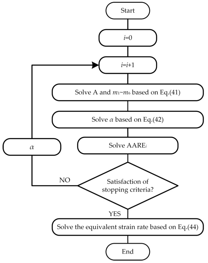
In summary, Equation (37) is transformed into two linear equations, namely Equation (41) and Equation (42). If the material parameter α can be determined, the other material parameters will be obtained by performing multiple regression analysis based on Equation (41). Similarly, if the parameters m1~m6 can be determined, the material parameter α will be obtained by performing regression analysis based on Equation (42). A new iterative process is established based on the above analysis, which is shown in Figure 12. The material parameters can be solved by combining regression analysis with iterative methods. The initial guess of α is 0.0147 for iterative methods. The stopping criterion is still Equation (28). When the stopping criterion is met, the material parameters m1~m6, α, and A can be gained, which is shown in Table 4.
Figure 12.
Flow chart of establishing the modified Hensel–Spittel (mHS) equation.
Table 4.
Material parameters in the modified Hensel–Spittel (mHS) equation.
| α | A | m 1 | m 2 | m 3 | m 4 | m 5 | m 6 | e | e 1 |
|---|---|---|---|---|---|---|---|---|---|
| 0.0003 | 342.914 | −0.0075 | −0.0863 | 0.16784 | −0.0131 | −0.0005 | 0.2511 | 2.7183 | −0.0863 |
After that, the effective strain rates can be solved based on the material parameters. At first, the real strain rate is separated from the constitutive equation. Rearranging Equation (35) gives:
| (43) |
Next, based on least squares, it is solved the optimal of the strain rate, which is used as the effective strain rate. At a special strain rate, there are seventy-seven experimental data points. The values of strain, stress, and deformation temperatures in experimental data points are substituted in Equation (43). As a result, it is obtained the seventy-seven values of strain rates. Based on least squares, the mean of the seventy-seven values of strain rates is used as the effective strain rate at the special strain rate , as follows:
| (44) |
where the α, A, m1, m2, m3, m4, m5 and m6 are material parameters, T is temperature, is the strain, is stress under T, and a special strain rate , N is the total number of data employed in the investigation, and is the corresponding the effective strain rate at a special strain rate .
The corresponding at different can be obtained by repeating the above process. Then, it is established a relationship between the strain rate and the effective strain rate. The linear equation can be used to describe the relationship between and , which is shown in Equation (45) and Figure 13. In Equation (45), the values of e0 and e1 are 0.1668 and −0.0863, respectively.
| (45) |
Figure 13.
Relation between ln and ln in the modified Hensel–Spittel (mHS) equation.
Rearranging Equation (45) gives:
| (46) |
where e = exp(e0).
Finally, the new modified constitutive equation is developed by using the effective strain rate instead of the strain rate in the original constitutive equation. Substituting Equation (46) in Equation (37) gives:
| (47) |
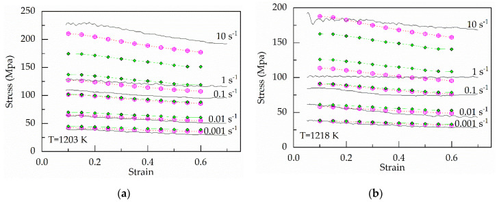
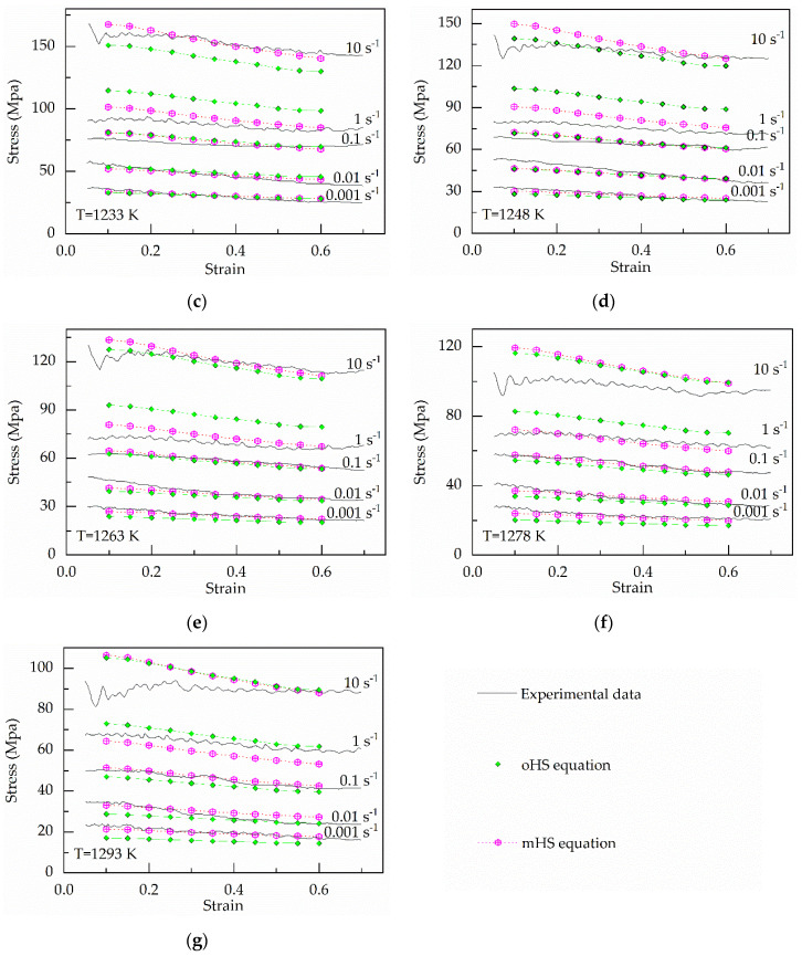
In summary, the modified Hensel–Spittel (mHS) equation is established, which is shown in Equation (47). The material parameters are listed in Table 4. The predicted stress the original Hensel–Spittel (oHS) equation and the modified Hensel–Spittel (mHS) equation is shown in Figure 14.
Figure 14.
Comparison between the experimental and predicted stress from the original Hensel–Spittel (oHS) equation and the modified Hensel–Spittel (mHS) equation at (a) 1203 K; (b) 1218 K; (c) 1233 K; (d) 1248 K; (e) 1263 K; (f) 1278 K; (g) 1293 K.
4. Discussion
In the present study, it was established two original and two modified constitutive equations. The two original constitutive equations are the original strain-compensated Arrhenius-type (os–cA-type) equation, and the original Hensel–Spittel (oHS) equation, respectively. Moreover, the two modified constitutive equations include the modified strain-compensated Arrhenius-type (ms–cA-type) equation and the modified Hensel–Spittel (mHS) equation.
A comparative study was made on the above four constitutive equations and their predictability was evaluated in terms of the correlation coefficient (R), average absolute relative error (AARE) and the relative error (RE) and the average root mean square error (RMSE). The correlation coefficient (R) is shown in Equation (48).
| (48) |
where Ei is the measured stress, Pi is the estimated stress, and are the mean values of measured and estimated flow stresses, respectively.
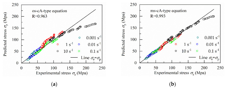
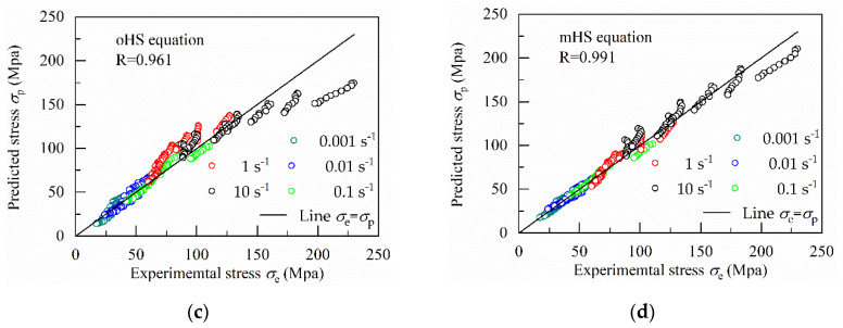
The correlation coefficient (R) is a statistical measure of the strength of the linear relationship between two variables. It is assumed that the predicted stress σp is equal to the experimental stress σe. There will be a linear relationship between σp and σe, namely σp = σe, when σp = σe, R = 1. As the prediction accuracy decreases, the linear relationship between σp and σe becomes weaker and the value of R also decreases. Therefore, the correlation coefficient (R) can be used as a measure of prediction accuracy by verifying the strength of the linear relationship between σp and σe. Figure 15 shows the correlation between the experimental stress and predicted flow stress values from the different constitutive equations.
Figure 15.
Correlation between the experimental stress and predicted flow stress values from (a) original strain-compensated Arrhenius-type (os–cA-type) equation; (b) modified strain-compensated Arrhenius-type (ms–cA-type) equation; (c) original Hensel–Spittel (oHS) equation; (d) modified Hensel–Spittel (mHS) equation.
In Figure 15, the R-value of the modified strain-compensated Arrhenius-type (ms–cA-type) equation (0.993) are the maximum, which is followed by the modified Hensel–Spittel (mHS) equation (0.991), the original strain-compensated Arrhenius-type (os–cA-type) equation (0.963) and the original Hensel–Spittel (oHS) equation (0.961).
Meanwhile, the straight line σp = σe are introduced into Figure 15, which is used to show the difference between these constitutive equations. When σp = σe, the data point is located on the straight line σp = σe. The distance from the data point to line σp = σe increases as the error value between σp and σe increases.
From Figure 15, it is easily found that the data point under the strain rate of 10 s−1 has the farthest distance to the straight line σp = σe, which means the corresponding error is the largest. However, the flow stress is different as temperatures, strain and strain rates changes. The same error between the experimental and predicted stress may mean different results for two unequal experimental stress values. In statistics, normalization can overcome the above shortcomings. Therefore, as a normalized unbiased statistical parameter, the average absolute relative error (AARE) is used to verify the predictability of the four constitutive equations. The smaller the value of AARE, the higher the accuracy of the constitutive equation.
The modified strain-compensated Arrhenius-type equation has the smallest AARE-value (4.67%) when compared to the AARE-value of the modified Hensel–Spittel (mHS) equation (5.31%), the AARE-value of the original strain-compensated Arrhenius-type (os–cA-type) equation (10.16%), the AARE-value of the original Hensel–Spittel (oHS) equation (10.65%). The AARE-value of any original constitutive equation (namely, the os–cA-type equation and the oHS equation) is more than twice that of the corresponding modified constitutive equation (namely, the ms–cA-type equation and the mHS equation).
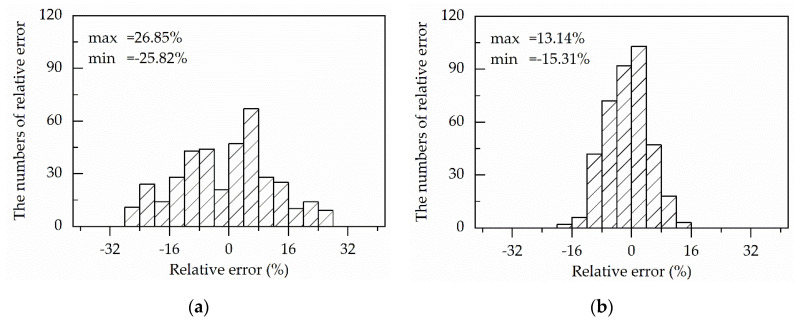
As a statistical parameter, the relative error is commonly employed to show the distribution of errors between the experimental and predicted values [6]. The relative error is calculated by comparing the data points and predictions via a term-by-term, which is shown in Equation (49).
| (49) |
where Ei and Pi still are the experimental data and is the predicted value, respectively. Moreover, the results are shown in Figure 16.
Figure 16.
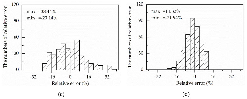
Statistical analysis of the relative error from (a) the original strain-compensated Arrhenius-type (os–cA-type) equation; (b) modified strain-compensated Arrhenius-type (ms–cA-type) equation; (c) original Hensel–Spittel (oHS) equation; (d) modified Hensel–Spittel (mHS) equation.
The relative errors gained from modified strain-compensated Arrhenius-type (ms–cA-type) equation and the modified Hensel–Spittel (mHS) equation vary from −15.31% to 13.14% and −21.94% to 11.32%, respectively, whereas it is in the range of −25.82% to 26.85% for the modified strain-compensated Arrhenius-type (ms–cA-type) equation and −23.14% to 38.44% for the modified Hensel–Spittel (mHS) equation.
Moreover, 90.65% and 87.80% of the numbers of relative errors of the modified strain-compensated Arrhenius-type (ms–cA-type) equation and the modified Hensel–Spittel (mHS) equation locate between RE-values of −10% and 10%. Compared with the two modified constitutive equation, the percentage of the RE-number of the original strain-compensated Arrhenius-type (os–cA-type) equation and the original Hensel–Spittel (oHS) equation are 57.40% and 55.84%, respectively, in the same RE-values range from −10% to 10%.
In addition, the average root mean square error (RMSE) is a statistical measure for model performance evaluation [14,38], which is used to compare the four constitutive equations further. The expression of RMSE is as follows:
| (50) |
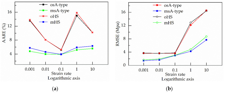
where RMSE is the average root mean square error, Ei is the experimental data and Pi is the predicted value obtained from the model, and N is the total number of data employed in the investigation. Regarding the four constitutive equations, the results of RMSE-values are very similar to the results of ARRE-values. The RMSE-value of any original constitutive equation (namely, the os–cA-type equation and the oHS equation) is more than twice as big as the corresponding modified corresponding constitutive equation (namely, the ms–cA-type equation and the mHS equation).
In addition, RMSE-values and AARE-values under a single strain rate can be used to explain the effect of stain rates on the prediction accuracy of the four constitutive equations.
From Figure 17, with increasing the strain rate, RMSE-values of the two original constitutive equation (namely, the os–cA-type equation and the oHS equation) change little in the beginning, but their AARE-values decrease sharply. The reason is that the stress increases with the increase of strain rate, which is shown in Figure 1. When the strain rate reaches 0.1 s−1, every original constitutive equation obtains the smallest AARE-value, which is slightly higher than the AARE-value of the any modified constitutive equations (namely, the ms–cA-type equation and the mHS equation). As the stain rate continues increasing, RMSE-values of the two original constitutive equations increase sharply, but their AARE-values increases first and then decreases. Because the increase ratio of RMSE is higher first and then lower than that of the experimental stress, and the values of stress rise sharply as the value of the strain rate increases from 1 to 10 s−1, which is shown in Figure 1. AARE-values of the two original constitutive equations reaches the maximum when the strain rate is one per second.
Figure 17.
The relationship between the strain rate and (a) AARE; (b) RMSE obtained by the original strain-compensated Arrhenius-type (os–cA-type) equation, the modified strain-compensated Arrhenius-type (ms–cA-type) equation, the original Hensel–Spittel (oHS) equation and the modified Hensel–Spittel (mHS) equation.
Although RMSE-values of the two modified constitutive equations (namely, the ms–cA-type equation and the mHS equation) also increase as the strain rate increases, their AARE-values change relatively little. The reason is that the RMSE-value of the two modified constitutive equation has the increasing ratio similar to the experimental stress. Moreover, under various strain rates, RMSE-value of every modified constitutive equation is lower than that of any original constitutive equation. Therefore, the modified constitutive equations can have higher accuracy and reflect the effect of strain rate on stress more accurately.
In sum, the results of the R, AARE, RMSE and RE of the four constitutive equations are listed in Table 5. Based on the above result, it is found that the original strain-compensated Arrhenius-type (os–cA-type) equation and the original Hensel–Spittel (oHS) equation have a similar and relatively lower prediction accuracy. The prediction accuracy of the modified strain-com Arrhenius-type constitutive equation is the highest, which is slightly higher than the prediction accuracy of the modified Hensel–Spittel (mHS) equation.
Table 5.
R, AARE, RMSE and RE of the original strain-compensated Arrhenius-type (os–cA-type) equation, the modified strain-compensated Arrhenius-type (ms–cA-type) equation, the original Hensel–Spittel (oHS) equation and the modified Hensel–Spittel (mHS) equation.
| Constitutive Equation | R | AARE (%) | RMSE (Mpa) | Max of RE (%) | Min of RE (%) |
|---|---|---|---|---|---|
| oHS | 0.961 | 10.65 | 8.08 | 38.44 | −23.14 |
| os–cA-type | 0.963 | 10.16 | 7.93 | 26.85 | −25.82 |
| mHS | 0.991 | 5.31 | 4.04 | 11.32 | −21.94 |
| ms–cA-type | 0.993 | 4.67 | 3.60 | 13.14 | −15.31 |
5. Conclusions
The hot deformation behavior of TC4–DT alloy was studied. For predicting the flow stress of the TC4–DT alloy, the modified strain-compensated Arrhenius-type equation and the modified Hensel–Spittel (mHS) equation were developed by revising strain rates and combining regression analysis and iterative methods. Meanwhile, the original strain-compensated Arrhenius-type equation and the original Hensel–Spittel (oHS) equation were established by the original linear regression methods. A comparative study was made on the above four equations, and the following conclusions were as follows:
-
(1)
Both the original and modified strain-compensated Arrhenius-type (os–cA-type) equation and the original Hensel–Spittel (oHS) equation had a similar and relatively lower prediction accuracy, with R-value, AARE-value and RMSE-value of 0.963, 10.16% and 7.93 Mpa for the os–cA-type equation and of 0.961, 10.65% and 8.08 Mpa for the oHS equation;
-
(2)
The modified strain-compensated Arrhenius-type (ms–cA-type) equation had the highest prediction accuracy, which had the highest R-value (0.993), the lowest AARE-value (4.67%) and MRSE-value (3.60 Mpa). The prediction accuracy of the modified Hensel–Spittel (mHS) equation was very close to that of the ms–cA-type equation. The R-value, AARE-value and RMSE-value of the mHS equation were 0.991, 5.31% and 4.04 Mpa, respectively. Regarding AARE and RMSE, the value of any modified constitutive equation was less than half the value of the corresponding original constitutive equation;
-
(3)
Regarding the two modified constitutive equation (namely, the mHS equation and the ms–cA-type equation), AARE-value under different strain rated was lower, and its fluctuation was relatively small as the strain rate changed. The AARE-values of the original constitutive equation (namely, the oHS equation and the os–cA-type equation) in different strain rated were relatively higher and differ greatly. The result means the new modified constitutive equation was more precise to describe the relationship between the strain rate and stress.
Appendix A
Table A1.
Experimental stress under different deforming conditions (Mpa).
| T(K) | Strain Rate (s−1) |
Strain | ||||||||||
|---|---|---|---|---|---|---|---|---|---|---|---|---|
| 0.1 | 0.15 | 0.2 | 0.25 | 0.3 | 0.35 | 0.4 | 0.45 | 0.5 | 0.55 | 0.6 | ||
| 1203 | 0.001 | 40.19 | 39.59 | 38.40 | 36.61 | 36.01 | 35.42 | 33.63 | 32.44 | 31.84 | 30.65 | 30.65 |
| 1203 | 0.01 | 65.21 | 64.02 | 62.23 | 60.45 | 59.26 | 59.26 | 57.47 | 55.68 | 54.49 | 52.70 | 51.51 |
| 1203 | 0.1 | 110.50 | 108.12 | 105.74 | 105.14 | 103.35 | 100.97 | 99.78 | 98.58 | 97.39 | 96.20 | 95.01 |
| 1203 | 1 | 127.19 | 127.19 | 126.00 | 124.21 | 123.02 | 121.23 | 120.63 | 119.44 | 118.25 | 116.46 | 116.46 |
| 1203 | 10 | 229.68 | 227.90 | 227.90 | 224.32 | 219.55 | 214.79 | 210.61 | 207.04 | 202.27 | 200.48 | 197.50 |
| 1218 | 0.001 | 38.16 | 36.48 | 34.81 | 33.13 | 33.13 | 32.01 | 30.34 | 29.78 | 29.22 | 28.66 | 28.66 |
| 1218 | 0.01 | 60.52 | 58.84 | 55.49 | 54.37 | 52.13 | 49.90 | 48.22 | 47.10 | 45.99 | 45.43 | 44.31 |
| 1218 | 0.1 | 85.11 | 83.99 | 81.76 | 78.96 | 77.29 | 75.61 | 74.49 | 74.49 | 74.49 | 73.93 | 75.05 |
| 1218 | 1 | 101.32 | 101.32 | 101.32 | 100.76 | 100.76 | 100.76 | 100.76 | 99.09 | 100.76 | 99.64 | 100.76 |
| 1218 | 10 | 182.93 | 183.49 | 181.25 | 181.81 | 181.25 | 179.01 | 176.22 | 175.10 | 173.42 | 172.31 | 172.31 |
| 1233 | 0.001 | 35.94 | 35.42 | 33.85 | 31.77 | 31.25 | 30.73 | 30.21 | 28.65 | 27.08 | 26.04 | 26.04 |
| 1233 | 0.01 | 54.69 | 53.13 | 51.56 | 50.00 | 48.96 | 46.88 | 45.31 | 44.79 | 42.71 | 41.67 | 40.10 |
| 1233 | 0.1 | 76.04 | 75.52 | 73.96 | 72.40 | 71.88 | 71.35 | 70.83 | 69.79 | 69.79 | 69.79 | 69.79 |
| 1233 | 1 | 91.67 | 93.23 | 91.67 | 90.63 | 89.58 | 88.02 | 85.94 | 84.38 | 82.81 | 83.33 | 82.81 |
| 1233 | 10 | 158.85 | 160.94 | 158.85 | 156.25 | 157.29 | 151.56 | 151.56 | 148.44 | 147.40 | 145.31 | 144.79 |
| 1248 | 0.001 | 32.73 | 31.64 | 30.55 | 29.82 | 28.36 | 28.00 | 26.55 | 25.82 | 24.73 | 24.00 | 23.64 |
| 1248 | 0.01 | 52.36 | 51.27 | 49.45 | 48.00 | 46.55 | 44.36 | 43.27 | 41.82 | 40.00 | 38.91 | 38.18 |
| 1248 | 0.1 | 68.00 | 67.27 | 65.82 | 65.82 | 65.45 | 64.36 | 63.27 | 63.27 | 62.91 | 62.55 | 60.36 |
| 1248 | 1 | 79.64 | 79.27 | 78.55 | 78.18 | 77.45 | 76.36 | 74.18 | 73.82 | 72.36 | 72.36 | 71.27 |
| 1248 | 10 | 133.45 | 133.09 | 134.55 | 133.45 | 133.09 | 131.64 | 129.82 | 127.27 | 125.82 | 125.82 | 125.45 |
| 1263 | 0.001 | 29.53 | 28.41 | 27.65 | 26.15 | 25.78 | 25.03 | 24.28 | 23.90 | 23.15 | 22.40 | 22.03 |
| 1263 | 0.01 | 46.42 | 44.92 | 43.04 | 41.16 | 40.04 | 38.16 | 37.04 | 36.66 | 35.53 | 35.16 | 35.16 |
| 1263 | 0.1 | 62.93 | 62.18 | 61.80 | 61.05 | 60.30 | 59.93 | 58.05 | 57.30 | 56.55 | 55.42 | 54.30 |
| 1263 | 1 | 73.06 | 73.81 | 73.81 | 72.68 | 71.93 | 70.43 | 68.18 | 67.43 | 66.68 | 66.68 | 65.93 |
| 1263 | 10 | 123.34 | 126.72 | 125.22 | 123.34 | 121.09 | 120.71 | 118.84 | 118.09 | 116.59 | 115.46 | 113.96 |
| 1278 | 0.001 | 26.59 | 25.25 | 24.92 | 23.58 | 23.24 | 22.57 | 22.23 | 21.90 | 20.89 | 21.56 | 21.23 |
| 1278 | 0.01 | 39.66 | 37.99 | 36.65 | 34.64 | 33.63 | 32.63 | 31.62 | 30.95 | 30.61 | 29.61 | 29.27 |
| 1278 | 0.1 | 56.76 | 56.09 | 55.42 | 56.09 | 54.41 | 53.41 | 51.06 | 51.06 | 49.05 | 48.04 | 47.71 |
| 1278 | 1 | 68.83 | 69.50 | 69.50 | 68.49 | 67.82 | 66.82 | 66.48 | 64.80 | 64.80 | 63.13 | 63.13 |
| 1278 | 10 | 98.32 | 100.34 | 101.01 | 99.66 | 98.66 | 97.65 | 96.65 | 95.64 | 94.30 | 92.96 | 93.63 |
| 1293 | 0.001 | 22.89 | 23.42 | 21.29 | 21.83 | 19.96 | 19.43 | 19.96 | 18.90 | 18.37 | 17.30 | 17.03 |
| 1293 | 0.01 | 34.07 | 33.80 | 31.94 | 30.87 | 28.75 | 28.21 | 26.88 | 26.35 | 25.02 | 24.22 | 23.95 |
| 1293 | 0.1 | 50.30 | 50.04 | 49.51 | 47.38 | 46.58 | 47.64 | 44.45 | 43.12 | 43.12 | 42.32 | 41.52 |
| 1293 | 1 | 68.14 | 67.34 | 66.27 | 65.74 | 65.48 | 63.61 | 63.08 | 62.02 | 60.15 | 60.68 | 59.89 |
| 1293 | 10 | 87.30 | 89.43 | 89.96 | 92.89 | 90.23 | 89.16 | 88.90 | 89.70 | 88.37 | 88.63 | 88.63 |
Author Contributions
Methodology, H.W.; software, C.W. and M.L.; validation, C.W. and R.M.; data curation, H.W. and J.Z.; writing—original draft preparation, H.W.; writing—review and editing, J.Z.; funding acquisition, R.M. All authors have read and agreed to the published version of the manuscript.
Funding
This research was funded by National Science and Technology Major Project of the Ministry of Science and Technology of China, Grant Number 2018ZX04007002-004-1.
Conflicts of Interest
The authors declare no conflicts of interest.
References
- 1.Ding S., Khan S.A., Yanagimoto J. Constitutive descriptions and microstructure evolution of extruded A5083 aluminum alloy during hot compression. Mater. Sci. Eng. A. 2018;728:133–143. doi: 10.1016/j.msea.2018.05.025. [DOI] [Google Scholar]
- 2.Yanagimoto J. FE-based analysis for the prediction of inner microstructure in metal forming. Model. Simul. Mater. Sci. Eng. 2002;10:111–134. doi: 10.1088/0965-0393/10/6/202. [DOI] [Google Scholar]
- 3.Haghdadi N., Zarei-Hanzaki A., Abedi H.R. The flow behavior modeling of cast A356 aluminum alloy at elevated temperatures considering the effect of strain. Mater. Sci. Eng. A. 2012;535:252–257. doi: 10.1016/j.msea.2011.12.076. [DOI] [Google Scholar]
- 4.Lin Y.C., Chen X.M. A critical review of experimental results and constitutive descriptions for metals and alloys in hot working. Mater. Des. 2011;32:1733–1759. doi: 10.1016/j.matdes.2010.11.048. [DOI] [Google Scholar]
- 5.Samantaray D., Mandal S., Bhaduri A.K. A comparative study on Johnson Cook, modified Zerilli–Armstrong and Arrhenius-type constitutive models to predict elevated temperature flow behavior in modified 9Cr–1Mo steel. Comput. Mater. Sci. 2009;47:568–576. doi: 10.1016/j.commatsci.2009.09.025. [DOI] [Google Scholar]
- 6.Li T., Zhao B., Lu X., Xu H., Zou D. A comparative study on Johnson Cook, modified Zerilli–Armstrong, and Arrhenius-type constitutive models to predict compression flow behavior of SnSbCu Alloy. Materials. 2019;12:1726. doi: 10.3390/ma12101726. [DOI] [PMC free article] [PubMed] [Google Scholar]
- 7.Li H.-Y., Li Y.-H., Wang X.-F., Liu J.-J., Wu Y. A comparative study on modified Johnson Cook, modified Zerilli–Armstrong and Arrhenius-type constitutive models to predict the hot deformation behavior in 28CrMnMoV steel. Mater. Des. 2013;49:493–501. doi: 10.1016/j.matdes.2012.12.083. [DOI] [Google Scholar]
- 8.Wang J., Zhao G., Chen L., Li J. A comparative study of several constitutive models for powder metallurgy tungsten at elevated temperature. Mater. Des. 2016;90:91–100. doi: 10.1016/j.matdes.2015.10.114. [DOI] [Google Scholar]
- 9.Li Y., Ji H., Cai Z., Tang X., Li Y., Liu J. Comparative study on constitutive models for 21-4N heat resistant steel during high temperature deformation. Materials. 2019;12:1893. doi: 10.3390/ma12121893. [DOI] [PMC free article] [PubMed] [Google Scholar]
- 10.Arun M.S., Chakkingal U. A constitutive model to describe high temperature flow behavior of AZ31B magnesium alloy processed by equal-channel angular pressing. Mater. Sci. Eng. A. 2019;754:659–673. doi: 10.1016/j.msea.2019.03.106. [DOI] [Google Scholar]
- 11.Ma Z., Hu F., Wang Z., Fu K., Wei Z., Wang J., Li W. Constitutive Equation and Hot Processing Map of Mg-16Al Magnesium Alloy Bars. Materials. 2020;13:3107. doi: 10.3390/ma13143107. [DOI] [PMC free article] [PubMed] [Google Scholar]
- 12.Yakovtseva O., Sitkina M., Mosleh A.O., Mikhaylovskaya A. High strain rate superplasticity in Al-Zn-Mg-based alloy: Microstructural design, deformation behavior, and modeling. Materials. 2020;13:2098. doi: 10.3390/ma13092098. [DOI] [PMC free article] [PubMed] [Google Scholar]
- 13.Liu F., Ma J., Peng L., Huang G., Zhang W., Xie H., Mi X. Hot Deformation behavior and microstructure evolution of Cu–Ni–Co–Si alloys. Materials. 2020;13:2042. doi: 10.3390/ma13092042. [DOI] [PMC free article] [PubMed] [Google Scholar]
- 14.Shokry A., Gowid O.D.S., Kharmanda G., Mahdi E. Constitutive models for the prediction of the hot deformation behavior of the 10%Cr steel alloy. Materials. 2019;12:2873. doi: 10.3390/ma12182873. [DOI] [PMC free article] [PubMed] [Google Scholar]
- 15.Wang F., Shen J., Zhang Y., Ning Y. A modified constitutive model for the description of the flow behavior of the Ti-10V-2Fe-3Al alloy during hot plastic deformation. Metals. 2019;9:844. doi: 10.3390/met9080844. [DOI] [Google Scholar]
- 16.Li J., Liu J. Strain compensation constitutive model and parameter optimization for Nb-contained 316LN. Metals. 2019;9:212. doi: 10.3390/met9020212. [DOI] [Google Scholar]
- 17.Jin Y., Xue H., Yang Z., Zhang L., Zhang C., Wang S., Luo J. Constitutive equation of GH4169 superalloy and microstructure evolution simulation of double-open multidirectional forging. Metals. 2019;9:1146. doi: 10.3390/met9111146. [DOI] [Google Scholar]
- 18.Lei B., Chen G., Liu K., Wang X., Jiang X., Pan J., Shi Q. Constitutive analysis on high-temperature flow behavior of 3Cr-1Si-1Ni ultra-high strength steel for modeling of flow stress. Metals. 2019;9:42. doi: 10.3390/met9010042. [DOI] [Google Scholar]
- 19.Sellars C.M., McTegart W.J. On the mechanism of hot deformation. Acta Metall. 1966;14:1136–1138. doi: 10.1016/0001-6160(66)90207-0. [DOI] [Google Scholar]
- 20.Lin Y.C., Chen M.S., Zhong J. Constitutive modelling for elevated temperature flow behavior of 42CrMo steel. Comput. Mater. Sci. 2008;42:470–477. doi: 10.1016/j.commatsci.2007.08.011. [DOI] [Google Scholar]
- 21.Mandal S., Rakesh V., Sivaprasad P.V., Venugopal S., Kasiviswanathan K.V. Constitutive equations to predict high-temperature flow stress in a Ti modified austenitic stainless steel. Mater. Sci. Eng. A. 2009;500:114–121. doi: 10.1016/j.msea.2008.09.019. [DOI] [Google Scholar]
- 22.McQueen H.J., Ryan N.D. Constitutive analysis in hot working. Mater. Sci. Eng. A. 2002;322:43–63. doi: 10.1016/S0921-5093(01)01117-0. [DOI] [Google Scholar]
- 23.Slooff F.A., Zhou J., Duszczyk J., Katgerman L. Constitutive analysis of wrought magnesium alloy Mg–Al4–Zn1. Scr. Metall. 2007;57:759–762. doi: 10.1016/j.scriptamat.2007.06.023. [DOI] [Google Scholar]
- 24.Samantaray D., Mandal S., Bhaduri A.K. Constitutive analysis to predict high-temperature flow stress in modified 9Cr–1Mo (P91) steel. Mater. Des. 2010;31:981–984. doi: 10.1016/j.matdes.2009.08.012. [DOI] [Google Scholar]
- 25.Babu K.A., Mandal S. Regression based novel constitutive analyses to predict high temperature flow behavior in super austenitic stainless steel. Mater. Sci. Eng. A. 2017;703:187–195. doi: 10.1016/j.msea.2017.07.035. [DOI] [Google Scholar]
- 26.Wang H., Zhang Z., Zhai R., Ma R., Zhao J. New method to develop High temperature constitutive model of metal based on the Arrhenius-type model. Mater. Today Commun. 2020;24:101000. doi: 10.1016/j.mtcomm.2020.101000. [DOI] [Google Scholar]
- 27.Hensel A., Spittel T. Kraft-und Arbeitsbedarf Bildsamer Formgeburgsverfahren: mit51 Tabellen. Dt Verlag fur Grundstoffindustrie; Wuppertal, Germany: 1978. [Google Scholar]
- 28.Wei G., Peng X., Hadadzadeh A., Mahmoodkhani Y., Xie W., Yang Y., Wells M.A. Constitutive modeling of Mg-9Li-3Al-2Sr-2Y at elevated temperatures. Mech. Mater. 2015;89:241–253. doi: 10.1016/j.mechmat.2015.05.006. [DOI] [Google Scholar]
- 29.Rebeyka C.J., Button S.T., Lajarin S.F., Marcondes a.V.P. Mechanical behavior of HSLA350/440 and DP350/600 steels at different temperatures and strain rates. Mater. Res. Express. 2018;5:66515. doi: 10.1088/2053-1591/aac874. [DOI] [Google Scholar]
- 30.Godor F., Werner R., Lindemann J., Clemens H., Mayer S. Characterization of the high temperature deformation behavior of two intermetallic TiAl–Mo alloys. Mater. Sci. Eng. A. 2015;648:208–216. doi: 10.1016/j.msea.2015.09.077. [DOI] [Google Scholar]
- 31.Liu J., Zeng W., Zhu Y., Yu H., Zhao Y. Hot deformation behavior and flow stress prediction of TC4-DT Alloy in single-phase region and dual-phase regions. JMEPEG. 2015;24:2140–2150. doi: 10.1007/s11665-015-1456-7. [DOI] [Google Scholar]
- 32.Peng X., Guo H., Shi Z., Qin C., Zhao Z. Constitutive equations for high temperature flow stress of TC4-DT alloy incorporating strain, strain rate and temperature. Mater. Des. 2013;50:198–206. doi: 10.1016/j.matdes.2013.03.009. [DOI] [Google Scholar]
- 33.He Z., Wang Z., Lin P. A comparative study on Arrhenius and Johnson–Cook constitutive models for high-temperature deformation of Ti2AlNb-based alloys. Metals. 2019;9:123. doi: 10.3390/met9020123. [DOI] [Google Scholar]
- 34.Tao Z.J., Yang H., Li H., Ma J., Gao P.F. Constitutive modeling of compression behavior of TC4 tube based on modified Arrhenius and artificial neural network models. Rare Met. 2015 doi: 10.1007/s12598-015-0620-4. [DOI] [Google Scholar]
- 35.Mosleh A., Mikhaylovskaya A., Kotov A., Pourcelot T., Aksenov S., Kwame J., Portnoy V. Modelling of the superplastic deformation of the near-a Titanium alloy (Ti-2.5Al-1.8Mn) using arrhenius-type constitutive model and artificial neural network. Metals. 2017;7:568. doi: 10.3390/met7120568. [DOI] [Google Scholar]
- 36.Chi Z., Zhang L., Shen W., Liu C., Xia Y., Li R. Study on constitutive modeling and processing maps for hot deformation of medium carbon Cr–Ni–Mo alloyed steel. Mater. Des. 2016;90:804–814. doi: 10.1016/j.matdes.2015.11.036. [DOI] [Google Scholar]
- 37.Lin Y.C., Wu Q., Pang G.D., Jiang X.Y., He D.G. Hot tensile deformation mechanism and dynamic softening behavior of Ti–6Al–4V alloy with thick lamellar icrostructures. Adv. Eng. Mater. 2020;22:1901193. doi: 10.1002/adem.201901193. [DOI] [Google Scholar]
- 38.He J., Chen F., Wang B., Zhu L.B. A modified Johnson–Cook model for 10% Cr steel at elevated temperatures and a wide range of strain rates. Mater. Sci. Eng. A. 2018;715:1–9. doi: 10.1016/j.msea.2017.10.037. [DOI] [Google Scholar]


