Abstract
Ischemic stroke is the dominant disorder for mortality and morbidity. For immediate diagnosis and treatment plan of ischemic stroke, computed tomography (CT) images are used. This paper proposes a histogram bin based novel algorithm to segment the ischemic stroke lesion using CT and optimal feature group selection to classify normal and abnormal regions. Steps followed are pre-processing, segmentation, extracting texture features, feature ranking, feature grouping, classification and optimal feature group (FG) selection. The first order features, gray level run length matrix features, gray level co-occurrence matrix features and Hu’s moment features are extracted. Classification is done using logistic regression (LR), support vector machine classifier (SVMC), random forest classifier (RFC) and neural network classifier (NNC). This proposed approach effectively detects ischemic stroke lesion with a classification accuracy of 88.77%, 97.86%, 99.79% and 99.79% obtained by the LR, SVMC, RFC and NNC when FG12 is opted, which is validated by fourfold cross validation.
Keywords: Ischemic stroke, CT images, Histogram, CAD, Features, Classification
Introduction
When the brain cells are not provided with enough oxygen or sufficient nutrients, it may lead to malfunctioning. Whenever the blood supply to the blood vessels in the brain is blocked or ruptured, stroke occurs [1]. As per American heart association and world health organization (WHO), stroke is one of the important causes of disability and ranks three in causing death [2–7]. The worldwide, fatality rate due to stroke is almost 9% of overall death [8]. Notable risk factors for stroke are hypertension, diabetes, hyper cholesterolotemia, smoking, atrial fibrillation and dyslipidemia [9]. Optimal antithrombotic therapy can be recommended for stroke prevention.
Three main types of strokes are ischemic stroke, hemorrhagic stroke and transient ischemic stroke (TIA). Ischemic stroke is the very widely happening and the most deadly disorder resulting in 85% of the cases when compared with other types of stroke [10]. It is the blocking of blood vessels by thrombus in the artery, which supplies blood to the brain [11]. Survival of ischemic stroke disorder patients is highly economical. Enhanced efforts and researches are under field to improve the life quality of such patients to reduce family burden considerably [12]. When comparing the gray matter density of ischemic stroke patients with healthy participants, a significant difference is noted. Hence, left inferior occipital gyrus, right anterior cingulum, left precentralgyrus, right cerebellum, right middle frontal gyrus, and left middle temporal gyrus are the brain regions of potential targets for neurologist after stroke [13].
In most cases, the CT scan procedure is done initially due its minimal time in scanning procedure and reduced cost compared to MRI. Ischemic stroke in CT image appears as a hypo dense dark region and hemorrhagic stroke appears as a hyper dense bright region [14, 15].
This research paper aims to develop a histogram bin based novel algorithm (HBBNA) which can be used to locate and segment the ischemic stroke from CT images. This paper also focuses on optimal feature group selection which is in the ratio n:1, where n denotes multiple feature group combinations given as an input to each classifier as opposed to earlier methods which followed a 1:1 approach.
The rest of the paper is organized as follows. Section 2 presents research review related to the proposed work. Section 3 presents the dataset and the proposed histogram bin based approach to segment ischemic stroke region. Section 4 presents the feature ranking, feature grouping and classification. Section 5 presents the optimal feature group in differentiating normal and abnormal ischemic stroke lesion region. Section 6 concludes this research work with its further and future hopes.
Background
Huge number of research work has been carried out by number of researchers, to explain the necessity of developing computer aided approach to locate and segment the ischemic stroke regions. Some of the recent research articles explaining this computer aided approach is presented here.
Sharp histogram is framed using a very small bin width, defining private block for every remark. In contrast, if a very large bin width is chosen, it will result in a single block. Choosing the bin width is a great challenge, as it shows the vital arrangement of the data [16]. To make bins, density estimations, image denoising and model selections, information theoretic minimum description length principle is used. Various approaches like Bhattacharyya coefficient, Bhattacharyya distance, Jeffrey divergence, Mahalanobis distance are used to measure the bin-to-bin distance. The cross-bin assessment among two histograms to measure their likenesses can be done using cross bin distance. This distance can be calculated using the first order Wasserstein distance, called Earth movers distances [17]. As per Liu et al. [18] differences and correlations between high and low-grade cerebral gliomas can be calculated using histogram parameters of volume transfer contrast and blood plasma volume.
Srikanth et al. [19] describes CT brain image diagnostic classification system. This system consists of three steps as image enhancement, detecting midline symmetry and classification of abnormal tissues. Detect before extract (DBE) approach automatically finds the brain boundary. Rotation and translation invariant technique with two level classification scheme detects abnormality provided with the domain knowledge in identifying the skull and the brain. The region of interest is enhanced using windowing operation. Contra-level symmetry concept used in this paper fails if same type of stroke occurs in left and right region of the CT image. Hema Rajini and Bhavani [20] describes automated system to segment ischemic stroke and features to separate affected region from healthy tissues. This system consists of five steps as pre-processing, segmentation, tracing midline of the brain, texture features extraction and classification. The dataset is preprocessed and k-means clustering technique is used to segment the affected region. Gray level co-occurrence matrix features are extracted and SVM, KNN, ANN, decision tree classifiers are used for classification. Precision, sensitivity and overlap metric are the three quantitative measures calculated to analyze the segmented output. Tyan et al. [21] describes the computer aided diagnostic system using CT images to detect ischemic stroke. The steps followed in this paper are preprocessing, unsupervised region growing algorithm to extract brain tissues ordered by preprocessing, coinciding regional location method to locate stroke area and finally stroke area is marked. The performance measures used are specificity, precision, detection rate, false alarm rate, correction classification rate. As per performance analyses, sensitivity of stroke identification by radiologists increased to 83% from 31% when conventional detection images used.
Typical method to locate the stroke lesion is done manually, but it is time consuming and human dependent. A method is proposed to locate the lesion automatic, thereby machine dependent and operator free. To address the hypo or hyper intense signals, the stroke CT scan images are normalized. These normalized images are then subjected for comparison with the reference CT signals [22].
Ray and Bandyopadhyay [23] describes the diagnostic method using CT images to help radiologists for immediate treatment to the patients to save their lives. The steps followed in this paper are preprocessing module to remove noise and artifacts, segmentation module uses watershed algorithm and feature extraction module. Any kind of tumor, lesion can be segmented other than stroke lesion using this automated method. Li et al. [24] describes computer aided diagnosis to detect ischemic stroke early making use of adaptive region of interest. The steps followed in this paper are noise reduction, generate circular adaptive region of interest, generate binary mask and count percentage of zero for the marked region, doing same for the other side of the image to locate the possible abnormalities and finally detection done using image texture.
Kanchana and Menaka [25] describes an algorithm to locate ischemic stroke using midline sketching and histogram bin technique and optimal features in differentiation using CT images. The steps followed in this paper are preprocessing, segmentation, feature extraction, statistical analysis of the extracted features to find optimal features. The segmented ischemic stroke lesion regions are compared with the normal regions and features are extracted for both. This paper concludes mean, standard deviation, coarseness index, contrast, Chi square variance and energy are the six features highly talented in differentiating normal and abnormal regions.
Lo et al. [26] describes computer aided diagnosis system to predict ischemic stroke using non-contrast CT. To locate stroke areas textual differences between two sides of the image are recorded and machine learning classifier is used for classification. This proposed work produced 81% of classification accuracy with Ranklet features as compared to 71% produced by conventional textural features.
The histogram bin approach is very effective in finding the expected intensity groups. Two cases can be defined using the bin width. (1) If the bin width increases, lesser groups are framed which will be tedious in locating needed data. (2) If the bin width decreases, larger groups are formed and response will be better in locating needed data. Hence segmentation using histogram technique is possible and is explained in the proposed work.
Materials and methods
Materials
Ischemic stroke infected CT slices collected from the neurology department of M/S Global hospitals, Chennai and additional CT slices collected from the radiology department of Sri Ramachandra institute of higher education and research, Chennai are the datasets used in this work. Of these 750 slices, 80% is used for training and remaining 20% are used for testing. Also, this work is concluded with k-fold validation. The defined ischemic stroke dataset by the expert neurologist is considered as the gold standard. Figure 1 presents some of the acquired sample datasets consisting of ischemic stroke CT brain scan images where the lesion region is shown circled.
Fig. 1.
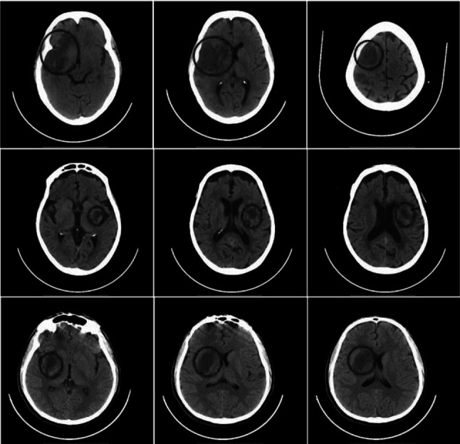
Clinical validation dataset showing ischemic stroke lesion region circled
Methods
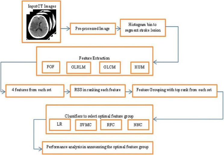
In this research work to segment the ischemic stroke lesion a fully computer aided approach is followed and finding the features in classifying the normal (NR) and abnormal regions (AR). The skull portion is removed from the input CT image using skull stripping algorithm (SSA). Then the proposed histogram bin approach is used to segment the ischemic stroke lesion region. 4 features from each of the four feature sets are extracted, announcing a total of 16 features. 24 Feature Groups (FG) are framed with top ranking features in each group. Finally, four classifiers are introduced to select the best feature group. The methodology followed in this work is presented in the flowchart shown in Fig. 2.
Fig. 2.
Flowchart showing the methodology
Skull stripping algorithm (SSA)
As an initial step, skull stripping need to be done for further processing. The entire process is done in the tissue region only. Hence the removal of skull region has to be done from the input CT image presented in Fig. 3a. To split out the brain and the skull portion, the space occupied by both has to be noted. The connected component method is applied to form a binary mask. On applying this mask over the input CT image, the largely connected tissue portion of the brain region is retained by removing the skull portion as shown in Fig. 3b.
Fig. 3.
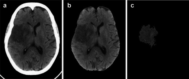
a Input CT image, b Skull stripped image c Segmented ischemic stroke lesion
Proposed histogram bin based novel algorithm (HBBNA) in segmentation
Pearson [27] introduced histogram as probability distribution estimation for a quantifiable variable. The histogram is an efficient statistical approach to get the graphical probability distribution of the given image. Given data can be grouped into sets called bins and bin width defines the number of pixels it can hold. Frequency of occurrence of each pixel in an image represented graphically is histogram. Following are the steps involved to segment the abnormal ischemic stroke region using histogram bin based segmentation approach.
Step 1 To segment the ischemic stroke lesion region, the given input skull stripped CT image (Iinput) intensity values (IV) are grouped into histogram bins (B) as shown in Eq. 1.
| 1 |
where k = 1, 2, 3, 4,…, n. n is the number of bins, k is the bin number.
Step 2 The ischemic stroke lesion region is highly segmentable only when the histogram bins selected is 30. Hence value selected for n is 30. The intensity values of the skull exposed image (Iinput) are grouped into 30 histogram bins [B30(1), B30(2), B30(3), B30(4) …, B30(30)] with a bin width of 8 approximately. Equation 2 narrates the image intensity values after the formation of 30 histogram bins.
| 2 |
where k = 1, 2, 3, 4, …,30.
Step 3 The frequency of occurrence of every intensity values in each bin is recorded. B30(1) represents first bin’s intensity values count (IC) given in Eq. 3. Similarly for 30th bin given in Eq. 4.
| 3 |
| 4 |
Step 4 Sort B30(k)in descending order. Equation 5 gives sorted B30(k) in descendent order (Bsort).
| 5 |
Step 5 The absolute difference between the successive bin values of Bsort(k) are calculated and is given (Bad) in Eq. 6.
| 6 |
where j = 1, 2, 3, 4,…,29.
Step 6 Leave the first highest value (Bad1) because that is the highest value obtained due to the highest count of pixel value 0. This first highest is no way related to lesion segmentation. Leaving the first highest value, Eq. 7 shows the second highest value (Bad2) of Bad which is considered for segmentation.
| 7 |
On average, the Bds2 is the value found when considering the absolute difference between bin 5 and bin 6 of Bsort(k). Bin 6 is effective in lesion segmentation on comparison with bin 5, when a total of 30 bins considered. Hence 6th bin of Bsort(k) can be used for further processing of segmentation.
Step 7 Search for the value Bsort(6) in B30(k). Call Bs to find the bin conforming to Bsort(6) is represented in Eq. 8.
| 8 |
Step 8 Bin analogous to Bs is the optimal bin Bopt to locate the stroke lesion and is given in Eq. 9.
| 9 |
.
Step 9 Bopt, Bopt−1 and Bopt−2 are the bins selected for ischemic stroke lesion segmentation. Bopt−1 and Bopt−2 are the bins preceding Bopt. The region to be segmented is associated with the mentioned three bins and is denoted as Bseg which is given in Eq. 10.
| 10 |
The frequency of occurrence of all intensity values in Bseg makes the IC. Intensity count (ICseg) related to this Bopt, Bopt−1, Bopt−2 are morally liable for ischemic stroke lesion segmentation and is represented in Eq. 11.
| 11 |
Step 10 The intensity values for the considered input CT image ranges from 0 to 255, a total of 256 intensity values. The intensity values (IV) associated to these selected three bins is purely responsible for ischemic stroke lesion region. The segmented ischemic stroke lesion intensity values (IVseg) are given in Eq. 12.
| 12 |
The segmented ischemic stroke lesion section for the given input CT image using this histogram bin approach is presented in Fig. 3c.
The segmented lesion and the ground truth can be compared to declare the validity of the segmented output by any method. As per Akbarzadeh et al. [28] dice similarity coefficient and Jaccard coefficient are the two effective validation metrics to learn about the segmentation results. Interpretation of the obtained coefficients outputs (oco) can be done with the ranges mentioned in this Table 1.
Table 1.
Interpretation using oco range
| S. no. | Range | Interpretation |
|---|---|---|
| 1 | oco<0.2 | Poor agreement |
| 2 | oco between 0.2 and 0.4 | Fair agreement |
| 3 | oco between 0.4 and 0.6 | Moderate agreement |
| 4 | oco between 0.6 and 0.8 | Good agreement |
| 5 | oco between 0.8 and 1 | Excellent agreement |
This HBBNA segmentation method produces dice coefficient of 0.79 and Jaccard coefficient of 0.81 when compared to Shi and Liu [29] work in which their segmentation work produced 0.77 and 0.8.
This novel research work in segmenting ischemic stroke region using histogram bin approach can be compared with Sivakumar and Ganeshkumar [5] work. They proposed brain stroke segmentation method with accuracy of 99.6% when compared to this HBBNA proposed work with accuracy of 99.75%.
Features and classification
Feature extraction
To characterize the properties of the image, significant attributes need to be identified and analyzed. These significant attributes are labeled as features. Most related information in the images is identified and analyzed in the name of features. 16 features for both NR and AR are extracted as 4 features from each feature set.
First order features (FOF)
FOF of an image is better described by the probability distribution of each intensity value. Characterization of the histogram of an image includes various parameters like mean (ME), standard deviation (SD), coarseness index (CI) and skewness (SK) [25].
Gray level run length matrix features (GLRLM)
GLRLM for a specified direction for each element (c, d) is the number of runs with intensity values holding gray level ‘c’ and run length ‘d’. As per Hinzpeter et al. [30] GLRLM features such as short run emphasis (SRE), run percentage (RP), run length nonuniformity (RLN) and low gray level run emphasis (LGRE) are extracted for both NR and AR.
Gray level co-occurrence matrix features (GLCM)
GLCM texture feature computes the relationship between pixel pairs in the images. GLCM features like contrast (CONT), cluster prominence (CP), cluster shade (CS) and sum variance (SV) are extracted for both NR and AR [31]. These listed four features are calculated using the co-occurrence matrix.
Hu’s moment features (HUM)
Moment invariants are widely used as features for image classification. These values are invariant in accordance to translation, scale and rotation [32]. Hu’s moment features like Humoment1 (HuM1), Humoment3 (HuM3), Humoment4 (HuM4) and Humoment6 (HuM6) are extracted for both NR and AR.
The extracted features are tabulated in Table 2.
Table 2.
Features extracted (shown here for 5 CT slices)
| Feature | Region | Image1 | Image2 | Image3 | Image4 | Image5 |
|---|---|---|---|---|---|---|
| ME | NR | 0.46 | 0.46 | 0.46 | 0.41 | 0.43 |
| AR | 0.33 | 0.33 | 0.33 | 0.34 | 0.34 | |
| SD | NR | 0.06 | 0.04 | 0.05 | 0.11 | 0.04 |
| AR | 0.03 | 0.03 | 0.03 | 0.03 | 0.02 | |
| CI | NR | 0.0043 | 0.0024 | 0.0035 | 0.0135 | 0.0024 |
| AR | 0.0009 | 0.0009 | 0.0009 | 0.0011 | 0.0007 | |
| SK | NR | 9.02 | 5.47 | 9.22 | 3.45 | 3.38 |
| AR | 2.86 | 3.86 | 2.92 | 3.18 | 3.04 | |
| SRE | NR | 0.35 | 0.39 | 0.36 | 0.39 | 0.31 |
| AR | 0.45 | 0.40 | 0.43 | 0.45 | 0.34 | |
| RP | NR | 0.10 | 0.09 | 0.09 | 0.16 | 0.05 |
| AR | 0.12 | 0.09 | 0.11 | 0.20 | 0.06 | |
| RLN | NR | 1464.4 | 1670.9 | 1514.6 | 2792.2 | 692.36 |
| AR | 2796.4 | 1740.5 | 2316.4 | 4408.1 | 911.3 | |
| LRGE | NR | 83.24 | 121.2 | 95.14 | 76.39 | 95.70 |
| AR | 136.77 | 98.02 | 122.33 | 125.02 | 117.46 | |
| CONT | NR | 0.08 | 0.08 | 0.07 | 0.12 | 0.05 |
| AR | 0.04 | 0.04 | 0.03 | 0.09 | 0.02 | |
| CP | NR | 78.05 | 61.70 | 77.45 | 98.51 | 36.68 |
| AR | 12.75 | 11.53 | 13.80 | 23.65 | 8.25 | |
| CS | NR | 12.10 | 9.66 | 12.04 | 15.54 | 5.85 |
| AR | 3.16 | 2.76 | 3.32 | 5.59 | 1.90 | |
| SV | NR | 6.19 | 5.69 | 6.20 | 6.94 | 4.97 |
| AR | 4.65 | 4.49 | 4.70 | 5.41 | 4.27 | |
| HuM1 | NR | 0.58 | 0.40 | 0.37 | 0.44 | 0.45 |
| AR | 0.82 | 0.56 | 0.52 | 0.62 | 0.59 | |
| HuM3 | NR | 0.0242 | 0.0018 | 0.0016 | 0.00006 | 0.0080 |
| AR | 0.0759 | 0.0067 | 0.0048 | 0.01972 | 0.0212 | |
| HuM4 | NR | 0.15 | 0.05 | 0.04 | 0.08 | 0.04 |
| AR | 0.31 | 0.10 | 0.08 | 0.17 | 0.09 | |
| HuM6 | NR | 0.0002 | 0.0001 | 0.00002 | 0.0001 | 0.0006 |
| AR | 0.0025 | 0.0002 | 0.00013 | 0.0005 | 0.0029 |
Feature selection by ranking approach
The FOF, GLRLM, GLCM and HUM features are extracted and subjected to statistical analysis to identify the optimal features for classification. To list the optimal features, the analysis of variance (ANOVA) is conducted on each extracted features. The RSS measured for each feature are tabulated. The RSS can be ranked by arranging it in ascending order. The feature with minimum RSS is given rank one and vice versa. From Table 3, features with a minimum rank from each group can be used for classification. So, features within 10 ranks are selected for FG and the selected features are ME, SD, CI, SRE, LGRE, CONT, CP, CS, SV, and HuM4. Initially, it was decided to take four features, one from each group to make the feature group. But since, the first feature group contains the first three ranks, it was later improvised to include an extra feature from the first group to make a feature group with five features. This was done to obtain better output.
Table 3.
Ranking the extracted features
| S. no. | Feature | RSS | Rank |
|---|---|---|---|
| 1 | ME | 6.53 | 1 |
| 2 | SD | 8.15 | 2 |
| 3 | CI | 9.60 | 3 |
| 4 | SK | 11.78 | 14 |
| 5 | SRE | 10.19 | 4 |
| 6 | RP | 12.58 | 16 |
| 7 | RLN | 11.20 | 11 |
| 8 | LRGE | 10.68 | 5 |
| 9 | CONT | 11.10 | 10 |
| 10 | CP | 10.70 | 6 |
| 11 | CS | 10.87 | 7 |
| 12 | SV | 11.00 | 9 |
| 13 | HuM1 | 11.42 | 12 |
| 14 | HuM3 | 11.47 | 13 |
| 15 | HuM4 | 10.88 | 8 |
| 16 | HuM6 | 11.88 | 15 |
In the first feature set, there are 3 features ME, SD, CI which has the highest ranking 1, 2, 3 respectively. Second feature set contains SRE and LRGE with ranking 4, 5 respectively. All features in the third feature set contains ranking within 10. The last feature set contains only one feature HumM4 with rank 8.
The first two columns in the feature group contains features selected from feature set 1 where permutation was used to give input with three possible combinations (1, 2) (2, 3) and (1, 3). The third column contains features from feature group 2 where features ranking 4 and 5 were given to possible combinations of feature set 1. The fourth column contains all features from feature set 3 as all their rankings are within rank 10 hence all the features were considered and was made sure that none of the feature was repeated in the combinations. Since the fourth feature set contains only one feature within ranking 10 (HuM4) it was considered for all feature groups.
Classification
Using the selected 10 features, 24 FGs are framed with 5 features in each group. The classification accuracy (CA) is estimated for each FG using the defined classification algorithms. Maier et al. [33] explained and analyzed nine different classification methods and compared each other using ischemic stroke patient dataset. After analysis, conclusion indicated random decision forest classifier and convolutional neural network classifier outperformed well and provided best segmentation results. To find the optimal feature group, four classifiers are subjected namely logistic regression (LR), support vector machine classifier (SVMC), random forest classifier (RFC) and neural network classifier (NNC).
Logistic regression (LR)
Logistic regression is utilized to describe data and to elucidate the association between one categorical dependent binary variable and one or more independent variables. It is a supervised classification algorithm in which the output takes only the discrete values irrespective of the inputs. This method of classification needs a clear decision threshold. This decision threshold value can be low or high based on the applications. As per categories, it can be classified as binomial, multinomial and ordinal. The performance of this logistic regression can be evaluated using null deviance, model deviance and confusion matrix [34].
Support vector machine classifier (SVMC)
Support vector machines are one of the widely employed machine learning algorithms for classification purposes. It uses supervised learning approach and supports linear classification. A specialty behind this SVM is in maximizing the geometric approach and in minimizing the empirical classification error. Hence it is called as maximum margin classifier and works based on structural risk minimization. A hyper plane is the one which distinguishes between a set of objects having different class memberships. It uses maximal separating hyperplane in which the input vector map to a higher dimensional space. This hyperplane which separates the two hyperplanes on either sides, must be planned in such a way that the distance between these should be high, so that better the generalization error will be. Kernel is the important hyperparameter of SVM and it can be linear, polynomial and radial. The performance of this classifier is highly dependent on the kernel selection and their associated hyperparameters. Radial Basis Function (RBF) kernel is the most widely used, due to its flexibility in separating observations. RBF kernel was used in this research for classification [35].
Random forest classifier (RFC)
A random forest classifier basically applies parallel combinations of decision tree classifiers on various sub-samples of the dataset and utilizes averaging operation to enhance the classification accuracy. It is based on supervised machine learning algorithm and uses decision tree as its base classifier. This approach process randomization in two ways as random sampling of data and random sampling of inputs to generate base classifier. It handles large databases without any input variable deletion, estimates important variables and generalization error, also effective in estimating the missing data. It is easily parallelized for scalability and efficiency [36].
Neural network classifier (NNC)
An artificial neural network classifier architecture is built with numerous artificial neurons which are linked together. The main aim of this architecture is to convert the inputs into significant outputs. Neural networks learn in the presence of noise and the teaching mode can either be supervised or unsupervised. This network comprises of units, prearranged in layers. Every unit, upon applying a processing on the input, creates output to pass it to the next layer. Basically, it comprises of three important layers namely, input layer, hidden layer and output layer. Nodes in each layer connects these layers and the lines that connects these nodes acts as information teller. The challenge hidden in selecting this classifier is associated in grouping of training, learning and transfer function for classification with growing number of features [37].
The performance analysis parameters such as sensitivity, specificity and accuracy are calculated considering all the four classifiers for all the 24 FGs given in Eqs. 13–15. Table 4 shows the confusion matrix to find the performance measures.
| 13 |
| 14 |
| 15 |
Table 4.
Confusion matrix table
| Dataset | Normal (outcome) | Abnormal (outcome) |
|---|---|---|
| Normal (condition) | TN | FP (Type I errors) |
| Abnormal (condition) | FN (Type II errors) | TP |
True negative (TN) is the number of normal region found as normal. True positive (TP) is the number of abnormal regions found as abnormal. False positive (FP) is the number of normal region found as abnormal. False negative (FN) is the number of abnormal regions found as normal. In classification, the normal and abnormal dataset has to be classified correctly. Two cases can be defined for misclassification such as Type I error: If any normal dataset classified wrongly as abnormal region, then it is a positive error. FP and Type II error: If any abnormal dataset classified wrongly as normal region, then it is a negative error, FN. For the 24 FGs, the measured CA using this LR, SVMC, RFC and NNC are tabulated in Table 5.
Table 5.
Classification accuracy of the feature groups for the various classifiers
| Feature group | Feature combination | CA% | |||
|---|---|---|---|---|---|
| LR | SVMC | RFC | NNC | ||
| FG1 | ME, SD, SRE, CP, HuM4 | 86.44 | 93.26 | 87.58 | 93.83 |
| FG2 | ME, SD, SRE, CS, HuM4 | 86.44 | 93.26 | 87.58 | 99.73 |
| FG3 | ME, SD, SRE, SV, HuM4 | 86.44 | 97.8 | 93.91 | 93.91 |
| FG4 | ME, SD, SRE, CONT, HuM4 | 88.71 | 95.53 | 93.91 | 99.73 |
| FG5 | SD, CI, SRE, CP, HuM4 | 68.26 | 84.17 | 93.91 | 93.91 |
| FG6 | SD, CI, SRE, CS, HuM4 | 70.53 | 84.17 | 75.08 | 87.58 |
| FG7 | SD, CI, SRE, SV, HuM4 | 68.26 | 86.44 | 93.91 | 99.73 |
| FG8 | SD, CI, SRE, CONT, HuM4 | 70.53 | 93.26 | 87.58 | 87.58 |
| FG9 | ME, CI, SRE, CP, HuM4 | 86.44 | 97.8 | 93.91 | 93.91 |
| FG10 | ME, CI, SRE, CS, HuM4 | 86.44 | 97.8 | 93.91 | 87.58 |
| FG11 | ME, CI, SRE, SV, HuM4 | 86.44 | 97.8 | 87.58 | 93.91 |
| FG12 | ME, CI, SRE, CONT, HuM4 | 88.71 | 97.8 | 99.73 | 99.73 |
| FG13 | ME, SD, LGRE, CP, HuM4 | 84.17 | 90.98 | 93.91 | 99.73 |
| FG14 | ME, SD, LGRE, CS, HuM4 | 84.17 | 90.98 | 99.73 | 99.73 |
| FG15 | ME, SD, LGRE, SV, HuM4 | 84.17 | 90.98 | 99.73 | 99.73 |
| FG16 | ME, SD, LGRE, CONT, HuM4 | 84.17 | 90.98 | 99.73 | 87.58 |
| FG17 | SD, CI, LGRE, CP, HuM4 | 72.80 | 84.17 | 93.91 | 87.58 |
| FG18 | SD, CI, LGRE, CS, HuM4 | 72.80 | 86.44 | 87.58 | 93.91 |
| FG19 | SD, CI, LGRE, SV, HuM4 | 72.80 | 86.44 | 81.33 | 87.58 |
| FG20 | SD, CI, LGRE, CONT, HuM4 | 72.80 | 86.44 | 81.33 | 93.91 |
| FG21 | ME, CI, LGRE, CP, HuM4 | 81.89 | 88.71 | 93.91 | 93.91 |
| FG22 | ME, CI, LGRE, CS, HuM4 | 81.89 | 88.71 | 93.91 | 81.33 |
| FG23 | ME, CI, LGRE, SV, HuM4 | 81.89 | 88.71 | 93.91 | 99.73 |
| FG24 | ME, CI, LGRE, CONT, HuM4 | 84.17 | 88.71 | 93.91 | 99.73 |
Those combination yielded significant results. Hence to highlight, it was given in bold font
Results and discussions
This novel work is instigated on Intel(R) Core(TM) i3-3110 M CPU, 2.40 GHZ, ×64-based processor with 4 GB RAM using MATLAB 15. The FG with maximum sensitivity is selected as the optimal FG in classifying the normal and abnormal ischemic stroke lesion regions. As per centum sensitivity approach, FGs from 1 to 24 under LR, FGs 4, 9, 10, 11, 12, 13, 14, 15, 16, 17, 18, 19, 20, 21, 22, 23 and 24 under SVMC, FGs 2, 3, 4, 5, 7, 11, 12, 13, 14, 15, 16, 18, 21, 22, 23 and 24 under RFC and FGs 4, 11, 12, 13, 14, 15, 16 and 24 under NNC are selected as the perfect FGs in classification. On analysis FGs with maximum sensitivity by all the four classifiers are FGs 4, 11, 12, 13, 14, 15, 16, 24. Hence, these eight FGs are known to be the leading FGs accepted by the defined classifiers. It could be noted that, though the FGs 2, 4, 7, 12, 13, 14, 15, 16, 23 and 24 possess 99.73% CA in any one of the classifier, it is accepted as an optimal FG only if it yields maximum sensitivity. Hence, the FG’s 4, 11, 12, 13, 14, 15, 16, 24 are identified as the FG’s with the optimal set of features presented in bolded letters in Table 5. These selected 8 FGs are validated using fourfold cross validation and their obtained CA’s are plotted and tabulated correspondingly. When comparing the CA’s of FG’s, the FG12 reports maximum CA with referred to all the four classification algorithms namely LR, SVMC, RFC and NNC.
From Figs. 4, 5, 6 and 7, the optimal FG to differentiate the NR and AR is FG12, which includes ME, CI, SRE, CONT and HuM4 as its feature combination. ME and CI features from FOF, SRE feature from GLRLM, CONT feature from GLCM and HuM4 feature from HUM as a combination produces the optimum CA.
Fig. 4.
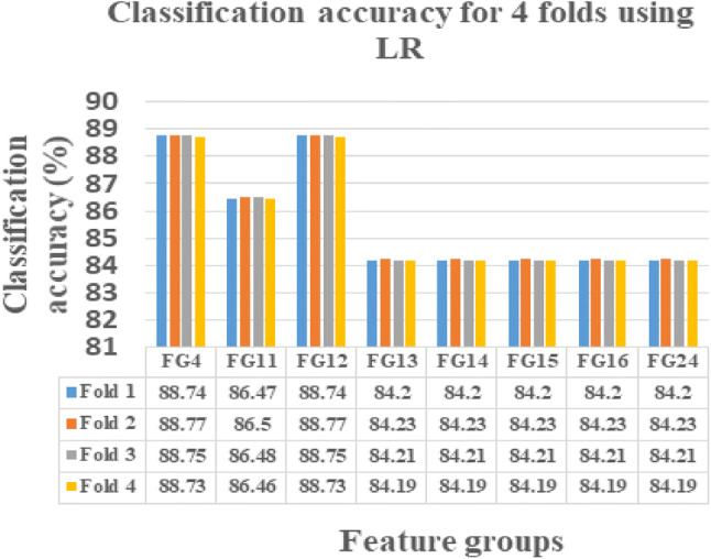
LR showing CA’s of selected 8 FG’s for fourfolds
Fig. 5.
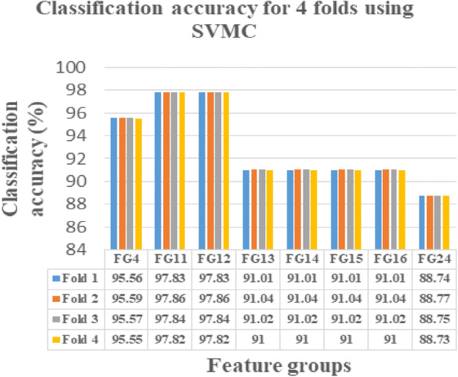
SVMC showing CA’s of selected 8 FG’s for fourfolds
Fig. 6.
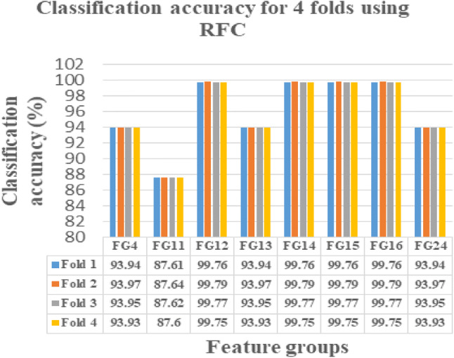
RFC showing CA’s of selected 8 FG’s for fourfolds
Fig. 7.
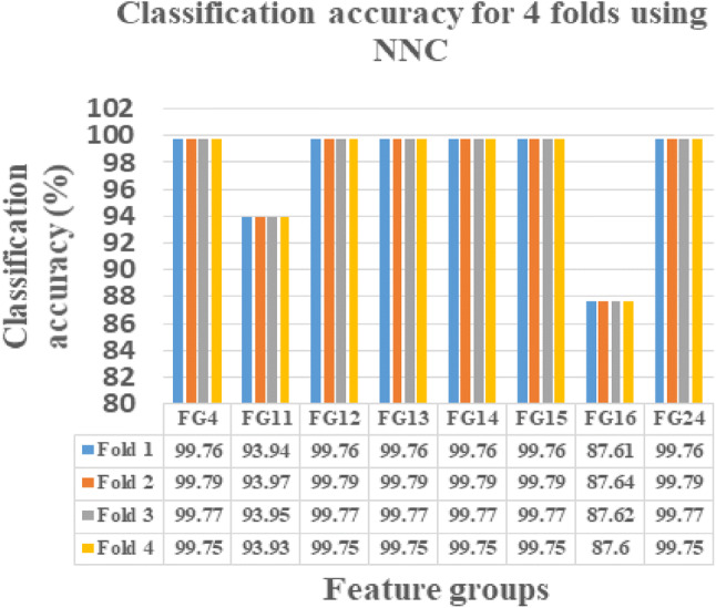
NNC showing CA’s of selected 8 FG’s for fourfolds
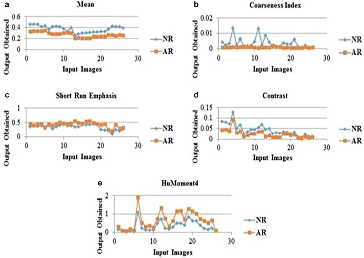
Hence, as per Table 5, on considering the first position based on CA and statistical analysis of FG12, 5 features such as ME, CI, SRE, CONT and HuM4 are selected as the prime features in classifying the NR and AR. Hence of the 16 features extracted, FG12 feature combination is the crucial combination with maximum CA in classifying the NR and AR. Figure 8 presents the selected features showing plots in differentiating NR and AR.
Fig. 8.
Normal and abnormal ischemic stroke lesion region differentiation plot using a mean feature, b coarseness index feature, c short run emphasis feature, d contrast feature, e Humoment4 feature
This novel research work in segmenting ischemic stroke region using histogram bin and optimal features selection approach can be compared with the other existing methodologies by Chawla et al. [14], Tyan et al. [21], Hema Rajini and Bhavani [20], Hajimani et al. [31], and Subudhi et al. [7], based on the performance measures. Chawla et al. [14], proposed automatic detection and classification with a three step approach producing CA about 90%. Tyan et al. [21], proposed a computer aided diagnostic system using four step unsupervised feature perception resulting in CA of 85.55%. Hema Rajini and Bhavani [20], proposed a five stage computer aided approach to segment and analyze ischemic stroke results with a CA of 98%, 97%, 96% and 92% using SVM, k-NN, ANN and decision tree respectively. Hajimani et al. [31], proposed radial basis function neural network (RBFNN) based automated stroke identification system producing 94.4% CA. Subudhi et al. [7] proposed expectation-maximization algorithm for ischemic stroke lesion segmentation and produced 93.4% CA using RF classifier.
In the above mentioned proposed methods of various authors in finding lesion and accuracy measurement, the features are not grouped. The novelty introduced in this article, segments ischemic stroke and after feature ranking, features are grouped to find which group shows maximum accuracy when subjected to any classifier. FG12 produces the better accuracies as 88.77%, 97.86%, 99.79% and 99.79%, by LR, SVMC, RFC and NNC. The uniqueness in this work can be highlighted in such a way that feature not applied as a single to any classifier, instead as group in producing a maximum classification accuracy.
Conclusion
This research work provides a computer assisted histogram bin based segmentation approach to identify the ischemic stroke lesion in brain CT images. After segmenting the stroke lesion, the property of the segmented region is studied with the help of the features. Following to segmentation, the other approaches concluding this article are, optimal feature selection, feature grouping, performance analysis of each group using classifiers and finding the best FG. Every FG is subjected to find the performance analysis using the mentioned classifiers. With maximum sensitivity approach, the optimal 8 FGs are selected out of 24 FGs. After applying fourfold cross validation over these selected FGs, if we compare the CA’s of all FG, FG12 combo reports maximum CA with referred to all the four classification algorithms. ME and CI from FOF, SRE from GLRLM, CONT from GLCM and HuM4 from HUM forms the FG12. This FG12 with optimal features holds the CA of 88.77%, 97.86%, 99.79% and 99.79%, which has been obtained by LR, SVMC, RFC and NNC. Hence this novel approach detects and segments the ischemic stroke lesion region and finds the most distinguishing features in classifying the NR and AR. This work can be extended with more number of datasets to identify other types of stroke lesions.
Compliance with ethical standards
Conflict of interest
The authors declare that they have no conflict of interests.
Ethical approval
This article does not contain any studies with animals performed by any of the authors.
Footnotes
Publisher's Note
Springer Nature remains neutral with regard to jurisdictional claims in published maps and institutional affiliations.
References
- 1.Xiao-Ying Y, Li-Qiong W, Jin-Gen L, Ning L, Ying W, Jian-Ping L. Chinese herbal medicine Dengzhan–Shengmai capsule as adjunctive treatment for ischemic stroke: a systematic review and meta-analysis of randomized clinical trials. Complement Ther Med. 2017 doi: 10.1016/j.ctim.2017.12.004. [DOI] [PubMed] [Google Scholar]
- 2.Paramasivam S. Current trends in the management of acute ischemic stroke. Neurol India. 2015;63:665–672. doi: 10.4103/0028-3886.166547. [DOI] [PubMed] [Google Scholar]
- 3.Karthik R, Menaka R. A critical appraisal on wavelet based features from brain MR images for efficient characterization of ischemic stroke injuries. Electron Lett Comput Vis Image Anal. 2016;15(3):1–16. [Google Scholar]
- 4.Karthik R, Menaka R. Computer-aided detection and characterization of stroke lesion—a short review on the current state-of-the art methods. Imaging Sci J. 2018;66(1):1–22. [Google Scholar]
- 5.Sivakumar P, Ganeshkumar P. An efficient automated methodology for detecting and segmenting the ischemic stroke in brain MRI images. Int J Imaging Syst Technol. 2017;27:265–272. [Google Scholar]
- 6.Clèrigues A, Valverde S, Bernal J, Freixenet J, Oliver A. Xavier Lladó Acute ischemic stroke lesion core segmentation in CT perfusion images using fully convolutional neural networks. Comput Biol Med. 2019;115:103487. doi: 10.1016/j.compbiomed.2019.103487. [DOI] [PubMed] [Google Scholar]
- 7.Subudhi A, Dash M, Sabut S. Automated segmentation and classification of brain stroke using expectation-maximization and random forest classifier. Biocybern Biomed Eng. 2019;40:277–289. [Google Scholar]
- 8.Dreyer R, Murugiah K, Nuti SV, Dharmarajan K, Chen SI, Chen R, Wayda B, Ranasinghe I. Most important outcomes research papers on stroke and transient ischemic attack. Dallas: American Heart Association Inc; 2014. pp. 191–204. [DOI] [PubMed] [Google Scholar]
- 9.Ahmadi A, Khaledifar A, Etemad K. Risk factors associated with hospital mortality in myocardial infarction patients, with and without stroke: a national study in Iran. J Res Med Sci. 2016;21:74. doi: 10.4103/1735-1995.189687. [DOI] [PMC free article] [PubMed] [Google Scholar]
- 10.Davisa A, Gordillob N, Montsenya E, Aymericha FX, López-Córdovad M, Mejiab J, Ortegab L, Mederose B. Automated detection of parenchymal changes of ischemic stroke innon-contrast computer tomography: a fuzzy approach. Biomed Signal Process Control. 2018;45:117–127. [Google Scholar]
- 11.Karthik R, Gupta U, Ashish Jha R, Rajalakshmi R Menaka. A deep supervised approach for ischemic lesion segmentation from multimodal MRI using Fully Convolutional Network. Appl Soft Comput J. 2019;84:105685. [Google Scholar]
- 12.YinshengGuo Yue Ma, Zhang Y, Zhou L, Huang S, Wen Y, FeiZou JC. Autophagy-related gene microarray and bioinformatics analysis for ischemic stroke detection. Biochem Biophys Res Commun. 2017;489:48–55. doi: 10.1016/j.bbrc.2017.05.099. [DOI] [PubMed] [Google Scholar]
- 13.Wu P, Zhou YM, Zeng F, Li ZJ, Luo L, Li YX, Fan W, Qiu LH, Qin W, Chen L, Bai L, Nie J, Zhang S, Xiong Y, Bai Y, Yin CX, Liang FR. Regional brain structural abnormality in ischemic stroke patients: a voxel-based morphometry study. Neural Regen Res. 2016;11(9):1424–1430. doi: 10.4103/1673-5374.191215. [DOI] [PMC free article] [PubMed] [Google Scholar]
- 14.Chawla M, Sharma S, Sivaswamy J, Kishore L 2009. A method for automatic detection and classification of stroke from brain CT images. In: Proceedings of the annual international conference on engineering in medicine and biology society. 2009; 3581–84. [DOI] [PubMed]
- 15.Karthik R, Menaka R. A multi-scale approach for detection of ischemic stroke from brain MR images using discrete curvelet transformation. Elseiver, Measurement. 2017;100:223–232. [Google Scholar]
- 16.Wand MP. Data-Based Choice of Histogram Bin Width. 1997;51(1):59–64. [Google Scholar]
- 17.Weiming H, Xie N, Ruiguang H, Ling H, Chen Q, Yan S, Maybank S. Bin ratio-based histogram distances and their application to image classification. IEEE Trans Pattern Anal Mach Intell. 2014;36(12):2338–2352. doi: 10.1109/TPAMI.2014.2327975. [DOI] [PubMed] [Google Scholar]
- 18.Liu H-S, Chiang S-W, Chung H-W, Tsai P-H, Hsu F-T, Cho Nai-Yu, Wang C-Y, Chou M-C, Chen Cheng-Yu. Histogram Analysis of T2_-Based Pharmacokinetic Imaging in Cerebral Glioma Grading. Comput Methods Programs Biomed. 2017 doi: 10.1016/j.cmpb.2017.11.011. [DOI] [PubMed] [Google Scholar]
- 19.Srikanth B, Padmaja G, Hima Bindu M. An automatic diagnostic system for CT brain image classification. Int J Eng Res Technol (IJERT). 2012;1.
- 20.Hema Rajini N, Bhavani R. Computer aided detection of ischemic stroke using segmentation and texture features. Measurement. 2013;46:1865–1874. [Google Scholar]
- 21.Tyan Y-S, Wu M-C, Chin C-L, Kuo Y-L, Lee M-S, Chang H-Y. Ischemic stroke detection system with a computer-aided diagnostic ability using an unsupervised feature perception enhancement method. Int J Biomed Imaging. 2014;2014(2014):1–12. doi: 10.1155/2014/947539. [DOI] [PMC free article] [PubMed] [Google Scholar]
- 22.Gillebert CR, Humphreys GW, Mantini D. Automated delineation of stroke lesions using brain CT images. NeuroImage Clin. 2014;4:540–548. doi: 10.1016/j.nicl.2014.03.009. [DOI] [PMC free article] [PubMed] [Google Scholar]
- 23.Ray A, Bandyopadhyay SK. Automatic detection of ischemic stroke lesion using textural analysis from brain ct images. Eur J Biomed Pharm Sci. 2016;3(10):282–288. [Google Scholar]
- 24.Li Y, Ng DKS, Kwok JMY 2016. Computer aided detection method for ischemic stroke using feature based approach. Int J Eng Res Sci 2016; 2(10).
- 25.Kanchana R, Menaka R. A novel approach for characterization of ischaemic stroke lesion using histogram bin-based segmentation and gray level co-occurrence matrix features. The Imaging Science Journal. 2017 [Google Scholar]
- 26.Lo C-M, Hung P-H, Hsieh KL-C. Computer-aided detection of hyperacute stroke based on relative radiomic patterns in computed tomography. Appl Sci MDPI. 2019;2019;9(8):1668. [Google Scholar]
- 27.Pearson K. Contributions to the mathematical theory of evolution-II. Skew variation in homogeneous material. Philos Trans R Soc A. 1985;186:343–425. [Google Scholar]
- 28.Akbarzadeh A, Gutierrez D, Baskin A, Ay MR, Ahmadian A, Riahi Alam N, Lövblad KO, Zaidi H. Evaluation of whole-body MR to CT deformable image registration. J Appl Clin Med Phys. 2013 doi: 10.1120/jacmp.v14i4.4163. [DOI] [PMC free article] [PubMed] [Google Scholar]
- 29.Shi W, Liu H 2019. Modified U-net architecture for ischemic stroke lesion segmentation and detection. In: 2019 IEEE 4th advanced information technology, electronic and automation control conference (IAEAC 2019).
- 30.Hinzpeter R, Wagner MW, Wurnig MC, Seifert B, Manka R, Alkadhi H. Texture analysis of acute myocardial infarction with CT: first experience study. PLoS ONE. 2017;12(11):e0186876. doi: 10.1371/journal.pone.0186876. [DOI] [PMC free article] [PubMed] [Google Scholar]
- 31.Hajimani E, Ruano MG, Ruano AE. An intelligent support system for automatic detection of cerebral vascular accidents from brain CT images. Comput Methods Programs Biomed. 2017;146:109–123. doi: 10.1016/j.cmpb.2017.05.005. [DOI] [PubMed] [Google Scholar]
- 32.Reboucüas Filho PP, Moura Sarmento R, Bandeira Holanda G, de Alencar LD. New approach to detect and classify stroke in skull CT images via analysis of brain tissue densities. Comput Methods Programs Biomed. 2017 doi: 10.1016/j.cmpb.2017.06.011. [DOI] [PubMed] [Google Scholar]
- 33.Maier O, Schröder C, Forkert ND, Martinetz T, Handels H. Classifiers for ischemic stroke lesion segmentation: a comparison study. PLoS ONE. 2015;10(12):e0145118. doi: 10.1371/journal.pone.0145118. [DOI] [PMC free article] [PubMed] [Google Scholar]
- 34.Dinh TA, Silander T, Tchoyoson Lim CC, Leong T-Y. An automated pathological class level annotation system for volumetric brain images. AMIA Annu Symp Proc. 2012;2012(2012):1201–1210. [PMC free article] [PubMed] [Google Scholar]
- 35.Magi SM, Elemmi M, Shirol V. Classification of human brain strokes using CT images. J Image Process Artif Intell. 2016;2(2):1–11. [Google Scholar]
- 36.Paul D, Ruan S. ModzelewskiRomain, VauclinSebastien, Vera Pierre, Gardin Isabelle. Feature selection for outcome prediction in oesophageal cancer using genetic algorithm and random forest classifier. 2016 doi: 10.1016/j.compmedimag.2016.12.002. [DOI] [PubMed] [Google Scholar]
- 37.Sharma H, Zerbe N, Klempert I, Hellwich O, Hufnagl P. Deep convolutional neural networks for automatic classification of gastric carcinoma using whole slide images in digital histopathology. Comput Med Imaging Graphics. 2017;2017(61):2–13. doi: 10.1016/j.compmedimag.2017.06.001. [DOI] [PubMed] [Google Scholar]


