Sampling Performance of Multiple Independent Molecular Dynamics Simulations of an RNA Aptamer

Abstract

Using multiple independent simulations instead of one long simulation has been shown to improve the sampling performance attained with the molecular dynamics (MD) simulation method. However, it is generally not known how long each independent simulation should be, how many independent simulations should be used, or to what extent either of these factors affects the overall sampling performance achieved for a given system. The goal of the present study was to assess the sampling performance of multiple independent MD simulations, where each independent simulation begins from a different initial molecular conformation. For this purpose, we used an RNA aptamer that is 25 nucleotides long as a case study. The initial conformations of the aptamer are derived from six de novo predicted 3D structures. Each of the six de novo predicted structures is energy minimized in solution and equilibrated with MD simulations at high temperature. Ten conformations from these six high-temperature equilibration runs are selected as initial conformations for further simulations at ambient temperature. In total, we conducted 60 independent MD simulations, each with a duration of 100 ns, to study the conformation and dynamics of the aptamer. For each group of 10 independent simulations that originated from a particular de novo predicted structure, we evaluated the potential energy distribution of the RNA and used recurrence quantification analysis to examine the sampling of RNA conformational transitions. To assess the impact of starting from different de novo predicted structures, we computed the density of structure projection on principal components to compare the regions sampled by the different groups of ten independent simulations. The recurrence rate and dependence of initial conformation among the groups were also compared. We stress the necessity of using different initial configurations as simulation starting points by showing long simulations from different initial structures suffer from being trapped in different states. Finally, we summarized the sampling efficiency for the complete set of 60 independent simulations and determined regions of under-sampling on the potential energy landscape. The results suggest that conducting multiple independent simulations using a diverse set of de novo predicted structures is a promising approach to achieve sufficient sampling. This approach avoids undesirable outcomes, such as the problem of the RNA aptamer being trapped in a local minimum. For others wishing to conduct multiple independent simulations, the analysis protocol presented in this study is a guide for examining overall sampling and determining if more simulations are necessary for sufficient sampling.

Introduction

Aptamers are single-stranded RNA or DNA oligonucleotides that are capable of binding noncovalently to diverse biological targets with high affinities and specificities.¹ In this work, RNA aptamers are studied and the term aptamer will be used to mean “RNA aptamer”. Knowledge of the conformations that an aptamer adopts in solution is crucial to understand the ligand binding functions of the aptamer. Small changes in aptamer conformation can have significant effects on its binding properties, especially in the applications of biosensors.² Hence, it is of great importance to characterize possible aptamer conformations when designing new applications. For example, when optimizing an aptamer for use in a biosensor, one may wish to exploit situations in which an aptamer experiences a large conformational change upon ligand binding. However, the number of available aptamer structures characterized by experimental methods, such as X-ray crystallography, NMR, and cryoelectron microscopy, is considerably limited compared to the number of aptamers being discovered.³ To overcome this challenge, computational methods can assist in providing insights into the conformations of aptamers in solution.

For aptamers with no 3D structure characterized by experiment, computational methods can supplement this gap. Specifically, RNA 3D structure prediction that relies solely on primary sequence or is augmented with biochemical information has been successfully applied to riboswitches.⁴ Such in silico structure prediction permits modeling studies that investigate large conformational changes in aptamers. Studies of this type are important for understanding molecular mechanisms.³⁻⁵ Although in silico structure prediction might be less reliable for larger RNA molecules, for example, the 185-nt ribozyme,⁴ for small molecules such as stem-loops, it is highly reliable. Therefore, the RNA motifs found in aptamers are good candidates for studying the sampling performance of molecular dynamics (MD) simulation.

While RNA 3D structure prediction generates conformations that are stable with respect to energetics, it is necessary to investigate the dynamics of the structures with MD simulations. Classical MD simulation generates a conformational ensemble of RNA structures at equilibrium. MD simulations complement experimental studies by providing detailed atomic motions that aid in understanding the structure–function relationship.^6,7 For aptamers whose 3D structures have not been experimentally solved, a combined effort of RNA 3D structure prediction and MD simulations can effectively render their conformations. MD simulations further refine the predicted structures with an accurate all-atom force field and explore the dynamics of RNA molecules in solvent.

The ideal ensemble obtained from an MD simulation consists of N completely independent and identically distributed configurations. However, an MD simulation generates samples that are correlated. If the simulation is long enough, the ergodic hypothesis is satisfied, that is, the time average obtained from the simulation equals the ensemble average as measured in the experiment. Hence, the limited timescale of an MD simulation leads to a sampling problem.⁸ Equilibrium sampling requires access to all regions of configuration space (or at least to those regions with significant populations) and requires that configurations have the correct relative probabilities.⁸ Efforts have been made in the field to define an independent sample in regard to sampling assessment.^9,10 For example, according to the effective sample size approach developed by Lyman and Zuckerman,⁹ 200 or 250 frames from a 1 μs simulation of a highly flexible pentapeptide metenkephalin were selected. Extending the simulations and conducting multiple independent simulations are possible options to increase the number of independent samples. The approach of using multiple MD runs starting from different initial conditions¹¹ has been proven to be a promising approach to enhance equilibrium sampling.^11,12 It has been concluded that multiple independent short simulations not only sample more broadly in the conformational space compared to a single long trajectory¹³ but also provide more accurate estimates.¹⁴ In this study, the discussion of sampling focuses on the ability to discover as many states as possible, mainly for MD applications in describing the structure and dynamics of a particular state of a biomolecular system (apo or bound state). The transition pathway between states involved in folding and unfolding is not included. Although more complicated sampling schemes, such as adaptive sampling¹⁵ and goal-oriented fluctuation amplification of specific traits algorithm,¹⁶ have been proposed to better target the native state and converge on the Markov state models for pathway, parallel simulations may offer a significant enhancement in the observation of rare events and thoroughly explore the landscape around the starting state.¹⁷

Although the sampling problem is widely recognized in the field of biomolecular simulation, a standard procedure for conducting multiple independent MD simulations and assessing the impact on equilibrium sampling is still yet to be developed, especially for molecules with no experimentally characterized structures available. For example, many investigators report in their studies that simulations were run at least twice to validate the consistency and reproducibility^2,18 and calculate averages^19,20 from the repeated runs to estimate properties. Others have shown that a large number of short MD simulations can be further analyzed via Markov state models to study the transitions of substates.^21,22 However, it is unclear how to determine the length of simulations to run and how to analyze the results from multiple short independent MD simulations. It is suggested that each simulation should be long enough to overcome local barriers that surround the starting point.¹³ Additionally, the simulation length also depends on the number of degrees of freedom and the correlation time for the property of interest under study.⁸ However, it might be difficult to distinguish between kinetic trapping in a basin and convergence because the consequent plateauing of the properties of interest can falsely suggest convergence.²³ Even when an independent simulation is long, it can be trapped at some state during the simulation. Convergence must also be assessed both globally and locally. Specifically, the two expectations of sampling from multiple independent MD simulations are (1) a wide region of the conformational space should be sampled (global) and (2) a partial overlap between different trajectories should be achieved (local).²⁴ To achieve these goals, rigorous quantitative evaluation approaches are crucial to assess the sampling performance.

The focus of this study was to investigate the sampling performance of multiple independent MD simulations from different initial conformations using analysis protocols suited for a nonlinear dynamical system in reduced phase space. In this work, we combined RNA 3D structure prediction with multiple independent MD simulations to study the conformation and dynamics of an RNA aptamer. The initial structures used in the independent MD simulations were selected to achieve diversity in both conformation and energy. We show how each independent simulation samples the RNA potential energy and contributes to the overall potential energy distribution for the aptamer. Upon comparing the RNA potential energy distributions among the groups of simulations from various predicted models, we show that the shapes and peaks of the distributions vary for independent simulations within each group; however, the distributions as compared across groups were consistent. The conformational transitions identified from recurrence quantification analysis (RQA) show the same results among the groups. Using principal component analysis (PCA), it is shown that simulations initiated from different predicted models were able to explore regions that had not been visited by other groups. With support from RQA results, we are able to interpret that there may be barriers in the conformational space for the aptamer that are difficult to overcome. Overall, the 60 independent simulations yield sufficient sampling with no obvious kinetic traps. The undersampled region was also identified from the potential energy landscape, which might provide guidance for future simulations.

The remainder of the paper is organized as follows. The Methods section introduces model selection from 3D prediction and MD simulation details, as well as data analysis approaches. In the Results and Discussion section, the simulation results and analyses are presented. A brief summary and further discussion are given in the Conclusions section.

Results and Discussion

In this section, we describe the results of our multiple independent MD simulations of the NEO2A aptamer. In the discussion, we use the term “configuration” to describe the six different predicted structures and use the term “conformation” to refer to the 10 variations of each predicted structure as starting points of MD simulations. We began by studying how 10 independent simulations, starting from the same configuration help avoid the trajectories being trapped. We can also compare different groups of simulations using different configurations. Because there is no 3D structure available in the Protein Data Bank (PDB) for the NEO2A aptamer, model selection on characterizing the conformation and dynamics of a flexible RNA aptamer is of great importance. We examined the sampling from all the 60 independent simulations and identified possible unsampled regions for future guidance of MD simulations.

Multiple Independent Simulations Started from the Same Predicted Model Help Avoid Local Energy Minima Traps

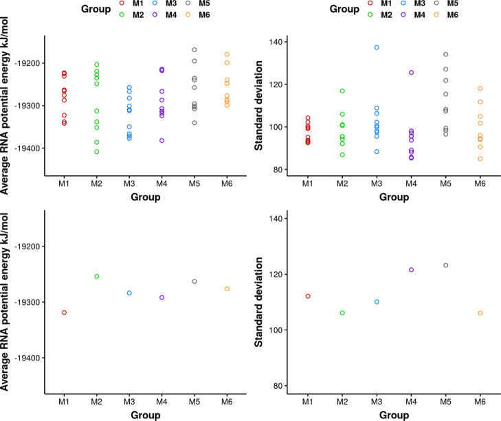
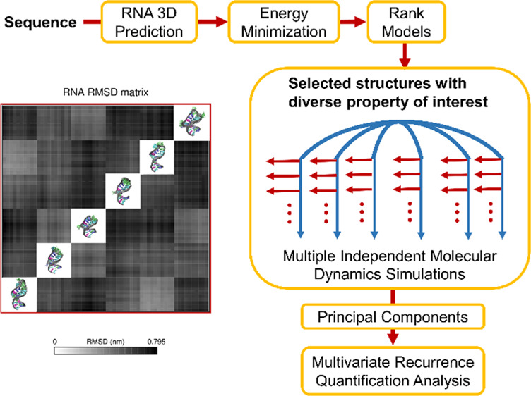
Six configurations were selected from de novo prediction with various potential energy values. From each of these de novo structures, 10 conformations were generated as initial structures for multiple independent MD simulations. Screenshots of the 60 initial structures after structural superimposition are shown in Figure S1. From the root-mean-square deviation (rmsd) matrix in Figure S2, the structures show greater structural similarity within each group generated from the same configuration, while exhibiting larger variations between groups. To examine if the predicted models were better relaxed in 10 independent simulations, the mean and variance of the RNA potential energy were compared among groups of simulations from different predicted models. The expectation is that 10 independent simulations can sample more broadly and recover the correct potential energy distribution, even though the initial structures were selected with variations in potential energy. The mean and standard deviation of the RNA potential energy were calculated. From Figure 1, the spread of average RNA potential energy from different groups shows overlap. It indicates averaging from 10 simulations can improve the estimation accuracy and reduce the bias from each independent simulation. Figure S3 shows the distribution of RNA potential energy in each group, while Figure S4 describes the distribution from each independent simulation within the group. Thus, the distributions from different groups in Figure S3 are expected to be more similar than the distributions from various independent simulations in Figure S4. In Figure S3, the distributions from the whole group adopted a more similar bell shape with peak values around −19,270 kJ/mol. Distinct peaks from independent simulations shown in Figure S4 merged when combining 10 simulations in each group, which reduces the appearance of an obvious bimodal or multimodal shape in any group. For example, simulations S4 and S6 in group M4 exhibit different peak values, while the combination of 10 short simulations in M4 shows no bimodal shape. If only two simulations S4 and S6 were conducted, the results would be biased. Hence, we recommend conducting a large number of simulations instead of two or three simulations, when the simulation length is relatively short. In summary, the predicted models selected for MD simulations are diverse in system potential energy. However, the RNA potential energy from a combination of multiple independent simulations adopted a consistent distribution. These results indicate that using a multiple independent simulations approach with limited timescales helps relax the structure and reduce the possibility of the structure being trapped by a local energy minimum around initial structures. The results indicate that for each configuration, multiple independent simulations are necessary to achieve sufficient sampling.

Figure 1.

Mean (left) and standard deviation (right) of RNA potential energy calculated from each 100 ns simulation (top) and 10 simulations in each group (bottom).

To further test if 10 independent simulations can achieve satisfactory sampling for each group, the standard error of the mean of potential energy was calculated to examine the error generated by 10 simulations (Figure 2). In each group, a different number of independent simulations were randomly selected, and the combinations of these data were used for error calculation. The standard error was then plotted against the number of independent simulations. The diamond symbols represent the error calculated from simulations in each group. As the number of simulations increases, the variations of the standard error in each group decrease. Although the trend of error versus might not be strictly followed in some groups, the trend is clear when taking all the groups together. Together with Figure 1, the results indicate that multiple independent simulations can improve the accuracy of the estimation of a property of interest by decreasing the error of the average. From the plot, 10 independent simulations can achieve good sampling with standard error below 2 kJ/mol of RNA potential energy. Following this method, the standard error of the mean of a property of interest can be used to estimate the number of simulations necessary for satisfactory sampling, given the expected error.

Figure 2.

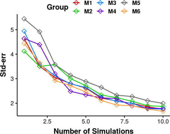
Standard error of the mean of RNA potential energy as a function of the number of simulations in each group. The simulations were randomly chosen from a total of 10 independent simulations in each group.

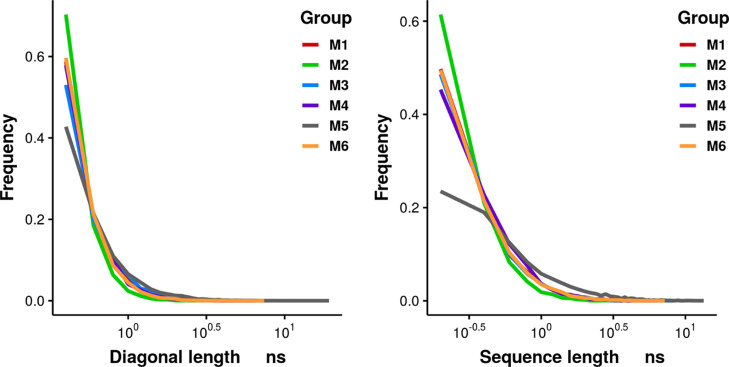
To quantitatively investigate the ability of multiple independent simulations in each group to overcome local energy minima, the serial correlations in the simulations were studied by RQA. The diagonal length (DL) characterizes the average length of sequences, where the structures had similar conformations with structures separated by certain time lags along the trajectory. The DL was calculated at each time lag, and then, the DL distribution was plotted. The sequence length (SL) is defined as the length of vertical sequence from each entry on the main diagonal in the recurrence plot (RP). It measures how long a structure in the simulation can form a subtrajectory with sequential structures that have similar conformations. The frequency of DL in Figure 3 shows that most DLs are below 1 ns, which indicates that a simulation segment shorter than 1 ns is more likely to be correlated with another segment with the same length separated at some lag. It shows that most transitions reflected from the RP of each simulation are in a relatively short timescale compared with the length of simulations (100 ns). It is noticeable that there is a long tail in the distribution of DL, which indicates that the maximum DL can be much larger than most DLs. The sequence on the diagonal in the RP, measured by DL, represents correlated simulation segments separated by some lag. To further investigate how many sequential structures are structurally similar along the trajectory, the frequency of SL is plotted in Figure 3. The groups show similar SL frequency below 1 ns in the distribution of SL except group M5, which exhibits large SLs that do not exist in other groups. It indicates that there is long sub-trajectory with similar structures in group M5 simulations. In summary, the six groups show consistent frequencies of DL with main DLs at values smaller than 1 ns, which indicates that the sequentially correlated structures are well-sampled by having multiple independent simulations in each group. That DL and SL having different values indicates that there exist conformational states with different timescales. It further indicates that the multiple simulations in each group are able to capture these conformational transitions effectively. In summary, finding the recurrent length that reaches relatively low frequency can provide insight into the minimum length of each simulation needed to achieve sufficient sampling of the transitions. Consistent recurrent length frequencies among different groups of multiple short simulations indicates that the sampling in each group is sufficient, which can also be used to adjust the number of simulations within each group for sufficient sampling.

Figure 3.

Frequency of DL (left) and SL (right) from 10 independent short simulations in different groups.

Multiple Sets of Multiple Independent Simulations, from Different Predicted Models, Improve the Sampling Diversity in the Energy Landscape

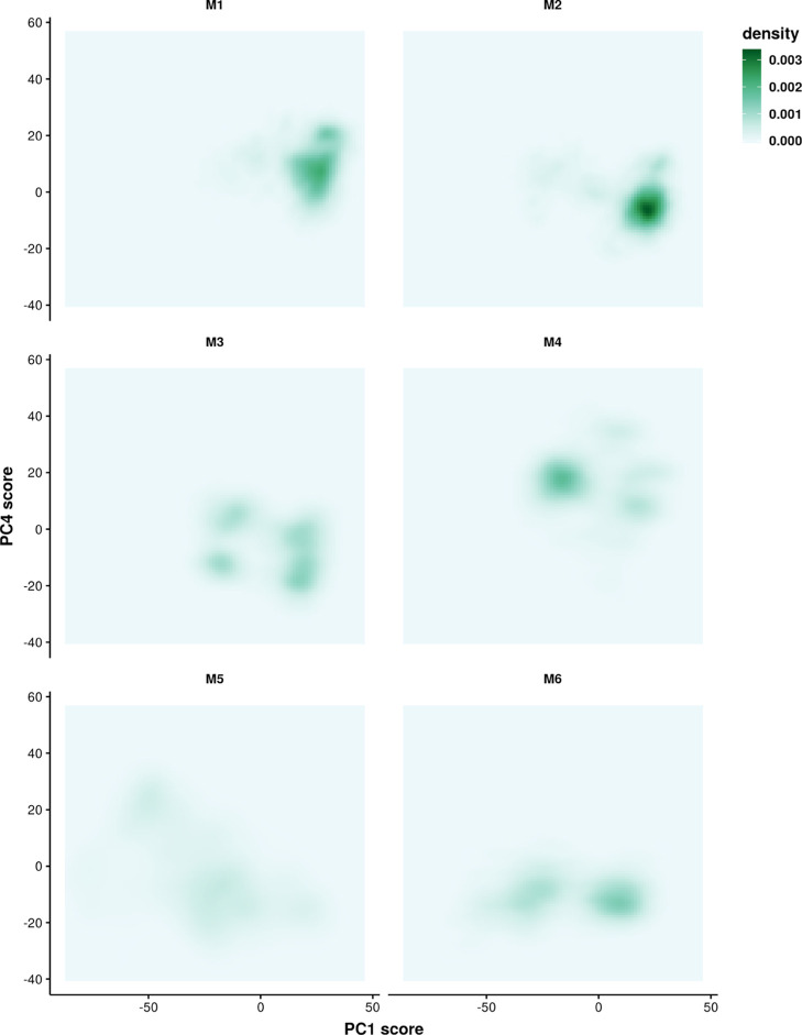
To investigate the effect of selecting a limited number of predicted models on characterizing the aptamer by MD simulations, the structures from six groups of simulations were projected onto the phase space, which was defined by PCs. Figure 4 shows the probability distribution of the PC1 score. The PC1 score shows bimodal distributions in each group. Although the distributions among the groups are not exactly the same, there is a large overlap region among different groups of simulations. If the most frequently sampled region from potential energy distributions in Figure 1 is the global minimum, the conformations sampled by various groups starting from different predicted models should show a large overlap in this analysis. For better visualization, the conformational space was projected on two PCs that can best separate the groups of simulations. As shown in Table S1, PC4 shows the highest purity and normalized mutual information (NMI) when grouping all the structures into six clusters by Ckmeans.1d described earlier. PC1 ranks second for purity and NMI. The values of purity and NMI can also reflect the overlap of selected PCs from different groups. Hence, the 2D space of PC1 and PC4 is expected to better visualize the different regions sampled by the six groups of simulations. The goal here is to show that multiple independent simulations can sample more broadly than can be achieved by investigating the exact sampling overlap from different groups and to provide insights into the part of the RNA molecule that contributes the most to the differences. The loadings of PC1 and PC4 is plotted in Figure S5, which further explains that PC1 can be used to identify the loop region in the aptamer, and PC4 identifies the stem region. In Figure 5, each group might sample multiple regions on the PC space, for example, the M3 and M5 groups. There is an overlap region sampled by different groups, such as the dominant region sampled by M2 that is also explored by M3 and M6. It is noticeable that the simulations in the M5 group sample most broadly on the 2D space of PC1 and PC4. Part of the region that this group has sampled does not appear in other groups, such as the region around (−50, 20). In summary, multiple groups of simulations improve the sampling by exploring the phase space more broadly.

Figure 4.

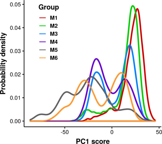
Probability distribution of PC1 score from different groups of simulations.

Figure 5.

Two-dimensional density of the structures sampled by each group projected on PC1 and PC4 space. Each group consists of 10 independent short simulations.

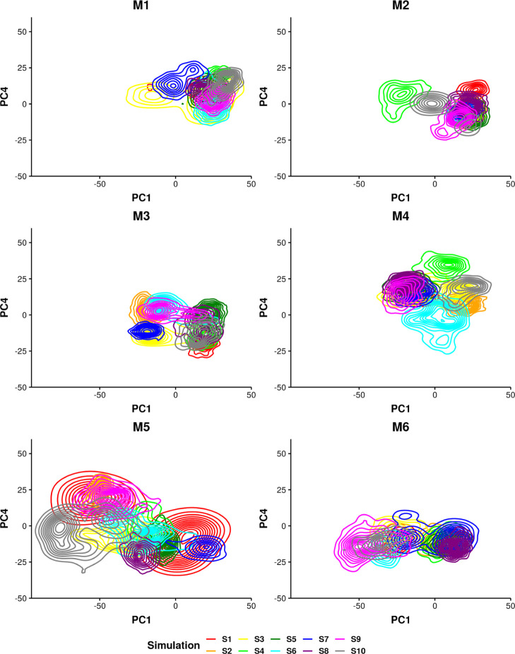
To further investigate whether the variations in sampling performance of different groups were due to statistical errors or different local energy landscapes of the various predicted models, the contours on the same phase space were plotted and colored differently for each simulation in Figure 6. This evaluation shows that independent simulations might visit different regions as well as overlap on the 2D space. For example, a part of the region sampled by S3 in the M1 group is also visited by other simulations in this group, while the region at PC1 less than 0 is only partially shared with S7. The M2 group shows similar sampling behavior including a popular region visited by most simulations except S4 and S10. While for other groups, multiple regions are visited by several simulations within the group, such as M3 and M6. Overall, group M5 sampled more broadly on the 2D PC space compared with other groups, for example the peaks at (−70, 0) contributed by S10 in the M5 group were not visited by other groups of simulations. It further explains that the region sampled by the M5 group appears lighter in the density plot (Figure 5). The M3, M5, and M6 groups explored a common region at PC4 less than 0, while this region was only visited by S6 in the M4 group. Regions not commonly visited by various groups tend to be from a few independent simulations within a group. The variations of sampling among the groups might have been the consequence of starting from different configurations from the structure prediction. Some simulations that sampled broadly in terms of potential energy in Figure S4 also appeared with multiple peaks in the 2D conformational space. For example, simulations S9 in the M2 group and S7 in the M6 group show two peaks on 2D PC projection. It indicates the aptamer goes through a conformational change in these simulations, which further results in crossing energy barriers. The contour plot confirms the variations between independent simulations from each group. It supports the necessity of performing multiple simulations from the same predicted structure as stated in the previous section. It further stresses the necessity to conduct multiple groups of simulations started from different configurations as different groups of simulations might sample different regions on the 2D PC space.

Figure 6.

Two-dimensional contour of structures sampled in each group projected on PC1 and PC4. The contour is colored by simulation.

To quantitatively examine the sampling from multiple groups, the recurrence rate was compared among the groups in Figure 7. The quantity % REC quantifies the percentage of the recurrence points in all points, and % DET measures the percentage of the diagonally adjacent recurrent points in all the recurrence points. The % REC varies among the groups of simulations (p-value = 0.03 < 0.05 from ANOVA), which results from the significant difference in the mean of groups M5 and M2 (p-value = 0.02 < 0.05 from Tukey’s honestly significant difference test). The % DET varies among the groups of simulations (p-value = 0.0014 < 0.05 from ANOVA) and group M5 exhibits a significantly different mean in comparison with other groups (p-value < 0.05 with groups M1, M2, M3, and M6 and p-value < 0.1 with group M4). The simulations starting in group M5 show larger % DET, which confirms the observation from Figure 3 that there are larger sequences of adjacent similar structures in individual simulations than between simulations. It also explains that the DL frequency in the M5 group shown in Figure 3 is contributed by most simulations in this group rather than by a few simulations. A possible reason for this finding is that some simulations in the M5 group underwent conformational transition, crossing the energy barrier(s) earlier than simulations in other groups and entering a local energy minimum, which resulted in diverse sampling in M5. Together, the information from Figures 5 and 6 shows that the M5 group sampled a broader region because of there being less overlap of independent simulations in this group. Over a limited timescale, the simulations in M5 are relatively more conserved. The results of group M5 indicate that the sampling might be related to the initial conditions of the simulations in this group. In summary, the projection on the 2D PC space and recurrence rate provides insight into the necessity to start multiple groups of simulations from different configurations, which refers to different predicted models in this study.

Figure 7.

Percent recurrence from the six groups of 10 independent short simulations. The left panel shows the overall percent recurrence and the right panel shows the percent diagonal recurrence.

To further investigate the dependence of sampling variation on the initial configurations among the groups, the largest Lyapunov exponent was calculated to study the dependence of a chaotic system on the initial conditions. In Figure 8, the largest Lyapunov exponent, calculated for each simulation by measuring the distance of the segment with its neighbor orbits evolving along the trajectory, was compared among different groups. The exponents measure the rate at which a system process creates or destroys information. The average largest Lyapunov exponents from each group were positive, which indicates that the simulations were chaotic in general. The largest Lyapunov exponents sampled from different groups are not from the populations with the same mean value (p-value = 0.0008 < 0.05 from ANOVA). It indicates the convergence of simulations depends on the initial conditions. Group M2 shows a significantly different mean value with groups M4, M5, and M6, which might have resulted from the simulations S3 and S7 having large values than any simulations in other groups. Some simulations in groups M5 and M6 show negative Lyapunov exponents, which indicates that the dynamics observed in these simulations are more converged than for other simulations. The reason for this might be because the regions on the energy landscapes sampled by the simulations of the M5 and M6 groups were basins with barriers difficult to overcome. The results here indicate that, for short simulations such as 100 ns simulations in this study, the convergence of simulations with the same length is different, which results from different relaxation times necessary for each simulation to reach equilibration. Hence, it is suggested to discard the pre-equilibration part of each trajectory for analysis.

Figure 8.

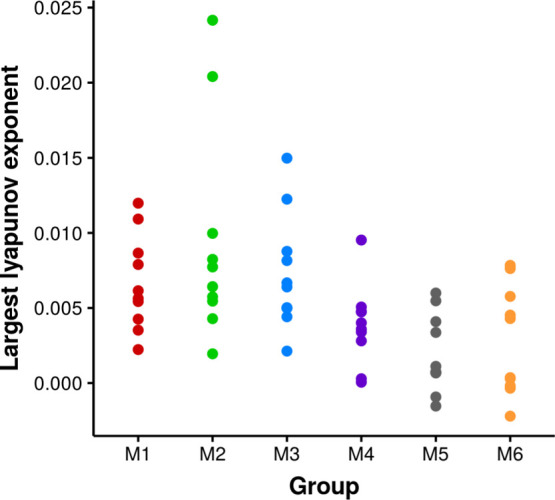
Chaotic behavior of the short simulations from the largest Lyapunov exponent colored by group.

Multiple Independent Simulations or a Single Long Simulation

In the previous section, results from multiple independent simulations from different groups reflect that this approach can obtain a more accurate average of a one-dimensional property of interest and capture fast transitions shown in the RP. To examine if multiple simulations can sample more broadly than a single long trajectory with equivalent length, the abovementioned analyses are repeated on a 1 μs trajectory.

The distribution of RNA potential energy from the 10 simulations is group M1 is compared with the long simulation started from the initial structure of M1 S1 in Figure 9. The long simulation enters a state that shows lower RNA potential energy. The results show that the aptamer structure in this specific simulation goes through large conformational transitions and reaches another equilibrium state, shown from the rmsd in Figure S6. One might argue that the 100 ns simulation does not reach the real equilibrium state because there is obvious conformational change from rmsd. To verify the long trajectory, a second 1 μs simulation was conducted by extending the simulation M2 S7. The rmsd of 100 ns M2 S7 simulation shows similar conformational change at the end of 100 ns trajectory (Figure S7). The RNA potential energy of M2 S7 from multiple short simulations and one long simulation also confirms the observation from M1 S1 simulations. In both cases, the long trajectory visits low RNA potential energy states that are not frequently sampled in the 10 independent short simulations.

Figure 9.

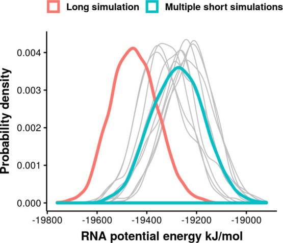
Comparison of RNA potential energy from 10 independent 100 ns simulations and 1 μs simulations. The distribution from each of the 10 simulations from group M1 is colored in gray. The distribution from all of these 10 simulations is plotted in red. The 1 μs long trajectory is started from the initial structure of M1 S1, colored in green.

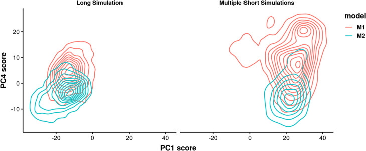
From here, it is necessary to know if the two 1 μs simulations converge to the same states. For structural visualization, the screenshots of the initial structures of these two simulations, average structures from 20 to 80 ns and average structures from 200 ns to 1 μs were compared in Figure 10. There is a large conformational change in the groove of both structures in the long 1 μs simulations, compared with the initial structures and states sampled in the first 100 ns. Comparing the two long trajectories, the flexible regions in this aptamer including the pentaloop and bulge exhibit different conformations, especially the bulge including bases C6 and A7. The base A7 is flipped out in M1 S1 while stacked in the bulge in M2 S7. To further investigate the sampling of the two long trajectories, the structures from two long simulations (taken every 200 ps) were aligned to the same structure as previous PCA analysis, and the coordinate data after superimposition were projected on the same eigenvectors previously obtained. The 2D PC projection in Figure 11 confirms that the long trajectories mainly sample different regions compared with multiple short simulations. It suggests that simulation timescale affects the dominant states captured by the trajectory. Conducting a single long simulation might be able to obtain an energetically favorable state. However, the structural fluctuations such as base flipping might require even much longer time to observe equilibrium. Hence, conducting multiple independent simulations is an efficient way to sample the diverse conformations that are expected in nucleic acid molecules that display dynamic changes in structure.

Figure 10.

Screenshots of structures from the M1 S1 simulation (pink) and M2 S7 simulation (green). The left panel shows initial structures. The middle panel shows the average structure from 20 to 80 ns as representative for 100 ns simulations. The right panel shows the average structures of the last 800 ns in 1 μs long trajectories.

Figure 11.

Comparison of the sampling from 10 independent short simulations and 1 long simulation on the 2D PC space. The left panel represents one long simulation extending M1 S1 (red) and M2 S7 (green) and the right panel represents 10 short simulations from group M1 (red) and M2 (green). A single long simulation might sample different regions with short simulations. Long simulations from different initial structures might also sample different regions and overlap regions.

It is noticeable that in Figure 11, group M1 and M2 show overlap regions on the 2D PC space both in 10 independent simulations and 1 long trajectory. It further stresses the necessity of conducting multiple simulations starting from different initial configurations that are as diverse as possible. It can be very computational expensive to conduct long trajectories from different initial configurations.

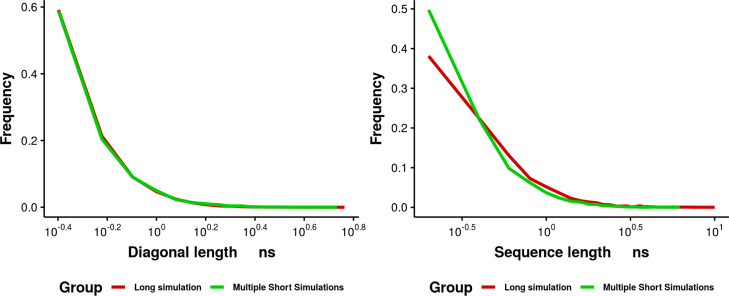
To further investigate whether the different sampling between multiple short simulations and one long simulation results from large conformational transitions that are missed by short simulations or a fast crossing of energy barriers, RQA was repeated for the long simulations to compare the sequential correlated structures in Figure 12. The 10 independent short simulations show consistent frequencies for DL. These short independent simulations also show a high fraction of single or short segments with sequential similar structures. However, the long trajectory shows a greater fraction of long sequential correlated structures. In summary, both multiple short simulations and a single long trajectory exhibit a long tail with consistent DL distribution. It indicates that short simulations are able to capture fast transitions. No obvious peak appears in the 1 μs trajectory that does not exist in the tail of 100 ns simulation distribution. It indicates the transition to the low RNA potential energy state observed in the long simulation results from relatively fast transitions that can be captured within 100 ns timescale. The greater fraction of long sequential similar structures in the 1 μs trajectory and greater SL that are not found in multiple short simulations indicate that in long simulation, the state with low RNA potential energy might be a stable state with deep basin.

Figure 12.

Frequency of DL (left) and SL (right) on the RP from multiple short simulations (green) and a single long simulation (red).

To investigate whether the structures sampled by the long 1 μs trajectory but not 100 ns simulations exist in other groups of simulations, all the structures are clustered via density-based clustering algorithm after dimension reduction via t-SNE. Compared with other clustering approaches, density-based cluster are capable of identifying metastable energy basins of arbitrary shape or size, not limited to Gaussian/hyperspheres.⁴⁸ The minimum number of points defined for DBSCAN clusters is 32, corresponding to 6.4 ns (as structures extracted every 200 ps from the simulations are used for analysis), which guarantees DL and SL reach stationary. The DBSCAN algorithm then identifies the number of clusters from the data adaptively.

The clustering results are reported in Figure 13, including 117 clusters in total. Most clusters (102 out of 117 clusters) are occupied by structures from one of the groups. The cells in the heatmap are colored by the fractions of the cluster members in each group. For the two long trajectories, no structures are grouped into the same cluster with 10 independent short simulations of M1 or M2, which indicates the equilibration part of the long simulations are sampling a different state with multiple short simulations.

Figure 13.

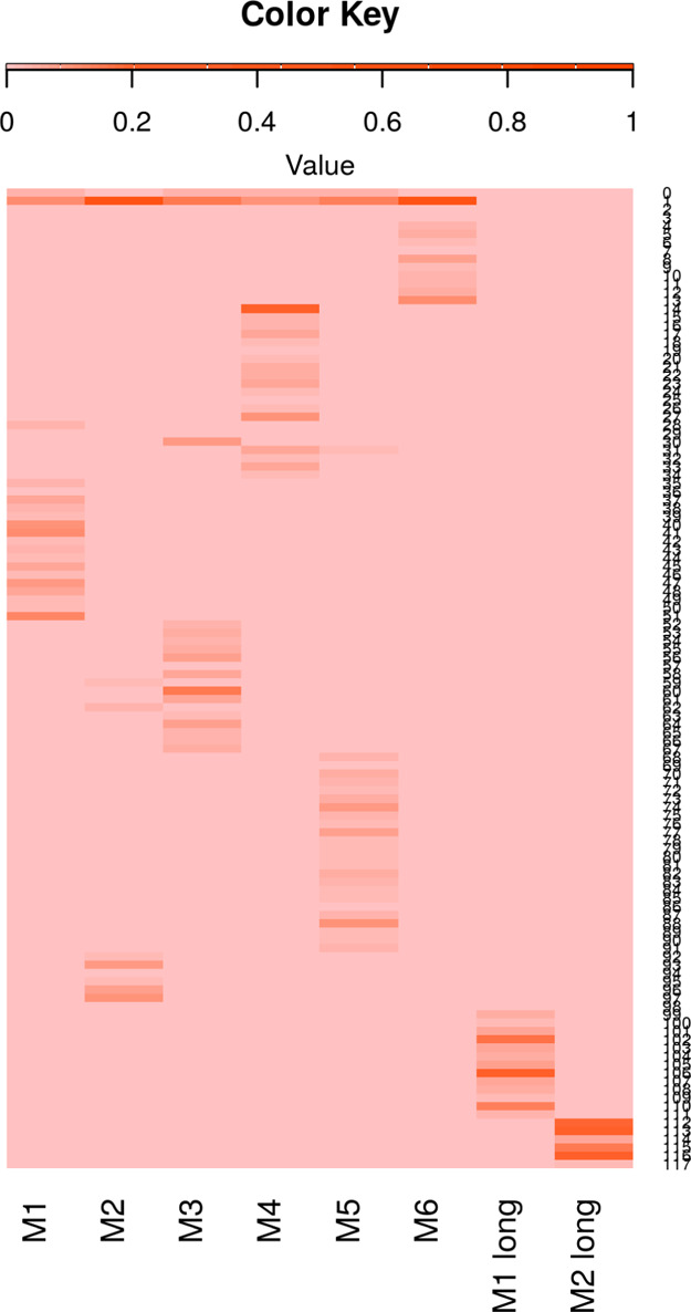
Density-based clustering on the MD simulations. The fraction of structures in the cluster in each group is colored from 0 in salmon and 1 in orange.

It is noticeable that there are no common structures from the two long simulations, except the structures determined as outliers. However, for the groups of 100 ns simulations, one large cluster include 63.2% of structures from group M2, 55.6% of structures from group M6, 15.5% of structures from group M3, 13.7% structures from groups M5, 12.0% of structures from group M1, and 10.5% structures from group M4. The results indicate that multiple short simulations are capable of sampling broadly, while the long trajectories are more likely to be trapped in a basin (Figure 13). Conducting long simulations needs extra caution and starting from different configurations can be of great importance.

Examining the Sampling Performance of all 60 Independent Simulations

The structures from the combination of all the 60 independent simulations were used to analyze the conformation of the aptamer. The root mean square fluctuations (RMSF) of the atoms in the aptamer were calculated to study the structure of the aptamer in this study in Figure 14. The RMSF from the pseudotrajectory concatenating all the 60 independent simulations is also compared with RMSF from each simulation in Figure 15. Examination of the RMSF shows high fluctuations with similar values in the bulge and pentaloop regions.

Figure 14.

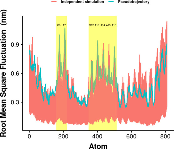
RMSF of the atoms in the aptamer. The residues C6 and A7 in the bulge and G12, A13, A14, A15, and A16 in the pentaloop are in the yellow shade. The green line represents the RMSF from the pseudotrajectory resulting from concatenating all the independent simulations. Red lines are from each of the 60 independent simulations.

Figure 15.

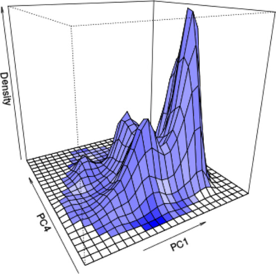
Density of structures from 60 MD simulations on PC1 and PC4 space, colored by the magnitude of potential energy with blue being high potential energy.

The conformations of aptamers strongly impact their functions. For further identification of the best aptamer conformations for binding the target molecule, molecular docking can be applied and a group of structures selected with the lowest binding free energy. By this means, structures favorable to target molecule binding can be identified.

The 2D density was constructed by interpolation on the PC1 and PC4 phase space in Figure 15. The potential energy value was used to color the landscape. This 2D landscape can identify less sampled regions, which might further inspire additional rounds of independent simulations to enhance sampling.

Conclusions

Multiple independent MD simulations were conducted using 3D RNA structure prediction for initial structures of an RNA aptamer to investigate the sampling performance.

We selected a feasible number of RNA 3D predicted models with diverse potential energy values. Multiple independent MD simulations were then carried out from each of these selected models. We found that with 10 independent simulations we were able to recover the RNA potential energy distribution with a low standard error. This result shows the promise of sampling compared with single simulations. We also demonstrated by RQA that 10 independent simulations could effectively sample the conformational transitions of the RNA aptamer.

We compared different groups of simulations starting from various predicted models. The conformational space projected on two selected PCs determined from PCA sampled by groups of simulations exhibited both overlap regions and distinct regions. These results satisfied the expectation of multiple independent simulations and further support the necessity to use various predicted structures when modeling an RNA aptamer with MD. The similarities and differences between simulations were further quantified by recurrence rate. Dependence on the initial conditions of the simulations was compared among the groups to develop an explanation for the differences in 2D conformational space. Combining all the simulations in this study, the conformations and dynamics of the aptamer were investigated. From the density on the 2D conformational space, the undersampled regions in the landscape were identified.

There are several avenues for further study. First, it would be helpful to know what the under-sampled region represents. The structures might be retrieved from PCA and tested for stability, which would provide insights as to whether the under-sampled region has a low probability of being visited in conformational space or if it is a consequence of bias in MD sampling. Second, it would be interesting to investigate the effect of initial structure selection on the overall sampling performance from multiple independent simulations for future simulation study design.

Methods

In this section, we describe how we simulated the RNA aptamer NEO2A using multiple independent MD simulations. We begin by presenting how we selected the initial structures for MD simulations from RNA 3D structure prediction. We then discuss our procedures to conduct multiple independent simulations of this aptamer. Finally, we describe the assessment of sampling performance qualitatively and quantitatively.

Structure Preparation

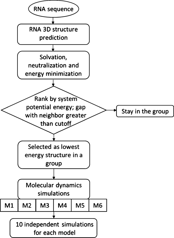
The MC-Fold|MC-Sym pipeline²⁵ was used to generate the NEO2A 3D structures from the sequence (CAC UGC AGU CCG AAA AGG GCC AGU G) and 137 models were obtained. Instead of selecting one structure with the lowest predicted energy, a feasible number of diverse structures were selected as the initial structures for multiple MD simulations in this study. The goal of using diverse initial structures is to enhance sampling via multiple independent simulations. The structures were solvated in water and neutralized by Na⁺ via GROMACS 5.0.5²⁶ using the Amber99sb²⁷ force field. After energy minimization, the potential energy of the system was recorded and used to rank the structures. To group the structures, a potential energy difference was calculated after ranking the structures from the lowest to the highest according to system potential energy. Structures with a potential energy difference greater than 10 kJ/mol were selected as the lowest energy structures in a new group. If a structure was found to be the only one in its grouping, it was counted as an outlier and excluded from the final selection of structures. The 137 structures were divided into six groupings, and the structures with lowest potential energy in each group were selected for MD simulations. The potential energy cutoff value at this step in the procedure could be adjusted depending on the desired group size and accuracy. The six models that were selected from the 137 predicted structures will be referred to as M1, M2, M3, M4, M5, and M6 in the order of the lowest to highest potential energy (Scheme 1).

Scheme 1. Workflow Used to Study the Conformation and Dynamics of RNA Aptamers from the Sequence.

The approach consists of three main steps, involving RNA 3D structure prediction from the sequence using MC-Fold|MC-Sym pipeline, model selection from the pool of predicted structures and multiple independent MD simulations using selected models as initial structures.

The NVT equilibration was carried out for energy-minimized models by velocity-rescale temperature coupling for 100 ps under 298 K with nucleic acid heavy atoms fixed. The NPT equilibrium was conducted with Parrinello-Rahman pressure coupling²⁸ and the same temperature coupling for 100 ps. To generate various initial structures that overcome local minima at a lower temperature more easily, the NPT equilibrium was conducted at 398 K for 100 ps. While at this high-energy state, 10 frames were selected at 10 ps increments to represent the structures at various positions on the free-energy landscape. Becausethese 10 frames were taken at an elevated temperature, the molecule could vary its state significantly enough to avoid being trapped in the same local minima. By this point, the 60 structures to be simulated and used for multiple independent simulations had been acquired.

Simulation Protocol

The 60 independent simulations were carried out with the following simulation protocol. The aptamer was centered in a cubic box of TIP3P water molecules.²⁹ The distance between the aptamer and the box was 20 Å. To neutralize the net charge of the aptamer, Na⁺ ions were randomly placed as counterions in the system. Particle mesh Ewald³⁰ was used for treating electrostatic interactions with a grid-spacing of 1.6 Å. The van der Waals interactions were treated with a short-range cutoff of 1.0 nm.

Energy minimization was conducted via the steepest descent method.³¹ The minimized structure was equilibrated with the NVT and NPT ensembles, respectively. The NVT thermal equilibration was carried out by velocity-rescaling temperature coupling for 100 ps at 298 K. The NPT equilibration was conducted with Parrinello-Rahman pressure coupling²⁸ and the same velocity-rescaling temperature coupling. During equilibration, position restraints were applied to nonhydrogen atoms of the aptamer. The LINCS algorithm³² was used to implement bond length constraints. The time step used was 2 fs, and periodic boundary conditions were applied to the system. Finally, an MD production simulation was carried out for 100 ns at constant temperature (298 K) and pressure (1.0 bar) with the aptamer, counterions and solvent molecules independently coupled to external heat baths with a relaxation time of 0.1 ps. System coordinates were saved from the trajectory at 2 ps intervals. Two 1 μs simulations were carried out by extending short simulations M1 S1 and M2 S7 to compare the sampling performance. All the 60 100 ns simulations were examined for equilibration by monitoring the moving average of RNA rmsd and radius of gyration. Simulations that explore new regions in conformational space during the 100 ns period observed from rmsd from initial structure were not included in the analysis. The pre-equilibration portion of the remaining simulations with unstable rmsd and radius of gyration was also discarded (details in Supporting Information).

Data Analysis

RMSF and the potential energy of only RNA aptamer were calculated with GROMACS.²⁶ A pseudotrajectory that combined 60 independent simulations with only RNA aptamer was constructed. Then, the structures were superimposed to a common structure (the first frame) by least square fitting to remove translation and rotation in GROMACS.²⁶

PCA was conducted on the x-, y-, and z-coordinates of 809 atoms in the aptamer saved every 200 ps from the pseudotrajectory. Coordinate data included 23,638 samples (structures extracted every 200 ps from each of the 60 simulations after discarding the pre-equilibration portion). All the structures were superimposed to one common structure, and all RNA atoms were included in the superimposition. All RNA atoms were included in the coordinate data for constructing covariance matrix in PCA. The coordinate data were first standardized (standardized data set with a mean of 0 and a standard deviation of 1). PCA were conducted via singular value decomposition (SVD) in an R package.³³ The equation for SVD of an m × n matrix X is the following

where U is an m × n matrix, S is an n × n diagonal matrix, and V^T is also an n × n matrix. When X is centered and the PCs are calculated from the covariance matrix, the eigenvalues are equivalent to s_k²/(n – 1).³⁴ The matrix V^T contains PCs and the matrix US is the score matrix. The loadings are given by columns of . The goal of PCA is to determine a low-dimensional set of coordinates onto which an informative projection can be made. The top 183 PCs explain 99% of the variation in the aptamer coordinates data. Hence, the top 183 PCs score data were used for further recurrence quantification.

To identify the PCs that can best separate structures from different groups of simulations, structures from all the simulations were clustered into six groups using PC score data via optimal one-dimensional clustering and compared with six groups of simulations via cluster evaluation. The clustering was carried out with an R package called Ckmeans.1d.dp³⁵ as a dynamic programming algorithm. The evaluation of clustering includes three external criteria of clustering quality. Purity is the fraction of the sum of the most frequent class from each cluster in the total number of samples

where Ω = {ω₁, ω₂, ..., ω_k} is the set of clusters, C = {c₁, c₂, ..., c_j} is the set of classes, and N is the total number of samples. In this study, the term “class” refers to the six groups of simulations. Purity varies between 0 for bad clustering and 1 for perfect clustering. However, high purity might result from a large number of clusters. NMI can overcome the misleading from the situation where each sample forms its own clusters

where I is the mutual information that measures the amount of information by which our knowledge about the classes increases when we are told what the clusters are. H is the entropy which fixes the problem because entropy tends to increase with the number of clusters. The value of NMI is between 0 and 1. The Rand index is defined as

A true positive (TP) means two similar samples (from the same class) are assigned to the same cluster, while a true negative (TN) means two dissimilar samples (from different classes) are assigned to different clusters. For a total number of N samples, RI looks into N(N – 1)/2 pairs of decisions. The PCs on which the projection of the aptamer coordinates achieving good clustering performance are selected for data visualization and potential energy landscape construction.

RQA^36,37 has been widely applied to dynamical system analysis in various scientific disciplines, for example behavioral and social sciences, medical science, and engineering.³⁸ MD simulations generate system observables at equidistant points in time, from which the characteristics about the underlying system dynamics can be extracted. The construction of RPs and RQA which extracts quantitative information from RPs is based on the idea of the phase space. This method allows us to extract information about system temporal correlations and chaotic behavior.³⁹ It was introduced to the analysis of MD simulations as an alternative analysis technique to obtain phase information about the energy landscape of simulated systems.^40,41 However, because of the high dimensionality of the biomolecular configuration space, it is necessary to apply multivariate recurrence-based methods to MD simulation data, which has the nature of multivariate time-series. More information on RQA can be found in tutorials.^42,43 Multidimensional RQA was conducted on the projection of coordinate data in each simulation on top 183 PCs to recover the nonlinear dynamics from PCA. By studying the recurrence–repetition of elements or patterns, the efficiency of sampling from multiple independent simulations can be measured. To recover higher-order dynamics, the method of time delayed embedding of the time series⁴⁴ was used. The embedding parameters include the embedding dimensions m, the delay d, the radius r, and the rescaling norm. The embedding dimension m is the integer global dimension that shows the necessary number of variables to unfold the dynamics from self-overlaps arising from projection. It was estimated with the method of false nearest neighbors. The time delay d was determined with average mutual information to create variables with lags. In this study, the delay d was calculated by average mutual information, and the embedding dimension m was estimated using false nearest neighbor.⁴⁵ For the PCs score data used in this study, after calculations on each PC score and further validation with multivariate data via the method from Wallot and Mønster,⁴⁶ we decided not to embed, hence, m = 1 and d = 1. The radius r is the threshold within which two samples are counted as being recurrent. The radius r in this study was set so that the resulting percent recurrence (% REC) of the coordinate data randomly sampled from pseudotrajectory was 5%. The goal here was to use data randomly sampled from the pseudotrajectory as a baseline to study the recurrence quantities in individual simulations and compare the sampling performance. These quantities included % REC, percent determinism (% DET), average size of shared patterns (average diagonal line), and average SL (ASL) of each data point.

To investigate the sensitivity of initial configurations, the chaotic properties of this aptamer system were identified by Lyapunov exponents. Lyapunov exponents are the average exponential rates of divergence or convergence of nearby orbits in phase space. The Lyapunov exponent is calculated with the approach developed by Wolf et al.⁴⁷ Each structure in the simulation is a d-dimensional vector, y(n) = [x₁, x₂, ..., x_d], n = 1, 2, ..., N. The nearest neighbor of y(n) can be found from the trajectory, denoted as y(n; 0). The nearest neighbor y(0; 0) of the initial structure y(0) was identified as the start of neighboring orbit by measuring the Euclidean distance L(t₀). The temporal separation between this nearest neighbor and the initial structure in the original trajectory was also monitored because a pair of points with a much smaller temporal separation is characterized by a zero Lyapunov exponent. After evolution time t₁, the initial length will have evolved to L′(t₁) [the distance between y(0; t₁) and y(t₁)]. The evolution time t₁ is supposed to be short enough so that only small-scale structures, such as aptamers, are likely to be examined. It is suggested to avoid too large evolution time because of possible L′ shrinkage, when the trajectories passing through a folding region. A new structure is then selected as y(t₁;0), which satisfies two criteria: its separation L(t₁) from y(t₁) is small, and the angular separation between y(t₁;0) and y(0; t₁) is small. If y(t₁;0) cannot be found, the points being used are retained. The procedure is repeated until the fiducial trajectory evolves to the end. The largest Lyapunov exponent is then calculated from

where M is the total number of replacement steps. When the nearest neighbor of the initial structure in the original trajectory was close to the end, the second nearest neighbor of the initial structure was selected for the calculation.

All the structures, including 60 independent short simulations and two long simulations, were clustered to study if the states visited by long simulations can be sampled by short simulations. The coordinate projection on the top 193 PCs from PCA that describes 99% of the variance were used in the analysis. Structures from two long trajectories were also projected onto the 193 PCs. The 193 PCs were processed for further dimension reduction via t-distributed stochastic neighbor embedding (t-SNE).⁴⁸ This approach optimizes the one-to-one mapping of high dimensional objects to a 2D space by reproducing joint Gaussian probabilities in high-dimensional space with a heavy-tail Student t-distributed 2D space.⁴⁹ In this step, only points that are extremely close in the high-dimensional conformation space lie in close proximity to each other in the 2D-reduced space. Density-based clustering was conducted on the 2D data from t-SNE using the DBSCAN algorithm. The minimum number of points, which is a required input for DBSCAN, was defined based on the frequency of the DL from the RP. The number of structures that correspond to 6.4 ns was defined as the minimum number of points required to form a cluster, which corresponds to DL reaching a relatively low frequency. The radius of the hypersphere defining the neighborhood in DBSCAN was obtained by computing the k-nearest neighbor distances. The analysis was conducted using R package Rtsne⁵⁰ and dbscan.⁵¹

Supporting Information Available

The Supporting Information is available free of charge at https://pubs.acs.org/doi/10.1021/acsomega.0c01867.

• Screenshot of 60 initial structures of MD simulations in this study; rmsd matrix of the initial structures of 60 independent MD simulations; RNA potential energy distribution from 10 independent simulations; probability distribution of RNA potential energy calculated from each independent simulation; top 5 PCs from 1D clustering assessment; loadings of PC1 (left) and PC4 (right), colored by different regions of the RNA aptamer; rmsd of 100 ns simulation M1 S1 (left) and 1 μs simulation extending M1 S1 (right); and rmsd of 100 ns simulation M2 S7 (left) and 1 μs simulation extending M2 S7 (right) (PDF)

The authors declare no competing financial interest.

References

- Klussmann S.The Aptamer Handbook: Functional Oligonucleotides and Their Applications; Wiley-VCH, 2006. [Google Scholar]
- Rhinehardt K. L.; Srinivas G.; Mohan R. V. Molecular Dynamics Simulation Analysis of Anti-MUC1 Aptamer and Mucin 1 Peptide Binding. J. Phys. Chem. B 2015, 119, 6571–6583. 10.1021/acs.jpcb.5b02483. [DOI] [PubMed] [Google Scholar]
- Cruz J. A.; Blanchet M.-F.; Boniecki M.; Bujnicki J. M.; Chen S.-J.; Cao S.; Das R.; Ding F.; Dokholyan N. V.; Flores S. C.; Huang L.; Lavender C. A.; Lisi V.; Major F.; Mikolajczak K.; Patel D. J.; Philips A.; Puton T.; Santalucia J.; Sijenyi F.; Hermann T.; Rother K.; Rother M.; Serganov A.; Skorupski M.; Soltysinski T.; Sripakdeevong P.; Tuszynska I.; Weeks K. M.; Waldsich C.; Wildauer M.; Leontis N. B.; Westhof E. RNA-Puzzles: A CASP-like Evaluation of RNA Three-Dimensional Structure Prediction. RNA 2012, 18, 610–625. 10.1261/rna.031054.111. [DOI] [PMC free article] [PubMed] [Google Scholar]
- Miao Z.; Adamiak R. W.; Antczak M.; Batey R. T.; Becka A. J.; Biesiada M.; Boniecki M. J.; Bujnicki J. M.; Chen S.-J.; Cheng C. Y.; Chou F.-C.; Ferré-D’Amaré A. R.; Das R.; Dawson W. K.; Ding F.; Dokholyan N. V.; Dunin-Horkawicz S.; Geniesse C.; Kappel K.; Kladwang W.; Krokhotin A.; Łach G. E.; Major F.; Mann T. H.; Magnus M.; Pachulska-Wieczorek K.; Patel D. J.; Piccirilli J. A.; Popenda M.; Purzycka K. J.; Ren A.; Rice G. M.; Santalucia J.; Sarzynska J.; Szachniuk M.; Tandon A.; Trausch J. J.; Tian S.; Wang J.; Weeks K. M.; Williams B.; Xiao Y.; Xu X.; Zhang D.; Zok T.; Westhof E. RNA-Puzzles Round III: 3D RNA Structure Prediction of Five Riboswitches and One Ribozyme. RNA 2017, 23, 655–672. 10.1261/rna.060368.116. [DOI] [PMC free article] [PubMed] [Google Scholar]
- Miao Z.; Adamiak R. W.; Blanchet M.-F.; Boniecki M.; Bujnicki J. M.; Chen S.-J.; Cheng C.; Chojnowski G.; Chou F.-C.; Cordero P.; Cruz J. A.; Ferré-D’Amaré A. R.; Das R.; Ding F.; Dokholyan N. V.; Dunin-Horkawicz S.; Kladwang W.; Krokhotin A.; Lach G.; Magnus M.; Major F.; Mann T. H.; Masquida B.; Matelska D.; Meyer M.; Peselis A.; Popenda M.; Purzycka K. J.; Serganov A.; Stasiewicz J.; Szachniuk M.; Tandon A.; Tian S.; Wang J.; Xiao Y.; Xu X.; Zhang J.; Zhao P.; Zok T.; Westhof E. RNA-Puzzles Round II: Assessment of RNA Structure Prediction Programs Applied to Three Large RNA Structures. RNA 2015, 21, 1066–1084. 10.1261/rna.049502.114. [DOI] [PMC free article] [PubMed] [Google Scholar]
- Ramachandran K. I.; Deepa G.; Namboori K.. Computational Chemistry and Molecular Modeling: Principles and Applications; Springer-Verlag: Berlin Heidelberg, 2008. [Google Scholar]
- Leach A. R.Molecular modelling: principles and applications. Prentice Hall: Harlow, England, 2001.
- Zuckerman D. M. Equilibrium Sampling in Biomolecular Simulations. Annu. Rev. Biophys. 2011, 40, 41–62. 10.1146/annurev-biophys-042910-155255. [DOI] [PMC free article] [PubMed] [Google Scholar]
- Lyman E.; Zuckerman D. M. On the Structural Convergence of Biomolecular Simulations by Determination of the Effective Sample Size. J. Phys. Chem. B 2007, 111, 12876–12882. 10.1021/jp073061t. [DOI] [PMC free article] [PubMed] [Google Scholar]
- Lyman E.; Zuckerman D. M. Ensemble-Based Convergence Analysis of Biomolecular Trajectories. Biophys. J. 2006, 91, 164–172. 10.1529/biophysj.106.082941. [DOI] [PMC free article] [PubMed] [Google Scholar]
- Grossfield A.; Patrone P. N.; Roe D. R.; Schultz A. J.; Siderius D.; Zuckerman D. M. Best Practices for Quantification of Uncertainty and Sampling Quality in Molecular Simulations [Article v1.0]. Living J. Comput. Mol. Sci. 2019, 1, 5067. 10.33011/livecoms.1.1.5067. [DOI] [PMC free article] [PubMed] [Google Scholar]
- Grossfield A.; Zuckerman D. M. Quantifying Uncertainty and Sampling Quality in Biomolecular Simulations. Annu. Rep. Comput. Chem. 2009, 5, 23–48. 10.1016/S1574-1400(09)00502-7. [DOI] [PMC free article] [PubMed] [Google Scholar]
- Perez J. J.; Tomas M. S.; Rubio-Martinez J. Assessment of the Sampling Performance of Multiple-Copy Dynamics versus a Unique Trajectory. J. Chem. Inf. Model. 2016, 56, 1950–1962. 10.1021/acs.jcim.6b00347. [DOI] [PubMed] [Google Scholar]
- Pranami G.; Lamm M. H. Estimating Error in Diffusion Coefficients Derived from Molecular Dynamics Simulations. J. Chem. Theory Comput. 2015, 11, 4586–4592. 10.1021/acs.jctc.5b00574. [DOI] [PubMed] [Google Scholar]
- Bowman G. R.; Ensign D. L.; Pande V. S. Enhanced Modeling via Network Theory: Adaptive Sampling of Markov State Models. J. Chem. Theory Comput. 2010, 6, 787–794. 10.1021/ct900620b. [DOI] [PMC free article] [PubMed] [Google Scholar]
- Zimmerman M. I.; Bowman G. R. FAST Conformational Searches by Balancing Exploration/Exploitation Trade-Offs. J. Chem. Theory Comput. 2015, 11, 5747–5757. 10.1021/acs.jctc.5b00737. [DOI] [PubMed] [Google Scholar]
- Zimmerman M. I.; Porter J. R.; Sun X.; Silva R. R.; Bowman G. R. Choice of Adaptive Sampling Strategy Impacts State Discovery, Transition Probabilities, and the Apparent Mechanism of Conformational Changes. J. Chem. Theory Comput. 2018, 14, 5459–5475. 10.1021/acs.jctc.8b00500. [DOI] [PMC free article] [PubMed] [Google Scholar]
- Aytenfisu A. H.; Liberman J. A.; Wedekind J. E.; Mathews D. H. Molecular Mechanism for PreQ1-II Riboswitch Function Revealed by Molecular Dynamics. RNA 2015, 21, 1898–1907. 10.1261/rna.051367.115. [DOI] [PMC free article] [PubMed] [Google Scholar]
- Gong Z.; Zhao Y.; Chen C.; Xiao Y. Role of Ligand Binding in Structural Organization of Add A-Riboswitch Aptamer: A Molecular Dynamics Simulation. J. Biomol. Struct. Dyn. 2011, 29, 403–416. 10.1080/07391102.2011.10507394. [DOI] [PubMed] [Google Scholar]
- Nguyen D. H.; Dieckmann T.; Colvin M. E.; Fink W. H. Dynamics Studies of a Malachite Green–RNA Complex Revealing the Origin of the Red-Shift and Energetic Contributions of Stacking Interactions. J. Phys. Chem. B 2004, 108, 1279–1286. 10.1021/jp037273b. [DOI] [Google Scholar]
- DePaul A. J.; Thompson E. J.; Patel S. S.; Haldeman K.; Sorin E. J. Equilibrium Conformational Dynamics in an RNA Tetraloop from Massively Parallel Molecular Dynamics. Nucleic Acids Res. 2010, 38, 4856–4867. 10.1093/nar/gkq134. [DOI] [PMC free article] [PubMed] [Google Scholar]
- Warfield B. M.; Anderson P. C. Molecular Simulations and Markov State Modeling Reveal the Structural Diversity and Dynamics of a Theophylline-Binding RNA Aptamer in Its Unbound State. PLoS One 2017, 12, e0176229 10.1371/journal.pone.0176229. [DOI] [PMC free article] [PubMed] [Google Scholar]
- Wiehe K.; Schmidler S. C.. Monitoring Convergence of Molecular Simulations in the Presence of Kinetic Trapping; Citeseer, 2011. [Google Scholar]
- Shahlaei M.; Mousavi A. A Conformational Analysis Study on the Melanocortin 4 Receptor Using Multiple Molecular Dynamics Simulations. Chem. Biol. Drug Des. 2015, 86, 309–321. 10.1111/cbdd.12495. [DOI] [PubMed] [Google Scholar]
- Parisien M.; Major F. The MC-Fold and MC-Sym Pipeline Infers RNA Structure from Sequence Data. Nature 2008, 452, 51–55. 10.1038/nature06684. [DOI] [PubMed] [Google Scholar]
- Abraham M. J.; Murtola T.; Schulz R.; Páll S.; Smith J. C.; Hess B.; Lindahl E. GROMACS: High Performance Molecular Simulations through Multi-Level Parallelism from Laptops to Supercomputers. SoftwareX 2015, 1–2, 19–25. 10.1016/j.softx.2015.06.001. [DOI] [Google Scholar]
- Lange O. F.; van der Spoel D.; de Groot B. L. Scrutinizing Molecular Mechanics Force Fields on the Submicrosecond Timescale with NMR Data. Biophys. J. 2010, 99, 647–655. 10.1016/j.bpj.2010.04.062. [DOI] [PMC free article] [PubMed] [Google Scholar]
- Nosé S.; Klein M. L. Constant Pressure Molecular Dynamics for Molecular Systems. Mol. Phys. 1983, 50, 1055–1076. 10.1080/00268978300102851. [DOI] [Google Scholar]
- Jorgensen W. L.; Chandrasekhar J.; Madura J. D.; Impey R. W.; Klein M. L. Comparison of Simple Potential Functions for Simulating Liquid Water. J. Chem. Phys. 1983, 79, 926–935. 10.1063/1.445869. [DOI] [Google Scholar]
- Essmann U.; Perera L.; Berkowitz M. L.; Darden T.; Lee H.; Pedersen L. G. A Smooth Particle Mesh Ewald Method. J. Chem. Phys. 1995, 103, 8577–8593. 10.1063/1.470117. [DOI] [Google Scholar]
- Leach A. R.5.4.1 The Steepest Descent Method. Molecular Modelling: Principles and Applications; Prentice Hall: Harlow, England; New York, 2001; p 262. [Google Scholar]
- Hess B.; Bekker H.; Berendsen H. J. C.; Fraaije J. G. E. M. LINCS: A Linear Constraint Solver for Molecular Simulations. J. Comput. Chem. 1997, 18, 1463.. [DOI] [Google Scholar]
- R: The R Project for Statistical Computing https://www.r-project.org/ (accessed Jul 7, 2018).
- Wall M. E.; Rechtsteiner A.; Rocha L. M.. Singular Value Decomposition and Principal Component Analysis, 2002. arXiv:physics/0208101. [Google Scholar]
- Wang H.; Song M. Ckmeans.1d.Dp: Optimal k-Means Clustering in One Dimension by Dynamic Programming. R J. 2011, 3, 29–33. 10.32614/rj-2011-015. [DOI] [PMC free article] [PubMed] [Google Scholar]
- Eckmann J.-P.; Kamphorst S. O.; Ruelle D. Recurrence Plots of Dynamical Systems. EPL 1987, 4, 973–977. 10.1209/0295-5075/4/9/004. [DOI] [Google Scholar]
- Zbilut J. P.; Webber C. L. Embeddings and Delays as Derived from Quantification of Recurrence Plots. Phys. Lett. A 1992, 171, 199–203. 10.1016/0375-9601(92)90426-M. [DOI] [Google Scholar]
- Marwan N.; Webber C. L.; Macau E. E. N.; Viana R. L. Introduction to Focus Issue: Recurrence Quantification Analysis for Understanding Complex Systems. Chaos 2018, 28, 085601. 10.1063/1.5050929. [DOI] [Google Scholar]
- Karakasidis T. E.; Fragkou A.; Liakopoulos A. System Dynamics Revealed by Recurrence Quantification Analysis: Application to Molecular Dynamics Simulations. Phys. Rev. E: Stat., Nonlinear, Soft Matter Phys. 2007, 76, 021120. 10.1103/PhysRevE.76.021120. [DOI] [PubMed] [Google Scholar]
- Giuliani A.; Manetti C. Hidden Peculiarities in the Potential Energy Time Series of a Tripeptide Highlighted by a Recurrence Plot Analysis: A Molecular Dynamics Simulation. Phys. Rev. E: Stat. Phys., Plasmas, Fluids, Relat. Interdiscip. Top. 1996, 53, 6336–6340. 10.1103/physreve.53.6336. [DOI] [PubMed] [Google Scholar]
- Manetti C.; Ceruso M.-A.; Giuliani A.; Webber C. L. Jr.; Zbilut J. P. Recurrence Quantification Analysis as a Tool for Characterization of Molecular Dynamics Simulations. Phys. Rev. E: Stat. Phys., Plasmas, Fluids, Relat. Interdiscip. Top. 1999, 59, 992–998. 10.1103/PhysRevE.59.992. [DOI] [Google Scholar]
- Wallot S. Recurrence Quantification Analysis of Processes and Products of Discourse: A Tutorial in R. Discourse Process 2017, 54, 382–405. 10.1080/0163853X.2017.1297921. [DOI] [Google Scholar]
- Wallot S.; Leonardi G. Analyzing Multivariate Dynamics Using Cross-Recurrence Quantification Analysis (CRQA), Diagonal-Cross-Recurrence Profiles (DCRP), and Multidimensional Recurrence Quantification Analysis (MdRQA) – A Tutorial in R. Front. Psychol. 2018, 9, 2232. 10.3389/fpsyg.2018.02232. [DOI] [PMC free article] [PubMed] [Google Scholar]
- Takens F.Detecting Strange Attractors in Turbulence. In Dynamical Systems and Turbulence, Warwick 1980; Rand D., Young L.-S., Eds.; Lecture Notes in Mathematics; Springer Berlin Heidelberg, 1981; pp 366–381. [Google Scholar]
- Abarbanel H.Analysis of Observed Chaotic Data; Springer Science & Business Media, 2012. [Google Scholar]
- Wallot S.; Mønster D. Calculation of Average Mutual Information (AMI) and False-Nearest Neighbors (FNN) for the Estimation of Embedding Parameters of Multidimensional Time Series in Matlab. Front. Psychol. 2018, 9, 1679. 10.3389/fpsyg.2018.01679. [DOI] [PMC free article] [PubMed] [Google Scholar]
- Wolf A.; Swift J. B.; Swinney H. L.; Vastano J. A. Determining Lyapunov Exponents from a Time Series. Phys. D 1985, 16, 285–317. 10.1016/0167-2789(85)90011-9. [DOI] [Google Scholar]
- Dethoff E. A.; Petzold K.; Chugh J.; Casiano-Negroni A.; Al-Hashimi H. M. Visualizing Transient Low-Populated Structures of RNA. Nature 2012, 491, 724–728. 10.1038/nature11498. [DOI] [PMC free article] [PubMed] [Google Scholar]
- Chattopadhyay A.; Zheng M.; Waller M. P.; Priyakumar U. D. A Probabilistic Framework for Constructing Temporal Relations in Replica Exchange Molecular Trajectories. J. Chem. Theory Comput. 2018, 14, 3365–3380. 10.1021/acs.jctc.7b01245. [DOI] [PubMed] [Google Scholar]
- Rtsne: T-Distributed Stochastic Neighbor Embedding using a Barnes-Hut Implementation version 0.15 from CRAN https://rdrr.io/cran/Rtsne/ (accessed Feb 19, 2020).
- Hahsler M.; Piekenbrock M.; Doran D. Dbscan: Fast Density-Based Clustering with R. J. Stat. Software 2019, 91, 1–30. 10.18637/jss.v091.i01. [DOI] [Google Scholar]
Associated Data
This section collects any data citations, data availability statements, or supplementary materials included in this article.