Ocean currents promote rare species diversity in protists

Transport by ocean currents contributes to the diversity of planktonic species observed in metagenomic studies.

Abstract

Oceans host communities of plankton composed of relatively few abundant species and many rare species. The number of rare protist species in these communities, as estimated in metagenomic studies, decays as a steep power law of their abundance. The ecological factors at the origin of this pattern remain elusive. We propose that chaotic advection by oceanic currents affects biodiversity patterns of rare species. To test this hypothesis, we introduce a spatially explicit coalescence model that reconstructs the species diversity of a sample of water. Our model predicts, in the presence of chaotic advection, a steeper power law decay of the species abundance distribution and a steeper increase of the number of observed species with sample size. A comparison of metagenomic studies of planktonic protist communities in oceans and in lakes quantitatively confirms our prediction. Our results support that oceanic currents positively affect the diversity of rare aquatic microbes.

INTRODUCTION

Oceanic plankton can be transported across very large distances by currents. Many planktonic species are cosmopolitan, i.e., they are found virtually everywhere across the global ocean (1). These observations suggest that, at first sight, the distribution of planktonic species is not limited by dispersal and, therefore, that niche preference is the predominant factor determining species abundance (2). However, in the presence of a limited set of resources, niche theory predicts species-poor communities. In contrast, planktonic communities in the oceans are very diverse (3–6). This contradiction of the basic principles of niche theory (7) has puzzled ecologists for decades (8) and has fostered numerous attempts to explain the diversity of plankton (9). One proposal is that variable environments offer more possibilities for specialization of ecological traits (4, 10–14). Another proposal is that chaotic advection by oceanic currents creates barriers reducing competition among species, therefore promoting species coexistence (15, 16). Quantitative analyses also suggest that oceanic currents play an important role in organizing large-scale diversity patterns (17, 18) and that dispersal limitation contributes, alongside with niche specialization, to the microbial biodiversity of oceans (19–23). The influence of oceanic currents on biodiversity patterns of planktonic communities can be tested by a comparison of oceans and lakes, in which currents are reduced.

DNA metabarcoding has allowed rapid and extensive measurements of the diversity of aquatic microbial communities, providing new means to study the ecological forces shaping planktonic communities. Metabarcoding studies have revealed that, besides commonly observed species, planktonic communities are characterized by a vast range of rare species. This so-called rare biosphere (24, 25) makes up the majority of planktonic species (21, 26) and is the subject of our study. The diversity of planktonic species can be quantified by the species abundance distribution (SAD), defined as the frequency P(n) of species with abundance n in a sample. SADs of rare marine protists are qualitatively different from those of abundant species (27, 28) and appear to follow a power law distribution

$$P(n)\propto 1/n^{\mathrm{\alpha }}$$ (1)

The exponent α varies significantly among samples, is weakly correlated with environmental factors, and is significantly larger than 1 on average (29). Diversity patterns in other microbial communities, such as that of the human gut (30), are well described by a form of SAD following the Fisher log series, P(n) ∝ e^{−c n}/n (31), as predicted by Hubbell’s neutral model (31). For large communities, the parameter c is very small, so that the distribution is close to a power law with α = 1. Hubbell’s neutral model is therefore unable to explain the steep decay of SADs in the rare oceanic biosphere. This steep decay can be obtained with a modified neutral model that takes into account density dependence of growth and death rates (29, 32–34). However, the ecological forces determining this density dependence in the oceans are unknown.

Here, we propose that the steep decay of SADs observed in the oceans is caused by the particular way chaotic advection by oceanic currents limits dispersal. Oceanic currents affect distributions of planktonic populations by stirring and mixing. At the submesoscale, oceanic currents also affect ecological interactions, light exposure, and nutrient upwelling (35). Previous theoretical studies have shown that currents can affect effective population size (36) and provoke counterintuitive effects on fixation times (37), particularly in the presence of divergent flows (38, 39). However, these studies did not scrutinize the effects of advection on multispecies communities. To test our hypothesis, we introduce a model that takes into account the role of transport by oceanic currents in determining the genealogy of microbes in a sample. Our model predicts that, in the presence of chaotic advection, SADs are characterized by larger values of the exponent α. It also predicts that chaotic advection causes a sharper increase of species diversity as a function of sample size. To validate these results, we analyze 18S ribosomal RNA (rRNA) sequencing data generated from oceanic water samples (29). We compare these results with sequencing data from lake protist communities (40). The observations quantitatively match our predictions, supporting the idea that chaotic advection by oceanic currents is responsible for the differences in biodiversity patterns between oceans and lakes.

RESULTS

Coalescence model predicts the effect of chaotic advection by oceanic currents on SADs

We introduce a computational model to assess the effect of chaotic advection on the protist species distribution of a water sample. In this model, we assign a Lagrangian tracer (hereafter “tracer”) to each individual in the sample (see Fig. 1). Tracers are initially placed in a local area, representing the portion of water where the sample was collected. The spatial coordinates x and y of each tracer move backward in time, following the spatial trajectory of the ancestors of each individual (see Fig. 1). If two tracers are at a sufficiently close distance, then they coalesce into a single tracer with a given probability. This new tracer represents the common ancestor of the two individuals. Last, tracers are assigned at a fixed rate μ to one species. These events represent immigration due to other causes than ocean currents. Assigned tracers are eliminated from the system. At the end of a run, individuals in the original sample are considered conspecific if their corresponding tracers have coalesced to a common ancestor before being eliminated (see Materials and Methods, Fig. 1, and movie S1). This coalescence model can be interpreted as the backward version of an individual-based community model, which includes advection by currents (see fig. S1) (38, 41). The coalescent formulation has the advantage of describing the dynamics of one sample embedded in a larger ecosystem (42, 43).

Fig. 1. Genealogy in oceanic currents.

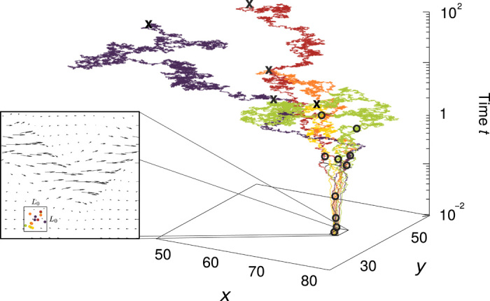
(Left) The coalescence model predicts the protist species composition in a sample of oceanic water taken from an area of size L₀ × L₀. Different colors represent different species. Arrows represent the velocity field induced by ocean currents. (Right) Trajectories of the coalescence model with ocean currents. Individuals are represented by tracers that are transported backward in time and can coalesce with other tracers if they reach a close distance. Coalescence events are marked by open circles; trajectories of individuals that have coalesced are shown in the same color. Tracers are removed from the population at an immigration rate μ (marked by crosses). See also movie S1.

We simulate the coalescence model with and without oceanic currents. In the latter case, movements of tracers are modeled as a simple diffusion process, taking into account individual movements and small-scale turbulence. In the former case, we superimpose to this diffusion process the effect of large-scale oceanic currents. We model transport by these currents with a kinematic model of a meandering jet, which is a common large-scale structure characterizing oceanic flows (44, 45). Population sizes and parameters characterizing the flow are sampled in a physically realistic range (see Materials and Methods) (45). All other parameters characterizing population dynamics are chosen identically in the two cases (see Materials and Methods).

SADs predicted by the model present a considerable variability depending on parameters and demographic stochasticity, both in the presence and absence of currents (see Fig. 2, A and B). To characterize individual SAD curves, we fit them with a power law function P(n) ∝ 1/n^α using maximum likelihood in an optimal range of abundances (see Materials and Methods). For comparison, we also fit an exponential distribution P(n) ∝ e^{−c n} and a Fisher log series P(n) ∝ e^{−c n}/n in the same range. In most cases, the power law provides a better fit than the exponential distribution (74 and 77% of samples with and without currents, respectively) and than the Fisher log series (75 and 62% of samples with and without currents, respectively).

Fig. 2. Coalescence model predicts effect of chaotic advection by oceanic currents on SAD.

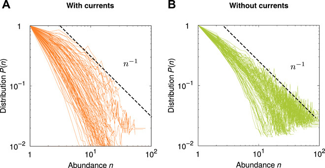
The two panels show SADs (A) in the presence (orange lines) and (B) absence (green lines) of oceanic currents for the coalescence model. Here and below, SAD curves are rescaled so that P(1) = 1 to ease visualization. Model details and parameters are presented in Materials and Methods. Dashed lines are power laws to guide the eye (see also Fig. 3).

Introducing oceanic currents in the model increases, on average, the steepness of SADs (see Fig. 2, A and B). We investigate the physical mechanisms causing this effect. One property of transport by currents is to enhance the effective diffusivity (46). We test whether effective diffusivity is responsible for the steepening of SADs by running our model with the effective diffusivity of the kinematic model but without currents. In this case, we find that the distribution of SAD exponent has lower average than in the case with smaller diffusion constant (see fig. S2). This implies that the increase of SAD exponents caused by currents is due to structures created by the flow that cannot be simplified into a diffusion process. We further run our model with a parameter choice yielding currents constant in time (see fig. S3). Neither in this case do we observe the steep SADs as that found in the presence of time-dependent currents.

These results suggest that the time-varying, chaotic nature of oceanic transport is responsible for the steepening of SAD curves. In particular, chaotic transport is often characterized by the presence of barriers limiting diffusion among certain regions of the flow. The presence of these barriers can be detected by finite-size Lyapunov exponents (FSLEs) (47). FSLEs quantify the growth rate of a finite separation among two particles advected by a flow. We measure local FLSEs for our model and find that they are significantly correlated with the spatial dependence of the exponent α (see fig. S4). This result supports the view that the long-lived barriers characterizing fluid flows prevent formation of large operational taxonomic units (OTUs) in the model and are thus responsible for the steepening of SAD curves.

Protist SADs are steeper in oceans than in freshwater

To test our predictions, we analyze DNA metabarcoding datasets from two studies of aquatic protists. The first dataset includes oceanic protist DNA sequences of 157 water samples from the TARA ocean expedition (29). The second dataset includes protist DNA sequences of 206 freshwater samples taken from lakes (40). We calculate SAD for each sample of both datasets using OTUs as proxies for species (see Materials and Methods). Here and in the following, if not stated otherwise, OTUs are built by clustering protist sequences at 97% sequence identity threshold. From now on, we discard “abundant species,” defined as those in abundance classes P(n) including less than four species. The remaining “rare species” are the subject of our study. They constitute 93% of all species in ocean samples and 78% of all species in lake samples.

As for the model, empirical SAD curves display considerable sample-to-sample variability, both in ocean and in freshwater samples (see Fig. 3). This variability is possibly caused by differences in ecological conditions among sampling sites. Empirical SAD curves are better fitted by a power law than by exponential or Fisher log series in most cases. The exponential distribution provides a better fit than the power law in 13% of lake samples and 13% of oceanic samples, whereas the Fisher log series provides better fits than the power law in 39% of lake samples and 18% of oceanic samples. We obtain similar results with different OTU definitions (95 and 99% instead of 97% similarity) and different thresholds separating abundant from rare species (see fig. S5). Notably, the power law decay of SADs is, on average, steeper in oceans than in lakes (see Fig. 3), as predicted by our coalescence model.

Fig. 3. Rare SADs present a steeper decay with abundance in oceans than in lakes.

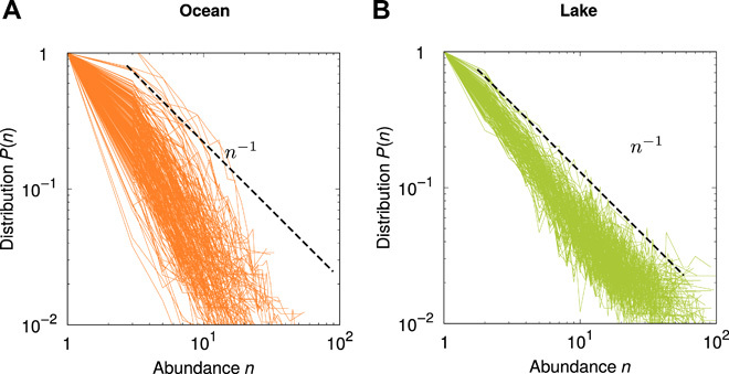
Continuous lines represent SADs of protist communities from (A) 157 oceanic samples (29) and (B) 206 freshwater samples (40). Total numbers of individuals in each sample are in the ranges of (A) (10³, 10⁵) and (B) (10⁴, 10⁶). In both panels, power laws (dashed lines) are shown to guide the eye.

Distribution of the SAD exponent is quantitatively predicted by the coalescence model.

We quantify the agreement between our model and the data by analyzing the distribution of the power law exponent α in Eq. 1. In the presence of currents, the model predicts a value of the exponent significantly larger than one (average α = 1.70, SD σ = 0.68). In the absence of oceanic currents, the model predicts an average α = 1.26, (σ = 0.46), a value compatible with the neutral prediction α = 1 in well-mixed systems (31) and spatially explicit neutral models (43). To verify whether the results are robust to oceanic current models, we also implement a kinematic model of the Adriatic sea and a chaotic Taylor-Green vortex (see fig. S6). In both cases, we obtain qualitatively similar results to that obtained for the meandering jet (see fig. S6), supporting that the observed mechanism is general.

Observations in both oceans and lakes are in excellent agreement with the distributions of exponents predicted by our model (see Fig. 4A). Our analysis confirms that the average exponent α is significantly larger than 1 in the oceans [average α = 1.79, σ = 0.52; see Fig. 4A and (29)]. In the lakes, the average exponent is α = 1.37 (σ = 0.44; see Fig. 4A). Adopting a different definition of OTUs (95 and 99% instead of 97%), different thresholds separating abundant from rare species and rarefying oceanic and lake data to the same sample size lead to qualitatively similar results (see fig. S5). In particular, the average exponent α in the oceans is between 4 and 23% larger than that in the lakes, depending on the threshold and the definition of OTUs (P values of Games-Howell test <0.002 in all cases).

Fig. 4. Power law exponents of SADs.

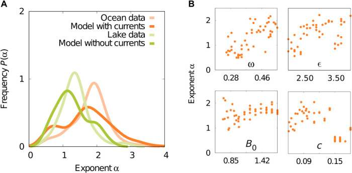
We run our models for different population sizes and different values of flux parameters for ocean samples (see Materials and Methods). We select 157 oceanic samples and 206 freshwater samples as in Fig. 3. We fit the power law exponent α of the SADs to the model and to the data using maximum likelihood. (A) Continuous distributions of the exponent obtained by kernel density estimation. (B) Dependence of the exponent on four main parameters of the oceanic flow: forcing frequency ω, wave perturbation amplitude ϵ, mean wave amplitude B₀, and phase speed c. In each subpanel, other parameters are kept constant (see Materials and Methods). Correlation tests of ω, ϵ, B₀, and c with the exponent α yield Pearson coefficients r_P = 0.72, 0.48, −0.04, and −0.58 and P values P = 3 × 10⁻⁹, 6 × 10⁻⁴, 0.77, 10⁻⁵, respectively.

The ocean (29) and lake (40) datasets we analyzed used different polymerase chain reaction (PCR) primers. To verify that this difference does not affect our results, we analyze two further metagenomic datasets, one from oceans (48) and one from lakes (49), that used the same primer. Also in this case, we find higher average exponent α in the oceans, confirming the robustness of our results (see fig. S7).

In the case of the meandering jet, we find that four parameters characterizing the shape and the mixing level of the jet mostly affect α. The value of the exponent is significantly correlated with the parameters ω, ϵ, and c (see Fig. 4B and fig. S8). In particular, the strong correlation with the forcing frequency ω driving the chaotic motion is a further evidence that the steepening of SAD exponents is caused by chaotic advection.

Chaotic advection by oceanic currents leads to a steeper increase in number of species as a function of sample size

By simulating our model at varying sample size N with and without currents, we predict that currents should significantly increase the number of expected species in each sample (see Fig. 5A). This effect is consistent with the increase of α in the presence of currents: Increasing α suppresses very abundant species and therefore increases the species diversity of the samples. This effect becomes more and more pronounced as N is increased. In the data, we find that samples from oceans contain more species than samples from lakes at similar sample size, which is consistent with our predictions (see Fig. 5A). The observed enrichment is even stronger than predicted by our model.

Fig. 5. Chaotic advection by oceanic currents increases species number S in a water sample.

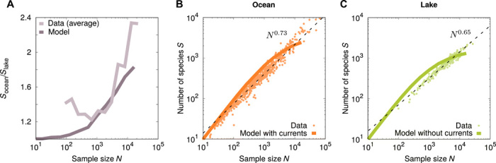
(A) Ratio S_ocean/S_lake as a function of the sample size N for the model and the data. We simulate the model at increasing sample sizes N in powers of 2 and obtain continuous curves by interpolation. Other parameters are presented in Materials and Methods. Averaged data are obtained by binning for both oceans and lakes. (B and C) Number of species S in samples of N individuals in (B) oceans and (C) lakes. A power law (Eq. 3) fits the data better than the Ewens sampling formula (Eq. 2) for both (B) oceanic (normalized log-likelihood −19.39 versus −449.52) and (C) lake samples (normalized log-likelihood −6.64 versus −117.21). Fitted exponents are z = 0.73 and z = 0.65 for oceans and lakes, respectively. The results of the coalescence model are shown with and without oceanic currents (orange and green lines, respectively). The Ewens sampling formula provides a better fit than the power law in both cases [normalized log-likelihood −420.95 versus −2131.43 in (B) and −434.66 versus −1902.62 in (C)].

We now study the increase of number of species with sample size in oceanic and lake water samples individually. In the case of well-mixed populations, the species composition of a given sample is described by the Ewens sampling formula (50), which predicts that the expected number of species in the sample is

$$S={\displaystyle \sum _{j=0}^N}\frac{\mathrm{\theta }}{\mathrm{\theta }+j-1}$$ (2)

where θ = 2N_effμ is the fundamental biodiversity number (31) and N_eff is the effective population size. Alternatively, sample species composition can be empirically described using a power law (51).

$$S\propto N^z$$ (3)

Our model predicts an increase in number of species with sample size, as predicted by the Ewens sampling formula (see Fig. 5, A and B). Both for ocean and freshwater samples, the power law model provides a better fit (see Fig. 5, A and B) with a higher exponent for oceanic samples (z = 0.73) compared to lake samples (z = 0.65). This result is qualitatively robust with respect to changing the OTU similarity threshold (see fig. 5C). Understanding why the observed number of species seems to depend on the sample size as a power law is an interesting question for future studies.

DISCUSSION

Oceanic currents are known to largely affect plankton distribution at large scale (15–17). Here, we show that chaotic advection by oceanic currents profoundly affects diversity of rare protist species even at the level of single metagenomic samples. Our coalescence model bridges the gap between large-scale oceanic dynamics and ecological dynamics at the individual level and provides a versatile and powerful tool to validate individual-based ecological models using DNA metabarcoding data. Although we focus on neutral dynamics of rare protists, our approach can be extended to more general ecological settings and to other plankton communities, including animals and prokaryotes. These generalizations, combined with high-throughput sequencing data, will permit to test whether the mechanism described here affects other kingdoms characterized by different population sizes, dispersal, and spatial turnover rates (52). These tests can shed light on the main ecological forces determining plankton dynamics and help understanding the difference in empirically observed patterns between abundant and rare species (24, 25).

The coalescence model predicts that the chaotic advection is responsible for steeper decay of SAD curves and steeper increase in the number of observed rare species with sample size. Both these predictions are in quantitative agreement with observations, although the exponent of the ocean and lake SADs largely overlap, suggesting that the trend is true globally but not necessarily so locally. The steep decay of SAD distributions in the oceans has been previously explained in terms of density-dependent effects (29). Although our study does not preclude this possibility, the comparison with freshwater ecosystems strongly suggests that chaotic advection effectively determines this density dependence. The steeper decay of SAD curves predicted by the coalescence model depends on geophysical parameters characterizing mixing. The irregular behavior of the SAD exponent as a function of these parameters (see Fig. 4B) potentially explains the fact that observed values of α appear weakly correlated with other physicochemical measurements at the sampling sites (29).

Chaotic flows, such as those considered here, are characterized by areas of strong mixing separated by barriers limiting transport. In our coalescence picture, these barriers reduce the pace of individual coalescence into species and therefore limit the formation of abundant species. Ecologically, this means that competition among individuals at opposite side of a barrier is reduced. This effective isolation prevents formation of very abundant species and therefore of SAD distributions with broader tails. A detailed physical theory of this phenomenon, building on recent advances on describing spatial neutral models (53, 43), remains a challenge for future studies.

In summary, our study provides a mechanistic theoretical framework to analyze diversity of rare microbial species in aquatic environments at the individual level. This paves the way to quantitatively understand how the chaotic advection by oceanic currents shapes the diversity of planktonic communities.

MATERIALS AND METHODS

Coalescence model

We consider N microbial individuals in an aquatic environment and seek to reconstruct their species identity. Each individual is associated with a Lagrangian tracer with two-dimensional spatial coordinates x and y. Initially, tracers are homogeneously distributed in a sample area $L_0\times L_0$, representing the place where the sample was collected. The tracers move in space according to the stochastic differential equations

$$\begin{array}{c}\frac{\mathrm{d}}{\mathrm{d}t}x=-u(x,y,t)+\sqrt{2D}{\mathrm{\xi }}_x(t)\\ \frac{\mathrm{d}}{\mathrm{d}t}y=-v(x,y,t)+\sqrt{2D}{\mathrm{\xi }}_y(t)\end{array}$$ (4)

where u and v are the components of an advecting velocity field representing the effect of oceanic currents. The velocity field has a minus sign since time runs backward: t = 0 is the time at which the sample was collected, and positive times correspond to the past history of the tracer. The terms proportional to $\sqrt{2D}$ are diffusion terms modeling individual movement and small-scale turbulence. The quantities ξ_x(t), ξ_y(t) are independent white noise sources satisfying 〈ξ_i(t)〉 = 0, 〈ξ_i(t)ξ_j(t^′)〉 = δ_ijδ(t − t^′) where 〈…〉 denotes an average and i, j ∈ (x, y). The advecting field u, v is specified in the next subsection.

To reconstruct the species identity of the tracers, we track their positions backward in time. Tracers at a short distance δ from each other at time t ≥ 0 can coalesce at a rate r. If this event occurs, then individuals in the sample represented by the two tracers descend from a common ancestor at time t in the past and therefore belong to the same species. We implement immigration events by assigning species at a rate μ. At each time step dt:

• 1)Each tracer moves from its position (x, y) to (x + Δx, y + Δy). The increments Δx, Δy are obtained by numerically integrating Eq. 4.
• 2)Tracers are selected one by one and are removed with probability μ dt (immigration event). Further, each tracer i can coalesce with probability r dt with any other tracer j present in an area of size δ × δ centered at the coordinates of tracer i.

We set r = 1, μ = 10⁻⁴, and the diffusion constant to D = 3 × 10⁻⁹, as further discussed below. The interaction distance δ is chosen to satisfy D = rδ², see (41). We take the linear size of the sample area on the order of the mean distance traveled by an individual in one generation, L₀ = 5 km, estimating a protist lifetime of about 1 day (54) and protist movements of about 20 km² day⁻¹ (55). Population size is randomly selected for each run in the range N ∈ (10³,10⁵) unless otherwise indicated. For Fig. 4B and movie S1, we set N = 8192.

Each simulation is run until all individuals have been assigned to OTUs by coalescence or immigration events. In the range of parameters we explored, the duration of a run is on the order of 100 years. However, most coalescence events occur on a much faster time scale (median of the coalescence times t ≈ 82 days for the ocean case and t ≈ 67 days for the freshwater case).

Kinematic model of the oceans

We model large-scale oceanic currents by means of a kinematic model of a meandering jet (44, 45). The velocity field u, v is defined in terms of a stream function. In a fixed reference frame, the stream function reads

$$\mathrm{\psi }(x\text{'},y\text{'},t\text{'})={\mathrm{\psi }}_0\{1-\text{tanh}(\frac{y\text{'}-A(t\text{'})\text{cos}[\mathrm{\kappa }(x\text{'}-c_{x}t\text{'})]}{\mathrm{\lambda }\sqrt{1+{\mathrm{\kappa }}^2{A}^2(t\text{'}){\text{sin}}^2[\mathrm{\kappa }(x\text{'}-c_{x}t\text{'})]}}\left)\right\}$$ (5)

The stream function is more conveniently written in a dimensionless form

$$\mathrm{\varphi }(x,y,t)=-\text{tanh}\left(\frac{y-B(t)\text{cos}(\mathit{kx})}{\sqrt{1+k^2{B}^2(t){\text{sin}}^2(\mathit{kx})}}\right)+\mathit{cy}$$ (6)

being B(t) = A(t′)/λ = B₀ + ϵcos (ωt + Φ), c = c_xL/ψ₀, and k = 2π/L, with L the meander wavelength. The transformation between dimensional and dimensionless units is x = (x^′ − c_xt)/λ, y = y^′/λ, and t = t^′ψ₀/λ² (44). The frame of reference of the dimensionless coordinates moves with the speed c_x of the jet. Given the stream function, the components of the velocity field in dimensionless units are

$$\begin{array}{c}u=-\mathrm{\partial }\mathrm{\varphi }/\mathrm{\partial }y\\ v=\mathrm{\partial }\mathrm{\varphi }/\mathrm{\partial }x\end{array}$$ (7)

We run the simulations using the moving dimensionless coordinates in a virtually infinite system. In the case without currents, this modeling choice is justified a posteriori by the fact that, on the basis of our observations, lake SAD exponents do not present a significant dependence on lake area (see fig. S9). For the ocean simulations, results can be affected by the position of the sample area. For this reason, we place the sample area L₀ × L₀ at random coordinates x₀, y₀ ∈ (0,8) for each run. For Fig. 5, we fix x₀ = 7.5 and y₀ = 1.

Parameters of the kinematic model

Realistic parameters of the dimensionless stream function, Eq. 6, are estimated as L = 7.5, c = 0.12, B₀ = 1.2, ω = 0.4, ϵ = 0.3, and Φ = π/2 (45). We consider parameter ranges based on these values c ∈ (0.06, 0.18), B₀ ∈ (0.7, 1.7), and ω ∈ (0.25, 0.55) and fix L = 7.5, Φ = π/2. The value of ϵ has to be larger than a critical value depending on ω to prevent transported particles to remain trapped into long-lived eddies (45). To meet this condition while exploring a range of values of ω, we fix ϵ ∈ (2,4). For Figs. 4B and 5, we set c = 0.12, B₀ = 1.2, ω = 0.5, and ϵ = 3.

To convert from dimensionless units to dimensional units, we use the spatial scale λ = 40 km (44) and the stream function scale ψ₀ = 160 km² day⁻¹. With this choice, the time unit λ²/ψ₀ is equal to 1 day. The parameter ψ₀/λ represents the maximum velocity in the center of the jet. With our choice of units, the velocity is equal to 40 km day⁻¹, slightly lower than the average velocity of large-scale oceanic currents (about ψ₀/λ ≈ 200 km day⁻¹ for the surface Gulf stream and 50 km day⁻¹ for the lower thermocline (44)).

In physical units, the coalescence rate is equal to r = 1 day⁻¹, i.e., about one generation time for protists (54). Our choice of the diffusion constant to D = 3 × 10⁻⁹ in dimensionless units corresponds to about 6 × 10⁻⁵ m²/s in physical units, which is consistent with observations (46).

Species abundance distribution

We compute the distribution P(n) of the species abundances n for each sample. Species with low-to-intermediate abundance appear to follow a different distribution than abundant species, as previously observed (27–29). For this reason, we filter out species in abundance classes below P(n) = 4. To avoid overfitting, we also discard samples with SAD composed of less than 10 points with different frequencies P(n). After this selection, we are left with 157 samples for oceans and 206 for lakes. We compute the SAD P(n) for the coalescent model with and without advection. Each sample is obtained for different flux parameters and population sizes (described above). The resulting distributions P(n) are averaged over up to 10² realizations of the model and filtered in the same way as the data samples for consistency.

Data fits

To determine the exponent α, we fit the function

$$P(n)=C/n^{\mathrm{\alpha }}$$ (8)

in a range of intermediate abundances (n_min, n_max). The exponent α, the proportionality constant C, and the values of n_min and n_max are simultaneously determined by maximizing the normalized log-likelihood ln L = (1/𝒩)∑_i[n_i ln P(n_i) − P(n_i) + ln (n_i ! )], where 𝒩 is the number of nonzero abundance classes for n in the range (n_min, n_max) and we assumed Poissonian counts. We discard samples for which the range (n_min, n_max) includes less than 5 points. We also fit an exponential P(n) = Ce^{−c n} and a Fisher log series P(n) = Ce^{−c n}/n with the same method and in the same interval [n_min, n_max] determined with the power law fit. Since all the distributions have the same number of free parameters, we always consider a better fit the distribution characterized by the largest normalized log-likelihood. The percentage of data samples for which a power law fits better than the exponential and Fisher log series and the corresponding exponents is presented in fig. S5.

OTU analysis

We analyze metabarcoding data from marine (29) and freshwater (40) protist planktonic communities. We retrieve the dataset of oceanic samples from the European Nucleotide Archive (accession ID PRJEB16766) (further referred to as the Ocean dataset). The dataset consists of assembled paired-end Illumina HiSeq2000 sequencing reads of PCR-amplified V9 loop of protist 18S rRNA gene obtained from 121 seawater locations distributed worldwide. We trim the primer sites using USEARCH (v.11.0.667) (56). Primer sites include 15 and 20 nucleotide sites for the 5- and 3-end, respectively. The trimmed sequences are quality-filtered with USEARCH using the option –fastq_maxee 1.0, which discards sequences with >1 total expected errors in the sequence. The sequences are dereplicated, and singleton sequences (i.e., sequences with single occurrence in the dataset) are removed using VSEARCH (v.2.10.1) (57). Chimeric sequences are detected and removed using UCHIME (implemented in VSEARCH) (58) and a combination of reference-based (with nonredundant SILVA SSU Ref database ver.132 used as reference) and de novo methods. Sequences are then clustered into OTUs using VSEARCH and the –cluster_size option. We use sequence identity thresholds of 95, 97, and 99%, which provides different levels of taxonomic resolution. To account for different depths of sequencing between samples, the OTU tables are subsampled (rarefied) to depths of 5000 and 10,000 reads per sample using script single_rarefaction.py from QIIME package (59). In addition, we analyze a second global oceanic dataset of deep-water ocean samples (48), further referred to as the Pernice ocean dataset. The Pernice ocean dataset consists of 454 pyrosequencing reads of PCR-amplified V4 region of 18S rRNA gene obtained from RNA isolated from 27 seawater locations distributed worldwide (48). First, primer sites [primer TAReuk454FWD1: CCAGCA(G/C)C(C/T)GCGGTAATTCC] are trimmed with CUTADAPT (60), discarding reads missing the primer site. After trimming, the dataset is analyzed, as described above for the Ocean dataset, with the exception of (i) quality filtering with option –fastq_maxee 2.0, which discards sequences with >2 total expected errors in the sequence, and (ii) taxonomy assignment and taxonomy-based filtering, as described below for the Lake dataset.

We obtain the freshwater dataset, consisting of paired-end Illumina HiSeq2500 reads of amplified genomic region encompassing V9 loop of 18S rRNA and ITS1 gene for 217 European freshwater lakes, from the Short Read Archive (Bioproject ID PRJNA414052). First, reads from PCR replicates and sequencing replicates are merged for each lake sample. Next, primer regions are trimmed with CUTADAPT (60), discarding reads missing one or both of the primer sites. Forward and reverse reads with a minimal overlap of 70 base pairs and with a maximum of 5 nucleotide differences in the overlapping region are merged with VSEARCH (command –fastq_mergepairs). Next, we extract from the amplified SSU V9 + ITS1 region the SSU V9 region using ITSx (v.1.1.1) (61). This step allows the taxonomic resolution of the clustered freshwater planktonic community OTUs to closely resemble the taxonomic community resolution of the marine planktonic community, which is based on sequenced V9 loop regions of 18S rRNA genes. The reads with >1 total expected errors in the sequence are discarded, datasets are dereplicated, singletons and chimeras are removed, and the quality-filtered reads are clustered into OTUs and rarefied, as described above for the Ocean dataset. The taxonomy is assigned against SILVA v123 eukaryotic 18S subset database. OTUs assigned to Fungi, Metazoa, or Embryophyta (i.e., nonprotist eukaryotes) with at least Bootstrap Support (BS) >0.8 support and OTUs not assigned to kingdom level (BS <0.8) are excluded from the final OTU tables. In addition, we analyze a second lake dataset, further referred to as the Filker lakes dataset (49). The Filker lakes dataset consists of merged and quality-filtered Illumina sequencing reads of PCR-amplified V4 region of 18S rRNA gene obtained from 13 high-mountain lakes distributed worldwide (49). The reads are dereplicated, singletons and chimeras are removed, filtered reads are clustered into OTUs and rarefied, and taxonomy is assigned, as described above for the Lake dataset.

SUPPLEMENTARY MATERIALS

Supplementary material for this article is available at http://advances.sciencemag.org/cgi/content/full/6/29/eaaz9037/DC1

REFERENCES AND NOTES

- 1.Finlay B. J., Global dispersal of free-living microbial eukaryote species. Science 296, 1061–1063 (2002). [DOI] [PubMed] [Google Scholar]
- 2.L. G. M. Baas Becking, Geobiologie of Inleiding Tot De Milieukunde (WP Van Stockum & Zoon, 1934), pp. 18–19. [Google Scholar]
- 3.Fuhrman J. A., Microbial community structure and its functional implications. Nature 459, 193–199 (2009). [DOI] [PubMed] [Google Scholar]
- 4.Stomp M., Huisman J., Mittelbach G. G., Litchman E., Klausmeier C. A., Large-scale biodiversity patterns in freshwater phytoplankton. Ecology 92, 2096–2107 (2011). [DOI] [PubMed] [Google Scholar]
- 5.Sunagawa S., Coelho L. P., Chaffron S., Kultima J. R., Labadie K., Salazar G., Djahanschiri B., Zeller G., Mende D. R., Alberti A., Cornejo-Castillo F. M., Costea P. I., Cruaud C., d’Ovidio F., Engelen S., Ferrera I., Gasol J. M., Guidi L., Hildebrand F., Kokoszka F., Lepoivre C., Lima-Mendez G., Poulain J., Poulos B. T., Royo-Llonch M., Sarmento H., Vieira-Silva S., Dimier C., Picheral M., Searson S., Kandels-Lewis S.; Tara Oceans coordinators, Bowler C., de Vargas C., Gorsky G., Grimsley N., Hingamp P., Iudicone D., Jaillon O., Not F., Ogata H., Pesant S., Speich S., Stemmann L., Sullivan M. B., Weissenbach J., Wincker P., Karsenti E., Raes J., Acinas S. G., Bork P., Structure and function of the global ocean microbiome. Science 348, 1261359 (2015). [DOI] [PubMed] [Google Scholar]
- 6.de Vargas C., Audic S., Henry N., Decelle J., Mahé F., Logares R., Lara E., Berney C., Le Bescot N., Probert I., Carmichael M., Poulain J., Romac S., Colin S., Aury J.-M., Bittner L., Chaffron S., Dunthorn M., Engelen S., Flegontova O., Guidi L., Horák A., Jaillon O., Lima-Mendez G., Lukeš J., Malviya S., Morard R., Mulot M., Scalco E., Siano R., Vincent F., Zingone A., Dimier C., Picheral M., Searson S., Kandels-Lewis S., Coordinators T. O., Acinas S. G., Bork P., Bowler C., Gorsky G., Grimsley N., Hingamp P., Iudicone D., Not F., Ogata H., Pesant S., Raes J., Sieracki M. E., Speich S., Stemmann L., Sunagawa S., Weissenbach J., Wincker P., Karsenti E., Eukaryotic plankton diversity in the sunlit ocean. Science 348, 1261605 (2015). [DOI] [PubMed] [Google Scholar]
- 7.Levin S. A., Community equilibria and stability, and an extension of the competitive exclusion principle. Am. Nat. 104, 413–423 (1970). [Google Scholar]
- 8.Hutchinson G. E., The paradox of the plankton. Am. Nat. 95, 137–145 (1961). [Google Scholar]
- 9.Scheffer M., Rinaldi S., Huisman J., Weissing F. J., Why plankton communities have no equilibrium: Solutions to the paradox. Hydrobiologia 491, 9–18 (2003). [Google Scholar]
- 10.Litchman E., Klausmeier C. A., Schofield O. M., Falkowski P. G., The role of functional traits and trade-offs in structuring phytoplankton communities: Scaling from cellular to ecosystem level. Ecol. Lett. 10, 1170–1181 (2007). [DOI] [PubMed] [Google Scholar]
- 11.Litchman E., Klausmeier C. A., Trait-based community ecology of phytoplankton. Annu. Rev. Ecol. Evol. Syst. 39, 615–639 (2008). [Google Scholar]
- 12.Bonachela J. A., Raghib M., Levin S. A., Dynamic model of flexible phytoplankton nutrient uptake. Proc. Natl. Acad. Sci. U.S.A. 108, 20633–20638 (2011). [DOI] [PMC free article] [PubMed] [Google Scholar]
- 13.Kremer C. T., Klausmeier C. A., Coexistence in a variable environment: Eco-evolutionary perspectives. J. Theor. Biol. 339, 14–25 (2013). [DOI] [PubMed] [Google Scholar]
- 14.Bonachela J. A., Klausmeier C. A., Edwards K. F., Litchman E., Levin S. A., The role of phytoplankton diversity in the emergent oceanic stoichiometry. J. Plankton Res. 38, 1021–1035 (2015). [Google Scholar]
- 15.Bracco A., Provenzale A., Scheuring I., Mesoscale vortices and the paradox of the plankton. Proc. Biol. Sci. 267, 1795–1800 (2000). [DOI] [PMC free article] [PubMed] [Google Scholar]
- 16.Károlyi G., Péntek Á., Scheuring I., Tél T., Toroczkai Z., Chaotic flow: The physics of species coexistence. Proc. Natl. Acad. Sci. U.S.A. 97, 13661–13665 (2000). [DOI] [PMC free article] [PubMed] [Google Scholar]
- 17.d’Ovidio F., De Monte S., Alvain S., Dandonneau Y., Lévy M., Fluid dynamical niches of phytoplankton types. Proc. Natl. Acad. Sci. U.S.A. 107, 18366–18370 (2010). [DOI] [PMC free article] [PubMed] [Google Scholar]
- 18.McGillicuddy D. J., Jr., Mechanisms of physical-biological-biogeochemical interaction at the oceanic mesoscale. Ann. Rev. Mar. Sci. 8, 125–159 (2016). [DOI] [PubMed] [Google Scholar]
- 19.Martiny J. B. H., Bohannan B. J. M., Brown J. H., Colwell R. K., Fuhrman J. A., Green J. L., Horner-Devine M. C., Kane M., Krumins J. A., Kuske C. R., Morin P. J., Naeem S., Ovreås L., Reysenbach A.-L., Smith V. H., Staley J. T., Microbial biogeography: Putting microorganisms on the map. Nat. Rev. Microbiol. 4, 102–112 (2006). [DOI] [PubMed] [Google Scholar]
- 20.Urban M. C., Leibold M. A., Amarasekare P., De Meester L., Gomulkiewicz R., Hochberg M. E., Klausmeier C. A., Loeuille N., De Mazancourt C., Norberg J., Pantel J. H., Strauss S. Y., Vellend M., Wade M. J., The evolutionary ecology of metacommunities. Trends Ecol. Evol. 23, 311–317 (2008). [DOI] [PubMed] [Google Scholar]
- 21.Galand P. E., Casamayor E. O., Kirchman D. L., Lovejoy C., Ecology of the rare microbial biosphere of the Arctic Ocean. Proc. Natl. Acad. Sci. U.S.A. 106, 22427–22432 (2009). [DOI] [PMC free article] [PubMed] [Google Scholar]
- 22.Chust G., Irigoien X., Chave J., Harris R. P., Latitudinal phytoplankton distribution and the neutral theory of biodiversity. Glob. Ecol. Biogeogr. 22, 531–543 (2013). [Google Scholar]
- 23.Wilkins D., van Sebille E., Rintoul S. R., Lauro F. M., Cavicchioli R., Advection shapes southern ocean microbial assemblages independent of distance and environment effects. Nat. Commun. 4, 2457 (2013). [DOI] [PubMed] [Google Scholar]
- 24.Sogin M. L., Morrison H. G., Huber J. A., Welch D. M., Huse S. M., Neal P. R., Arrieta J. M., Herndl G. J., Microbial diversity in the deep sea and the underexplored “rare biosphere”. Proc. Natl. Acad. Sci. U.S.A. 103, 12115–12120 (2006). [DOI] [PMC free article] [PubMed] [Google Scholar]
- 25.Pedrós-Alió C., The rare bacterial biosphere. Ann. Rev. Mar. Sci. 4, 449–466 (2012). [DOI] [PubMed] [Google Scholar]
- 26.Lynch M. D. J., Neufeld J. D., Ecology and exploration of the rare biosphere. Nat. Rev. Microbiol. 13, 217–229 (2015). [DOI] [PubMed] [Google Scholar]
- 27.Magurran A. E., Henderson P. A., Explaining the excess of rare species in natural species abundance distributions. Nature 422, 714–716 (2003). [DOI] [PubMed] [Google Scholar]
- 28.Ulrich W., Ollik M., Frequent and occasional species and the shape of relative-abundance distributions. Divers. Distrib. 10, 263–269 (2004). [Google Scholar]
- 29.Ser-Giacomi E., Zinger L., Malviya S., De Vargas C., Karsenti E., Bowler C., De Monte S., Ubiquitous abundance distribution of non-dominant plankton across the global ocean. Nat. Ecol. Evol. 2, 1243–1249 (2018). [DOI] [PubMed] [Google Scholar]
- 30.Jeraldo P., Sipos M., Chia N., Brulc J. M., Dhillon A. S., Konkel M. E., Larson C. L., Nelson K. E., Qu A., Schook L. B., Yang F., White B. A., Goldenfeld N., Quantification of the relative roles of niche and neutral processes in structuring gastrointestinal microbiomes. Proc. Natl. Acad. Sci. U.S.A. 109, 9692–9698 (2012). [DOI] [PMC free article] [PubMed] [Google Scholar]
- 31.S. P. Hubbell, The Unified Neutral Theory of Biodiversity and Biogeography (MPB-32) (Princeton Univ. Press, 2001). [Google Scholar]
- 32.Pigolotti S., Flammini A., Maritan A., Stochastic model for the species abundance problem in an ecological community. Phys. Rev. E Stat. Nonlin. Soft Matter Phys. 70, 011916 (2004). [DOI] [PubMed] [Google Scholar]
- 33.He F., Deriving a neutral model of species abundance from fundamental mechanisms of population dynamics. Funct. Ecol. 19, 187–193 (2005). [Google Scholar]
- 34.Azaele S., Pigolotti S., Banavar J. R., Maritan A., Dynamical evolution of ecosystems. Nature 444, 926–928 (2006). [DOI] [PubMed] [Google Scholar]
- 35.Lévy M., Franks P. J. S., Smith K. S., The role of submesoscale currents in structuring marine ecosystems. Nat. Commun. 9, 4758 (2018). [DOI] [PMC free article] [PubMed] [Google Scholar]
- 36.Wares J. P., Pringle J. M., Drift by drift: Effective population size is limited by advection. BMC Evol. Biol. 8, 235 (2008). [DOI] [PMC free article] [PubMed] [Google Scholar]
- 37.Herrerías-Azcué F., Pérez-Muñuzuri V., Galla T., Stirring does not make populations well mixed. Sci. Rep. 8, 4068 (2018). [DOI] [PMC free article] [PubMed] [Google Scholar]
- 38.Pigolotti S., Benzi R., Jensen M. H., Nelson D. R., Population genetics in compressible flows. Phys. Rev. Lett. 108, 128102 (2012). [DOI] [PubMed] [Google Scholar]
- 39.Plummer A., Benzi R., Nelson D. R., Toschi F., Fixation probabilities in weakly compressible fluid flows. Proc. Natl. Acad. Sci. U.S.A. 116, 373–378 (2019). [DOI] [PMC free article] [PubMed] [Google Scholar]
- 40.Boenigk J., Wodniok S., Bock C., Beisser D., Hempel C., Grossmann L., Lange A., Jensen M., Geographic distance and mountain ranges structure freshwater protist communities on a European scale. Metabarcod. Metagenom. 2, e21519 (2018). [Google Scholar]
- 41.Pigolotti S., Benzi R., Perlekar P., Jensen M. H., Toschi F., Nelson D. R., Growth, competition and cooperation in spatial population genetics. Theor. Popul. Biol. 84, 72–86 (2013). [DOI] [PubMed] [Google Scholar]
- 42.Rosindell J., Wong Y., Etienne R. S., A coalescence approach to spatial neutral ecology. Eco. Inform. 3, 259–271 (2008). [Google Scholar]
- 43.Pigolotti S., Cencini M., Molina D., Muñoz M. A., Stochastic spatial models in ecology: A statistical physics approach. J. Stat. Phys. 172, 44–73 (2018). [Google Scholar]
- 44.Bower A. S., A simple kinematic mechanism for mixing fluid parcels across a meandering jet. J. Phys. Oceanogr. 21, 173–180 (1991). [Google Scholar]
- 45.Cencini M., Lacorata G., Vulpiani A., Zambianchi E., Mixing in a meandering jet: A Markovian approximation. J. Phys. Oceanogr. 29, 2578–2594 (1999). [Google Scholar]
- 46.Martin A. P., Phytoplankton patchiness: The role of lateral stirring and mixing. Prog. Oceanogr. 57, 125–174 (2003). [Google Scholar]
- 47.Boffetta G., Lacorata G., Redaelli G., Vulpiani A., Detecting barriers to transport: A review of different techniques. Physica D 159, 58–70 (2001). [Google Scholar]
- 48.Pernice M. C., Giner C. R., Logares R., Perera-Bel J., Acinas S. G., Duarte C. M., Gasol J. M., Massana R., Large variability of bathypelagic microbial eukaryotic communities across the world’s oceans. ISME J. 10, 945–958 (2016). [DOI] [PMC free article] [PubMed] [Google Scholar]
- 49.Filker S., Sommaruga R., Vila I., Stoeck T., Microbial eukaryote plankton communities of high-mountain lakes from three continents exhibit strong biogeographic patterns. Mol. Ecol. 25, 2286–2301 (2016). [DOI] [PMC free article] [PubMed] [Google Scholar]
- 50.Crane H., The ubiquitous ewens sampling formula. Statist. Sci. 31, 1–19 (2016). [Google Scholar]
- 51.Morlon H., Schwilk D. W., Bryant J. A., Marquet P. A., Rebelo A. G., Tauss C., Bohannan B. J. M., Green J. L., Spatial patterns of phylogenetic diversity. Ecol. Lett. 14, 141–149 (2011). [DOI] [PMC free article] [PubMed] [Google Scholar]
- 52.Villarino E., Watson J. R., Jönsson B., Gasol J. M., Salazar G., Acinas S. G., Estrada M., Massana R., Logares R., Giner C. R., Pernice M. C., Olivar M. P., Citores L., Corell J., Rodríguez-Ezpeleta N., Acuña J. L., Molina-Ramírez A., González-Gordillo J. I., Cózar A., Martí E., Cuesta J. A., Agustí S., Fraile-Nuez E., Duarte C. M., Irigoien X., Chust G., Large-scale ocean connectivity and planktonic body size. Nat. Commun. 9, 142 (2018). [DOI] [PMC free article] [PubMed] [Google Scholar]
- 53.Marquet P. A., Espinoza G., Abades S. R., Ganz A., Rebolledo R., On the proportional abundance of species: Integrating population genetics and community ecology. Sci. Rep. 7, 16815 (2017). [DOI] [PMC free article] [PubMed] [Google Scholar]
- 54.Milligan A. J., Oceanography: Plankton in an acidified ocean. Nat. Clim. Change 2, 489 (2012). [Google Scholar]
- 55.Kontoyiannis H., Watts D. R., Observations on the variability of the gulf stream path between 74°W and 70°W. J. Phys. Oceanogr. 24, 1999–2013 (1994). [Google Scholar]
- 56.Edgar R. C., Search and clustering orders of magnitude faster than BLAST. Bioinformatics 26, 2460–2461 (2010). [DOI] [PubMed] [Google Scholar]
- 57.Rognes T., Flouri T., Nichols B., Quince C., Mahé F., VSEARCH: A versatile open source tool for metagenomics. PeerJ 4, e2584 (2016). [DOI] [PMC free article] [PubMed] [Google Scholar]
- 58.Edgar R. C., Haas B. J., Clemente J. C., Quince C., Knight R., UCHIME improves sensitivity and speed of chimera detection. Bioinformatics 27, 2194–2200 (2011). [DOI] [PMC free article] [PubMed] [Google Scholar]
- 59.Caporaso J. G., Kuczynski J., Stombaugh J., Bittinger K., Bushman F. D., Costello E. K., Fierer N., Peña A. G., Goodrich J. K., Gordon J. I., Huttley G. A., Kelley S. T., Knights D., Koenig J. E., Ley R. E., Lozupone C. A., Mcdonald D., Muegge B. D., Pirrung M., Reeder J., Sevinsky J. R., Turnbaugh P. J., Walters W. A., Widmann J., Yatsunenko T., Zaneveld J., Knight R., Correspondence QIIME allows analysis of high-throughput community sequencing data intensity normalization improves color calling in SOLiD sequencing. Nat. Methods. 7, 335–336 (2011). [DOI] [PMC free article] [PubMed] [Google Scholar]
- 60.Martin M., Cutadapt removes adapter sequences from high-throughput sequencing reads. EMBnet J. 17, 10 (2011). [Google Scholar]
- 61.Bengtsson-Palme J., Ryberg M., Hartmann M., Branco S., Wang Z., Godhe A., De Wit P., Sánchez-García M., Ebersberger I., de Sousa F., Amend A. S., Jumpponen A., Unterseher M., Kristiansson E., Abarenkov K., Bertrand Y. J. K., Sanli K., Eriksson K. M., Vik U., Veldre V., Nilsson R. H., Improved software detection and extraction of ITS1 and ITS2 from ribosomal ITS sequences of fungi and other eukaryotes for analysis of environmental sequencing data. Methods Ecol. Evol. 4, 914–919 (2013). [Google Scholar]
- 62.Richardson L. F., Atmospheric diffusion shown on a distance-neighbour graph. Proc. R. Soc. Lond. 110, 709–737 (1926). [Google Scholar]
- 63.Berti S., Santos F. A. D., Lacorata G., Vulpiani A., Lagrangian drifter dispersion in the southwestern atlantic ocean. J. Phys. Oceanogr. 41, 1659–1672 (2011). [Google Scholar]
- 64.Lacorata G., Aurell E., Vulpiani A., Drifter dispersion in the adriatic sea: Lagrangian data and chaotic model. Ann. Geophys. 19, 121–129 (2001). [Google Scholar]
- 65.T. Bohr, M. H. Jensen, G. Paladin, A. Vulpiani, Dynamical Systems Approach to Turbulence (Cambridge Univ. Press, 2005). [Google Scholar]
Associated Data
This section collects any data citations, data availability statements, or supplementary materials included in this article.