Segmentation of breast masses on dedicated breast computed tomography and three-dimensional breast ultrasound images

Abstract.

We present and evaluate a method for the three-dimensional (3-D) segmentation of breast masses on dedicated breast computed tomography (bCT) and automated 3-D breast ultrasound images. The segmentation method, refined from our previous segmentation method for masses on contrast-enhanced bCT, includes two steps: (1) initial contour estimation and (2) active contour-based segmentation to further evolve and refine the initial contour by adding a local energy term to the level-set equation. Segmentation performance was assessed in terms of Dice coefficients (DICE) for 129 lesions on noncontrast bCT, 38 lesions on contrast-enhanced bCT, and 98 lesions on 3-D breast ultrasound (US) images. For bCT, DICE values of 0.82 and 0.80 were obtained on contrast-enhanced and noncontrast images, respectively. The improvement in segmentation performance with respect to that of our previous method was statistically significant ($p=0.002$). Moreover, segmentation appeared robust with respect to the presence of glandular tissue. For 3-D breast US, the DICE value was 0.71. Hence, our method obtained promising results for both 3-D imaging modalities, laying a solid foundation for further quantitative image analysis and potential future expansion to other 3-D imaging modalities.

1. Introduction

Mammography has been widely used as a screening tool for breast cancer, reducing the mortality rate by an estimated 30% to 40% in the screened population.¹ However, sensitivity is low for women with dense breasts,² and the positive predictive value (PPV) of mammography for biopsy can be poor (10% to 30%).² In two-dimensional (2-D) mammography, superimposition of dense tissue over cancers, both of which have similar x-ray attenuation, can lead to false-negative studies. For small lesions not associated with calcifications, visualization is even more difficult on mammography compared with lesions with microcalcifications, especially for women with dense breasts.^3,4 To address this problem, three-dimensional (3-D) breast imaging modalities that mitigate the superimposition effects in mammography are being developed.^1,2,5

One such 3-D imaging modality is dedicated breast computed tomography (bCT) which uses cone beam x-ray CT to image the entire breast.⁵ It has been shown that bCT retains 3-D morphological details, provides higher tumor contrast, and yields better visual conspicuity for masses as compared with mammography, as reported by clinical studies.^6,7

Recently, interest in 3-D automated breast ultrasound (ABUS)⁸ of the entire breast was revived after initial attempts failed decades ago due to poor ultrasound technology. The advantage of ultrasound, in general, is that it does not involve ionizing radiation, but for hand-held ultrasound, disadvantages include operator dependency and nonreproducibility. The advantages of ABUS over hand-held ultrasound are not only that it is reproducible, but also that it can visualize images in the coronal plane in addition to the traditional axial and sagittal planes. It was recently shown that ABUS is capable of depicting small early-stage mammographically occult cancers.^9–11 In a reader study,^10,12 statistically significant improvement in readers’ performance and reduction in interreader variability in the detection of mammographically occult cancers were demonstrated for a combination of screening digital x-ray mammography and ABUS as compared with screening mammography alone.

It is likely that both bCT and ABUS will play a crucial role in future breast cancer diagnosis, screening of high-risk populations, and perhaps even as an adjunct screening modality for the general population. However, interpreting these 3-D image volumes could be a very challenging and time-consuming task for radiologists. In our bCT dataset, e.g., a typical image volume of one breast included 512 slices for transverse and sagittal planes and over 300 slices for coronal plane.

As an initial and essential step toward developing a computer-aided diagnosis (CADx) scheme for bCT and ABUS, this article proposes a 3-D computerized lesion segmentation method that is fully automated except for the initiation by a radiologist-indicated seed-point (i.e., the approximate lesion center). Our proposed method consists of two steps: (1) initial estimation of the lesion margin by a radial-gradient index (RGI)-based method and (2) further refinement by an active contour-based method. The proposed method is an adaptation of our previous segmentation method that we developed for contrast-enhanced bCT.¹³ Here, we compare the performance of our prior method with our new method on both noncontrast and contrast-enhanced bCTs as well as on 3-D ultrasound.

Active contour models, or “snake,” originally proposed by Kass et al.,¹⁴ have undergone a variety of development in the past 20 years. An active contour model seeks to minimize the energy function of the deformable contour, which is determined by the sum of internal and external energy terms. The internal energy controls the smoothness of the contour under the influence of the external energy, which attracts the contour to deform toward the object boundaries, e.g., the margin of a mass. This classical model, however, has difficulty in handling topology changes of the contour,¹⁵ and the parameterization of the evolving contour also hinders implementation in 3-D. In order to address topology problems, geometry-based level-set active contour methods¹⁶ have been used because they allow for region splitting and merging in a more intuitive way. Moreover, they can be implemented on Cartesian grids, improving computational efficiency. Since the work of Kass et al., active contour algorithms with level-set formulation have drawn much attention in image segmentation techniques. Malladi et al.¹⁷ and Caselles et al.¹⁸ proposed a level-set based active contour model driven by curvature-dependent speed functions, $F$, with an edge indicator, $g$, as a stopping function. Caselles et al.¹⁹ later proposed the geodesic active contour model with a level-set formulation that merges the classical energy minimization concept with geometric level-set active contour models.

Various active contour models have been widely applied to medical image segmentation tasks.^20–25 However, few works have applied active contour models to breast lesion segmentation in bCT and 3-D breast ultrasound images. Ray et al.²⁶ segmented breast lesions on bCT using iterative watersheds,²⁷ but their algorithm requires users to manually draw several markers to label the lesion and background for initializing the segmentation. Chen et al.²⁸ utilized a discrete dynamic contour model²⁹ to segment lesions in 3-D breast ultrasound images; however, their model represents the evolving lesion surface as an $N$-point polygon, which is difficult to adapt to region topology changes.

We have previously developed a 3-D lesion segmentation technique based on the RGI,³⁰ which tended to produce lesion outlines that were undergrown and too spherical.³¹ To improve upon this initial approach, we next developed an active contour segmentation procedure,¹³ which was based on the Hamilton–Jacobi-type level-set equation¹⁷ and a regularization term.³² Our prior model yielded good segmentation performance of lesions on contrast-enhanced bCT images based on the overlap ratio between computer segmentation and human outline of 0.68, which is equivalent to a Dice coefficient (DICE) value of 0.80. (Note that a value for the DICE larger than 0.7 has been suggested as indicative of good overlap.³³) However, the resulting segmentations tended to produce lesion volumes which were smaller on noncontrast images compared with contrast-enhanced images.³⁴ Such conservative lesion outlines could miss important morphological margin indicators, such as spiculations, which are important for diagnosis. Therefore, in this current investigation, we address this problem on noncontrast-enhanced bCT images with further modification to our previous model and then assess the generalizability of our new method by applying it to lesions on 3-D ABUS images. In all of our segmentation methods, the only input required is the approximate lesion center, which could be provided by a radiologist or by a separate computer detection algorithm.

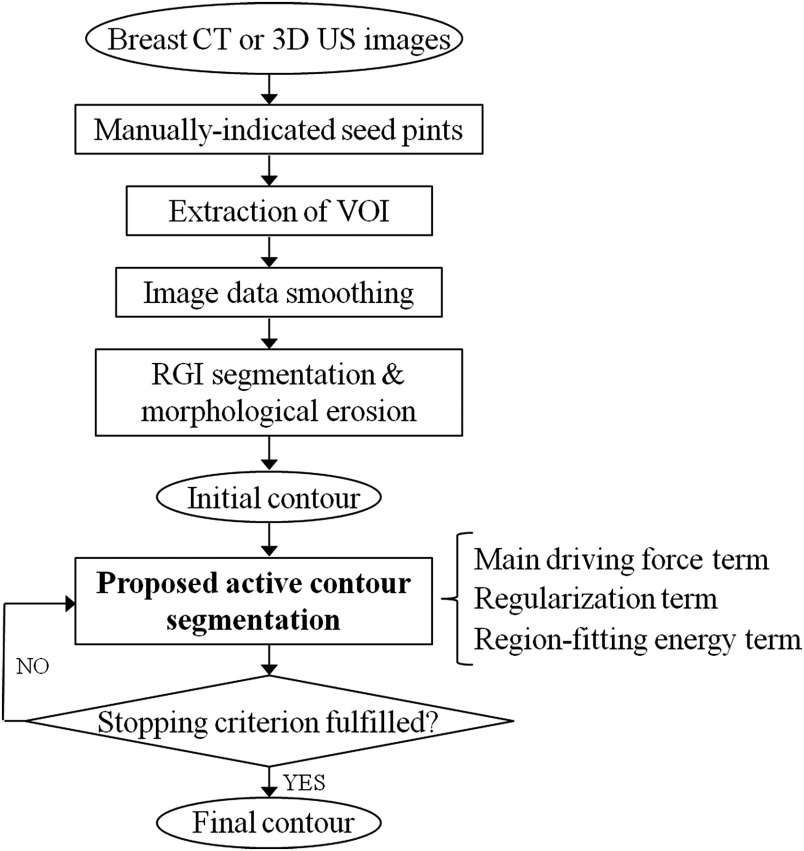
Our technique is a two-stage method that uses a RGI segmentation method^30,31 to first delineate the initial contour of the lesion and an active contour model to evolve the initial contour toward the lesion margins. As lesion margins are often ambiguous, we employ a dynamic stopping criterion²⁴ that is based on information of the surrounding region to terminate the segmentation procedure automatically. We evaluated the segmentation performance across the two modalities. Moreover, we also evaluated the relationship between the amount of existing breast fibroglandular tissues and the segmentation performance on bCT. This was conducted in order to investigate whether the proposed method would yield acceptable results when a lesion was surrounded by a large proportion of fibroglandular tissues, i.e., when a lesion was located in dense parenchyma. As an additional robustness analysis for 3-D ABUS, a comparison of segmentation performance on mammographically positive and mammographically occult lesions was conducted.

2. Materials

The bCT dataset included 35 breast volumes containing 38 contrast-enhanced masses (25 malignant and 13 benign) and 116 noncontrast breast volumes containing 129 masses (80 malignant and 49 benign) acquired at the University of California at Davis under an Institutional Review Board (IRB)-approved protocol. The coronal slice spacing varied from 200 to 400 μm. In coronal planes, the voxels were about $300{\mu \text{m}}^2$. Lesions were manually outlined in the coronal, sagittal, and axial planes by a research specialist (A.E.) with over 15 years of experience in mammography.

The ABUS images were acquired with a SomoVu system (U-Systems, a GE Health Care Company, Sunnyvale, California) at different clinical sites for a prior reader study¹⁰ under IRB-approved protocols. One should note that all patients who had ABUS in this study had breast imaging-reporting and data system breast density of 3 or 4, i.e., heterogeneously dense or extremely dense breasts. To ensure full coverage of all breast tissues with ABUS, each breast was imaged in three “views” (craniocaudal, mediolateral, and lateral), each yielding 3-D images and differing in transducer position and direction of compression. Generally, a mass is not visible in all views, and thus, the ABUS dataset included 98 images of 61 malignant masses from 52 patients. Of these 61 breast cancers, 32 were mammographically occult at the original clinical interpretation, and 29 were mammographically visible. Spatial resolution in the images was nonisotropic with spatial resolution in the axial plane of $\sim 250$ to 300 μm by $\sim 150\mu \text{m}$ and slice spacing of $\sim 600\mu \text{m}$. Lesion locations had been previously indicated for a prior reader study.¹⁰ In order to facilitate our evaluations, lesions were manually outlined by an expert breast radiologist with experience in breast ultrasound (C.A.S.).

3. Segmentation Methods

Our segmentation technique includes two stages—a contour initialization stage including a RGI segmentation method^30,31 that yields the initial contour of the lesion and an active contour model stage that evolves the initial contour toward the lesion margins (Fig. 1).

Fig. 1.

Flowchart of the 3-D automated breast lesion segmentation method.

3.1. Contour Initialization

Lesion boundaries in medical images can be complicated, and therefore, it is not guaranteed that the corresponding energy function is a simple convex function during the contour evolution process. Subsequently, an erroneous lesion contour might result due to local minima conditions. For this reason, we chose to initialize the active contour evolution with an approximate initial contour using RGI segmentation.^30,31

RGI segmentation, which has been extensively reported, is a seeded lesion segmentation method in which the determined lesion margin corresponds to the contour that maximizes the average proportion of gradients pointing radially outward from the lesion center.^30,31 In addition, to ensure that the initial approximation of the lesion contour is entirely inside the actual lesion, morphological erosion is performed with an adaptive cubic structuring element, with a side length of $1/9$ of the cube root of the RGI-segmented lesion volume. We have found RGI segmentation combined with the erosion process to be a reliable and fast method to generate initial contours that serve as an input to the active contour model in order to speed up and increase the robustness of the contour evolution. Additional details can be found in Kuo et al.¹³

3.2. Active Contour Model with Local Energy Term

The associated energy function, ${\mathcal{E}}_{\text{global}}$, of the level-set active contour model in our previous work¹³ is given as

$${\mathcal{E}}_{\text{global}}=\underset{\phi }{\int }\nu gH(\phi )\mathrm{d}\mathbf{r}+\mu g_s·\frac{1}{2}\underset{\mathrm{\Omega }}{\int }{(|\nabla \phi |-1)}^2\mathrm{d}\mathbf{r},$$ (1)

where $\nu$ and $\mu$ are parameters that control the direction of evolving surface (negative for evolving outward and positive for inward) and the strength of the second term¹³ in Eq. (1) (regularization term³²), respectively; $\phi$ is the level-set function such that the evolving surface $S=\{\mathbf{r}|\phi (\mathbf{r})=0\}$; $\mathbf{r}$ is the location vector $(x,y,z)$; and $H$ is the Heaviside function

$$H_{\alpha }(x)=\frac{1}{\pi }\arctan \left(\frac{x}{\alpha }\right),$$ (2)

$\alpha$ is a parameter controlling the steepness of $H$. In Eq. (1), $g$ is the edge indicator function proposed by Caselles et al.¹⁸

$$g=\frac{1}{1+{|\nabla G_{\sigma 1}\otimes I|}^2},$$ (3)

where $G_{\sigma 1}$ is a Gaussian kernel convolved with the given image $I$; and $g_s$ is defined as¹³

$$g_s=\frac{1}{1+|\nabla G_{\sigma 1}\otimes I|}.$$ (4)

The first term in Eq. (1) is the main driving force term that expands the surface uniformly. The second term in Eq. (1) is the regularization term first introduced by Li et al.³² This term allows for expression of the evolving surface as a signed distance function without re-initialization, which is more efficient.

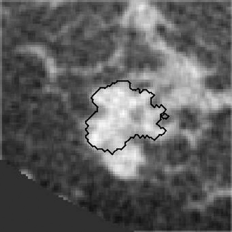
Malignant masses often have irregular shapes and present with vague lesion margins on breast CT (and other imaging modalities). Our previous model tended to yield a coarse outline, if a breast lesion lacked a clear margin (Fig. 2). To address this problem, we adapted Eq. (1) to have a region-fitting energy term, as originally proposed by Li et al.³⁵ The region-fitting energy term is based on the approximated intensities inside and outside the evolving surface in a local region. In general, the region-fitting energy function seeks optimal partitions of the lesion and background within the local region as determined by the size of a kernel mask, $G_{\sigma 2}$. The region fitting energy is defined as

$${\mathcal{E}}_{\text{local}}=\sum _{i=1}^2\int G_{\sigma 2}(\mathbf{a}-\mathbf{r}){|I(\mathbf{r})-f_i(\mathbf{a})|}^2{M}_i[\phi (\mathbf{r})]\mathrm{d}\mathbf{r},$$ (5)

where $G_{\sigma 2}$ is a Gaussian kernel with standard deviation $\sigma 2$, and $\mathbf{a}$ is the location of the kernel center. $M_1$ and $M_2$ are defined as [$H(\phi )+0.5$] and [$0.5-H(\phi )$], respectively, where $H$ is the Heaviside function given in Eq. (2), and $f_i$ are the approximated intensities inside and outside the local region (as explained in more detail in the Appendix).

Fig. 2.

The previous model can fail to segment lesions that are embedded in fibroglandular tissue or lesions with a complex shape. The figure shows a contour generated by our previous segmentation model.

By including Eq. (5) into Eq. (1), we introduce our new modified active contour model

$${\epsilon }_{\mathrm{snake}}={\epsilon }_{\text{global}}+{\epsilon }_{\text{local}}.$$ (6)

The Euler–Lagrange formulation corresponding to Eq. (6) is the level-set evolution equation used for segmenting breast masses in this study

$$\frac{\partial \phi }{\partial t}={\phi }^{k+1}-{\phi }^k=\tau \{\nu g{\delta }_{\alpha }(\phi )+\mu g_s[{\nabla }^2\phi -\mathrm{div}\left(\frac{\nabla \phi }{|\nabla \phi |}\right)\left]\right\}-{\delta }_{\alpha }(\phi )[\int G_{\sigma 2}(\mathbf{a}-\mathbf{r}){|I(\mathbf{r})-f_1(\mathbf{a})|}^2\mathrm{d}\mathbf{r}-\int G_{\sigma 2}(\mathbf{a}-\mathbf{r}){|I(\mathbf{r})-f_2(\mathbf{a})|}^2\mathrm{d}\mathbf{r}],$$ (7)

where $\tau$ is an iteration step constant. The derivation of Eq. (7) from Eq. (6) is presented in the Appendix. Throughout the remainder of this article, we will refer to Eq. (1) as our “previous model” and Eq. (6) as our “proposed model.”

3.3. Implementation

The parameter settings in this study are listed in Table 1. The selection of parameters follows our previous work.¹³ Based on Kuo et al.,¹³ the value of $\tau \mu$ was selected to be 0.1. Due to ultrasound images often lacking sharp edges, we used a smaller $\tau$ (100) for a smaller iteration step, and thus requiring $\mu$ to be 0.01.

Table 1.

Active contour model parameter values for segmentation of bCT and ABUS lesions.

	$\tau$	$\nu$	$\mu$	$\alpha$	Maximum number of iterations
bCT	1000	$-10$	0.001	0.2	300
ABUS	100	$-10$	0.01	0.2	300

See Eq. (6) for $\tau$, Eq. (1) for $\nu$ and $\mu$, and Eq. (2) for $\alpha$.

3.4. Dynamic Stopping Criterion

Because lesion margins are often ambiguous in medical images, it is necessary to use a stopping criterion for the active contour model. We adopted the dynamic stopping criterion proposed by Yuan et al.²⁴ The stopping criterion is defined as $(\mathrm{d}\overline{I_L}/\mathrm{d}t-\mathrm{d}\overline{I_B}/\mathrm{d}t)=0$, where $\overline{I_L}$ is the mean intensity within the segmented region, $\overline{I_B}$ is the mean intensity outside the segmented region, and $t$ refers to iteration. When $(\mathrm{d}\overline{I_L}/\mathrm{d}t-\mathrm{d}\overline{I_B}/\mathrm{d}t)\approx 0$, the evolving contour is on the margin of foreground and background, and thus the contour evolution is terminated.

4. Segmentation Evaluation

4.1. Segmentation Performance in Terms of DICE

Due to the large number of slices contained in each image volume, our expert was only able to outline each lesion in the three central orthogonal planes throughout the database. Therefore, computer-segmented margins were evaluated on these three orthogonal slices through the lesion center in comparison to the manually delineated lesions. Segmentation performance was presented in terms of the DICE, an overlap measure between the manually delineated margins and computer-segmented margins on the three orthogonal slices

$$\mathrm{DICE}=\frac{1}{3}\{{\left[\frac{2(\mathrm{\Omega }\cap {\omega }_{\text{man}})}{\mathrm{\Omega }+{\omega }_{\text{man}}}\right]}_{xy}+{\left[\frac{2(\mathrm{\Omega }\cap {\omega }_{\mathrm{man}})}{\mathrm{\Omega }+{\omega }_{\mathrm{man}}}\right]}_{yz}+{\left[\frac{2(\mathrm{\Omega }\cap {\omega }_{\mathrm{man}})}{\mathrm{\Omega }+{\omega }_{\mathrm{man}}}\right]}_{xz}\},$$ (8)

where $\mathrm{\Omega }$ is the computer segmentation, and ($xy$), ($yz$), and ($xz$) denote the orientations of each slice through the lesion center. ${\omega }_{\text{man}}$ is the human-delineated lesion margin in the same orthogonal slice. Note that the DICE value for a given lesion is the average of the DICE values over the three orthogonal planes. According to Zijdenbos et al.,³³ a $\mathrm{DICE}\ge 0.7$ indicates “good” overlap between computer and human outlines for medical images.

We compared the segmentation performance between the previous model [Eq. (1)] and the proposed model [Eq. (6)]. Statistical significance of differences in performance was assessed using paired t-tests of DICE.

4.2. Segmentation Performance and Presence of Fibroglandular Tissue on bCT

Since fibroglandular tissue has an x-ray attenuation coefficient similar to that of tumor tissue, the presence of fibroglandular tissue adjacent to a lesion poses challenges for segmentation. To investigate the dependence of lesion segmentation quality on the presence of fibroglandular tissue in the immediate vicinity of lesions, we used a fuzzy c-means-based segmentation scheme to identify fibroglandular tissue.³⁶ The proportion of fibroglandular tissue in a lesion’s vicinity was calculated from a $50\times 50\text{-}{\mathrm{mm}}^2$ region on each of the three orthogonal central slices, on which the manual lesion delineations were performed, and was defined as the area of the fibroglandular tissue (as identified by the fuzzy c-means method) relative to the area of the three slices excluding the manually outlined lesion area. Based on the work of Yaffe et al.,³⁷ 95% of women have breast density of lower than 45% when imaged with bCT with mean glandular fraction of 19.3%. Therefore, for our local density categorization, we used 20% and 40% as thresholds to divide our database into three categories ($\le 20\%$, 20% to 40%, and $\ge 40\%$).

4.3. ABUS Segmentation Performance on Mammographically Occult and Mammographically Positive Breast Cancers

We assessed segmentation performance for all ABUS-imaged lesions and investigated whether there were any differences in performance between lesions that were occult on mammography and those that were visible on mammography. Note that all lesions in this 3-D US dataset were malignant. Since US is known for its ability to detect mammographically occult cancers and has recently been approved in the United States as an adjunct screening modality for women with dense breasts, it is important to assess the performance of our segmentation methods for mammographically negative and mammographically positive lesions separately.

5. Results

5.1. Impact of the New Modifications to the Active Contour Method: an Example

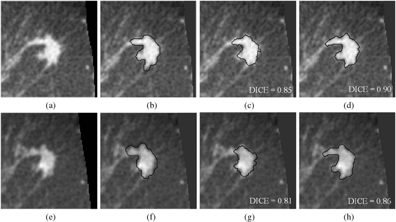
In this study, a new term ${\mathcal{E}}_{\text{local}}$ [see Eq. (5)] was added to the original active contour model. To illustrate the impact of this term, Fig. 3 shows both contrast-enhanced and noncontrast breast CT images, manual delineations, and computer-determined segmentations (using our previous and proposed methods) of a lesion with a complicated shape.

Fig. 3.

(a–d) Noncontrast-enhanced images. (e–h) Contrast-enhanced images. (b and f) Research specialist’s outlines. (c and g) Segmentations by our previous model. (d and h) Segmentations by the proposed model. Note that these eight images are of the same patient (case), and they are displayed in the central coronal plane through the lesion seed point. For this case, the proportion of fibroglandular tissue is 12%.

For this example, the DICE values of our previous segmentation model were satisfactory, but were improved by including the new term ${\mathcal{E}}_{\text{local}}$ in the segmentation model for both contrast and noncontrast images. As this example illustrates, the proposed segmentation method was able to capture more shape detail.

5.2. Comparison of Previous and Proposed Segmentation Models

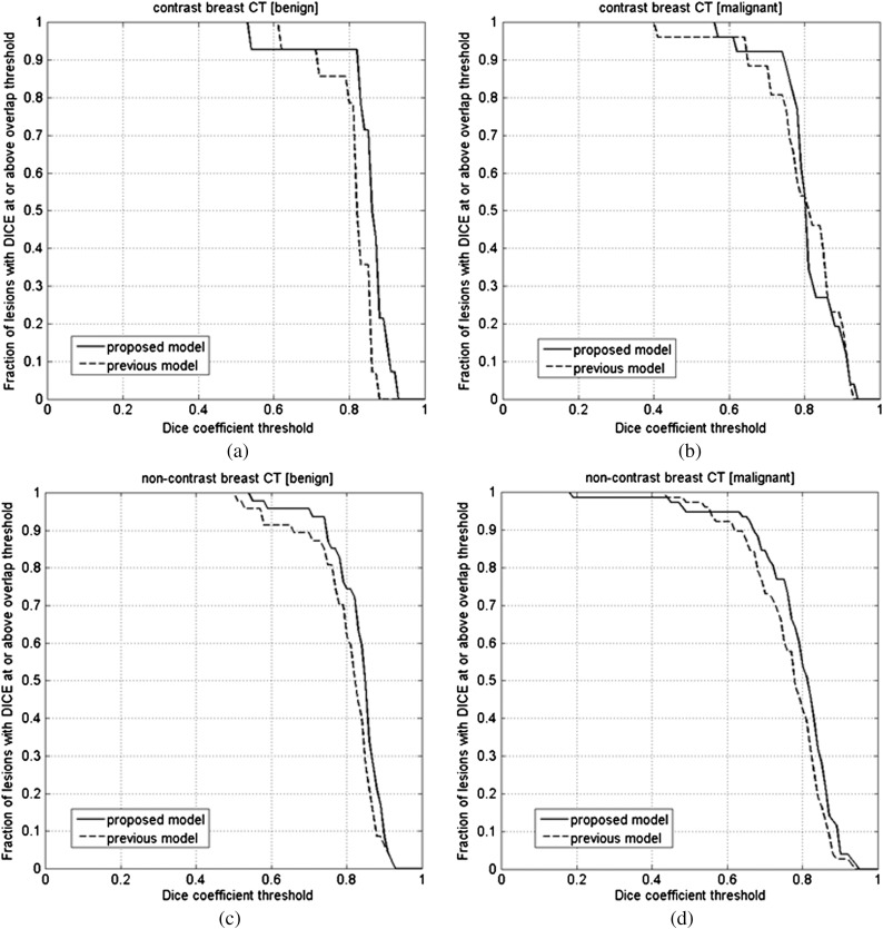
We compared the proposed segmentation model, Eq. (6), to our previous model, Eq. (1) (Tables 2 and 3). For the noncontrast bCT images, the proposed segmentation model obtained significantly better segmentation with respect to our previous model ($p\ll 0.05$) for both malignant and benign lesions (Table 2). It appeared to slightly improve the performance for contrast bCT, but this improvement failed to reach statistical significance ($p=0.30$). For the 3-D ABUS dataset (Table 3), both models segmented the lesions well. Figures 4 and 5 show the fraction of lesions correctly segmented at various overlap (DICE) thresholds in bCT and 3-D ABUS, with several segmentation examples shown in Figs. 7–9.

Table 2.

Segmentation results for contrast-enhanced and noncontrast-enhanced bCT.

		Segmentation model	Performance in DICE ($\text{mean}\pm \mathrm{std}$)	Percentage of $\ge 0.7$ DICE (%)	$p$-value of paired t-test between the two models
Contrast-enhanced bCT	Benign cases ($N=13$)	Previous model	$0.81\pm 0.07$	93	0.24
		Proposed model	$0.84\pm 0.09$	93
	Malignant cases ($N=25$)	Previous model	$0.80\pm 0.11$	88	0.65
		Proposed model	$0.81\pm 0.08$	92
	All cases ($N=38$)	Previous model	$0.80\pm 0.10$	90	0.30
		Proposed model	$0.82\pm 0.10$	93
Noncontrast bCT	Benign cases ($N=49$)	Previous model	$0.80\pm 0.10$	89	0.005
		Proposed model	$0.83\pm 0.08$	96
	Malignant cases ($N=80$)	Previous Model	$0.76\pm 0.10$	73	0.04
		Proposed model	$0.78\pm 0.12$	85
	All cases ($N=129$)	Previous model	$0.77\pm 0.10$	79	0.0016
		Proposed model	$0.80\pm 0.11$	89

Table 3.

Segmentation results for 3-D breast ultrasound.

	Average size (mm)	Segmentation model	Performance in DICE ($\mathrm{mean}\pm \mathrm{std}$)	Percentage of $\ge 0.7$ DICE (%)	$p$-value of paired t-test between the two models
Mammographically occult ($N=54$)	$16.79\pm 13.20$	Previous model	$0.73\pm 0.15$	77	0.57
		Proposed model	$0.72\pm 0.18$	71
Mommographically positive ($N=44$)	$19.41\pm 12.31$	Previous model	$0.69\pm 0.15$	61	0.57
		Proposed model	$0.71\pm 0.13$	63
All images ($N=98$)	$17.97\pm 12.80$	Previous model	$0.72\pm 0.13$	70	0.93
		Proposed model	$0.71\pm 0.16$	68

Fig. 4.

(a) The comparison of segmentation between the proposed and previous segmentation methods on the contrast bCT benign dataset ($N=13$). (b) The comparison of segmentation between the proposed and previous segmentations on the contrast bCT malignant dataset ($N=25$). (c) The comparison of segmentation between the proposed and previous segmentations on the noncontrast bCT benign dataset ($N=49$). (d) The comparison of segmentation between the proposed and previous segmentations on the noncontrast bCT malignant dataset ($N=80$).

Fig. 5.

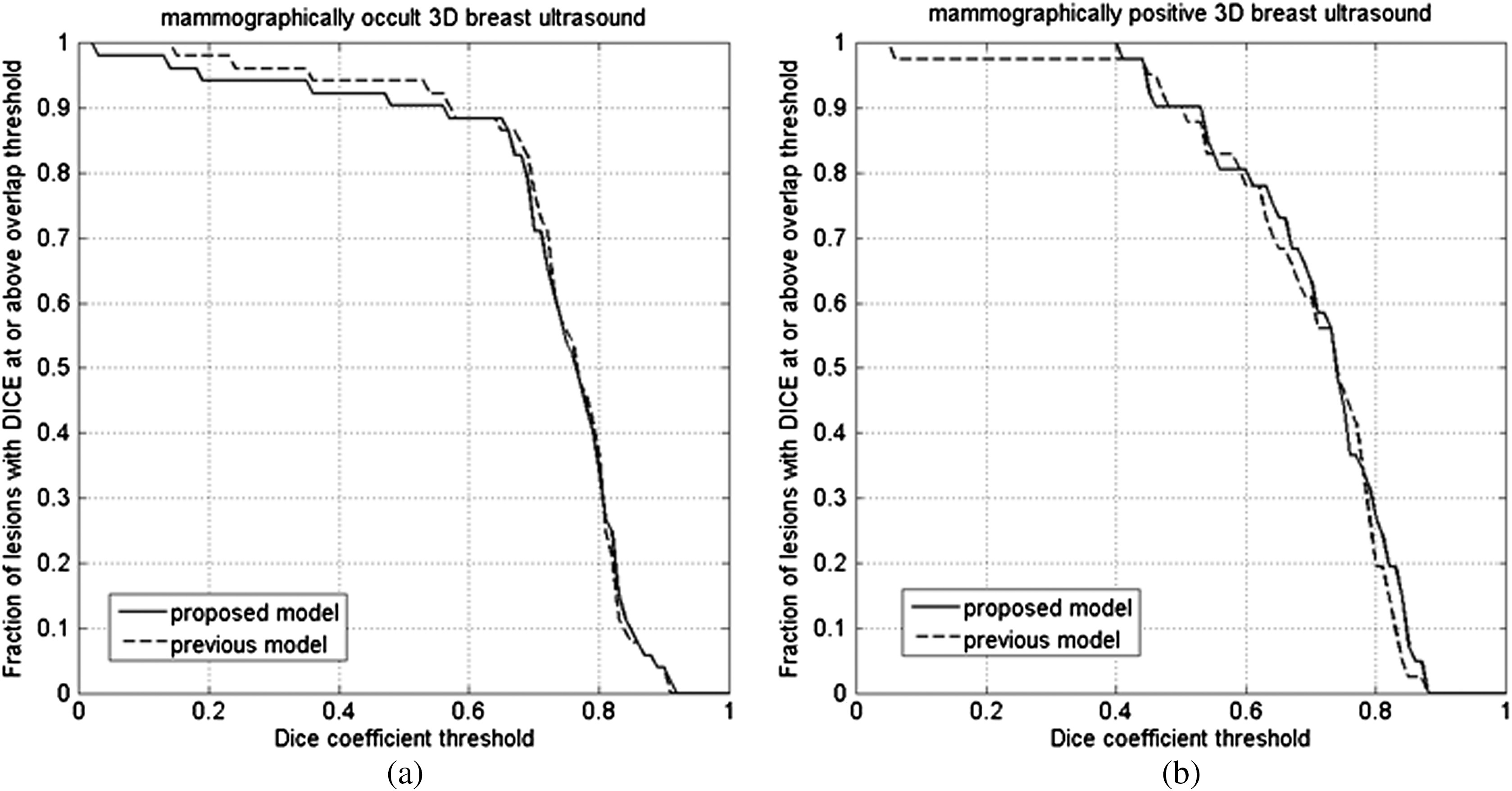
Segmentation performance in (a) 54 mammographically occult and (b) 44 mammographically positive 3-D breast US images.

Fig. 7.

A contrast-enhanced bCT image example. (a) Original volume of interest. (b) Research specialist’s outline. (c) Segmentation result by using previous procedure. (d) Segmentation result by using proposed procedure. The proportion of fibroglandular tissue in the lesion vicinity is 29%.

Fig. 8.

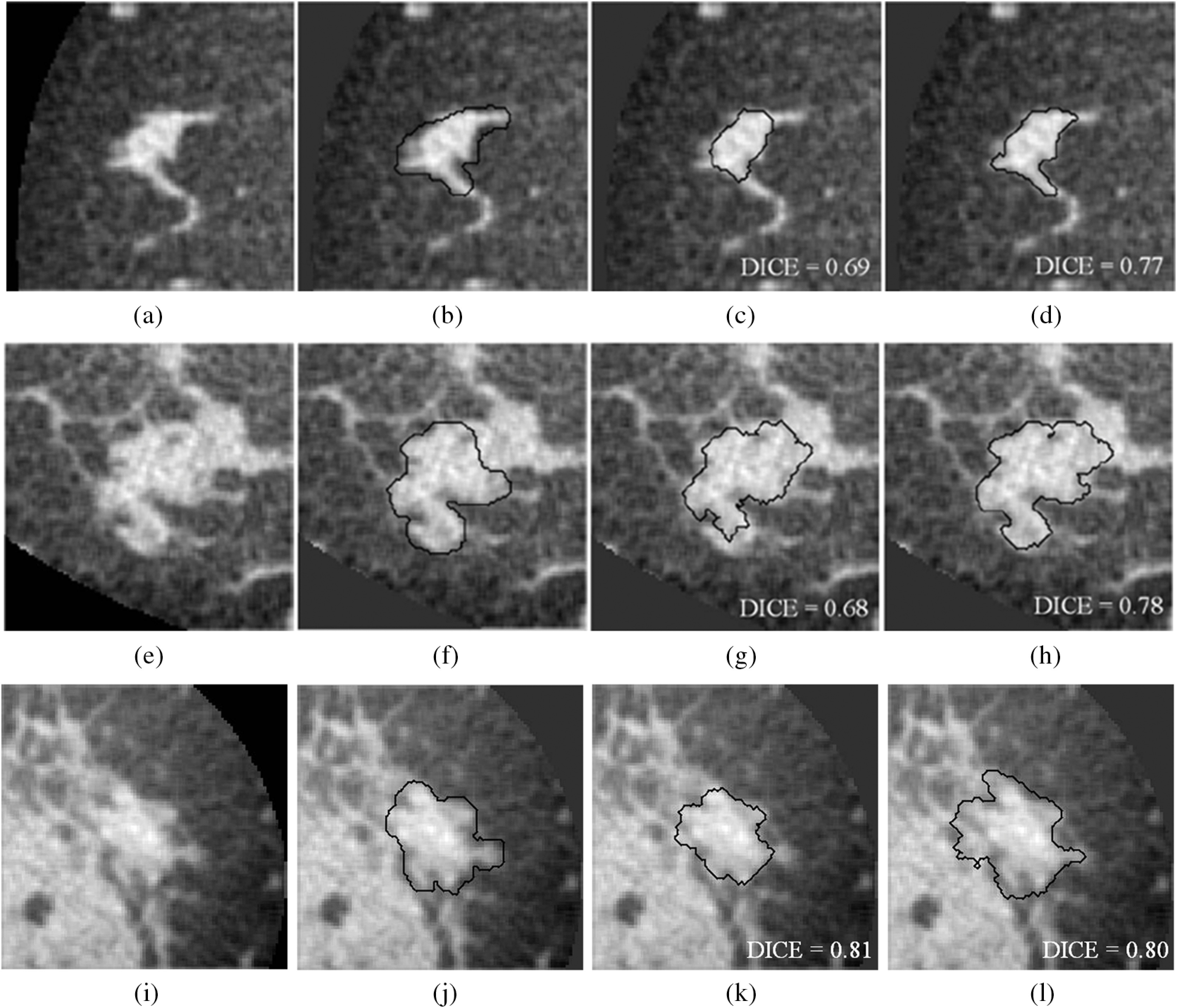
Three different noncontrast bCT segmentation examples for each of the fibroglandular density classes. (a–d) 8% of fibroglandular proportion (low density). (e–h) 29% fibroglandular proportion (intermediate density; this lesion is also depicted in Fig. 7). (i–l) 46% fibroglandular proportion (high density). (b, f, and j) Research specialist’s outlines. (c, g, and k) Segmentation results by previous procedure. (d, h, and l) Segmentation results by proposed procedure.

Fig. 9.

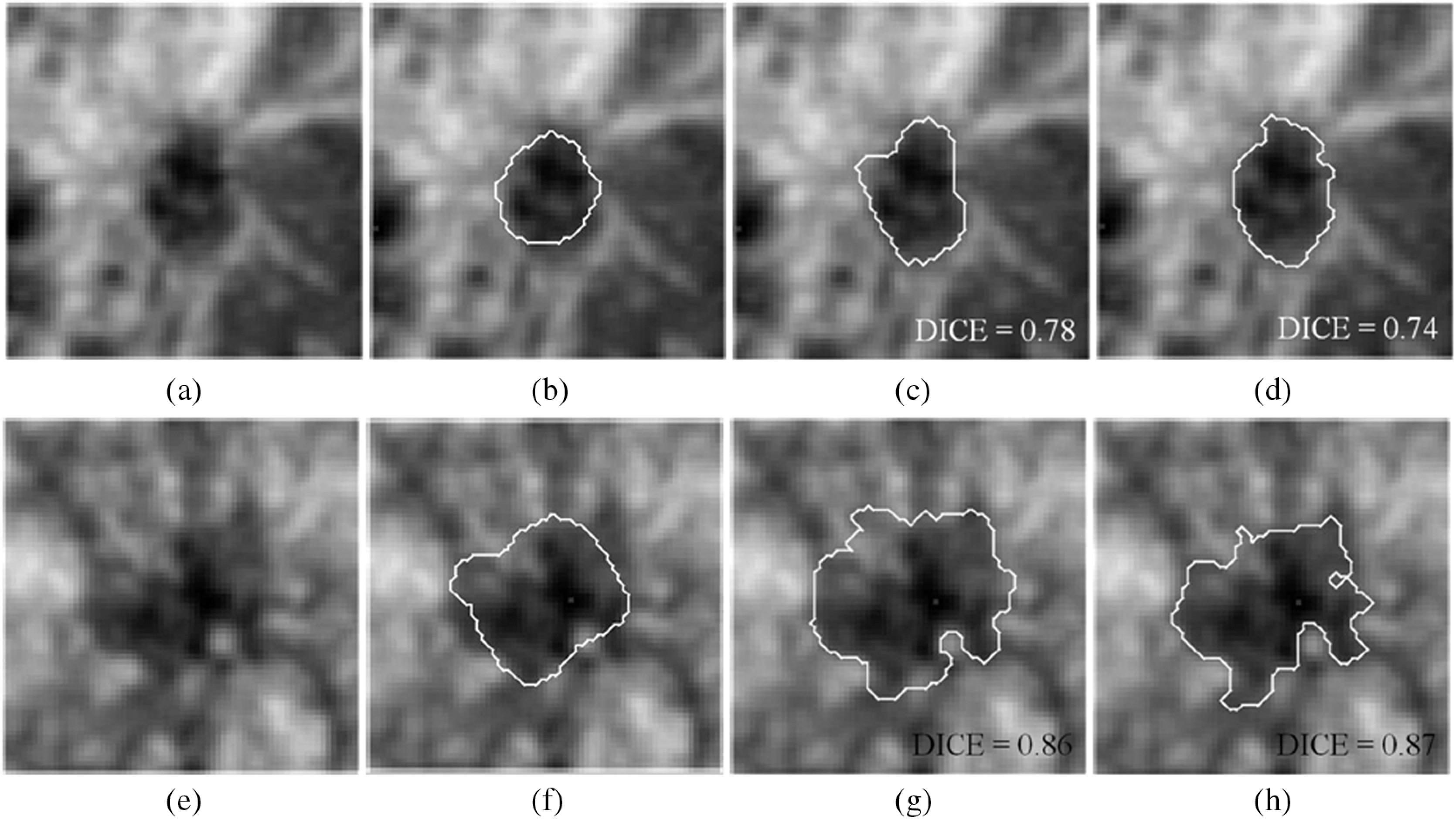
Two examples of 3-D breast ultrasound segmentation on two cancerous lesions. (a–d) Mammographically occult example. (e–h) Mammographically positive example. (b and f) Medical doctor’s outlines. (c and g) Segmentation results by previous procedure. (d and h) Segmentation results by proposed procedure. Unlike traditional ultrasound images displaying in axial or sagittal plane, the images shown in this figure are displayed in coronal plane.

5.3. Segmentation Performance and Presenting Fibroglandular Tissue

The relationship between the segmentation performance and the proportion of fibroglandular tissue in the lesion vicinity on bCT images is shown in Fig. 6 and Table 4. For noncontrast bCT, the segmentation performance decreases when the proportion of fibroglandular tissue exceeds 40%, but the DICE is still above 0.7. Segmentation examples for different “local fibro-density classes” are shown in Fig. 8.

Fig. 6.

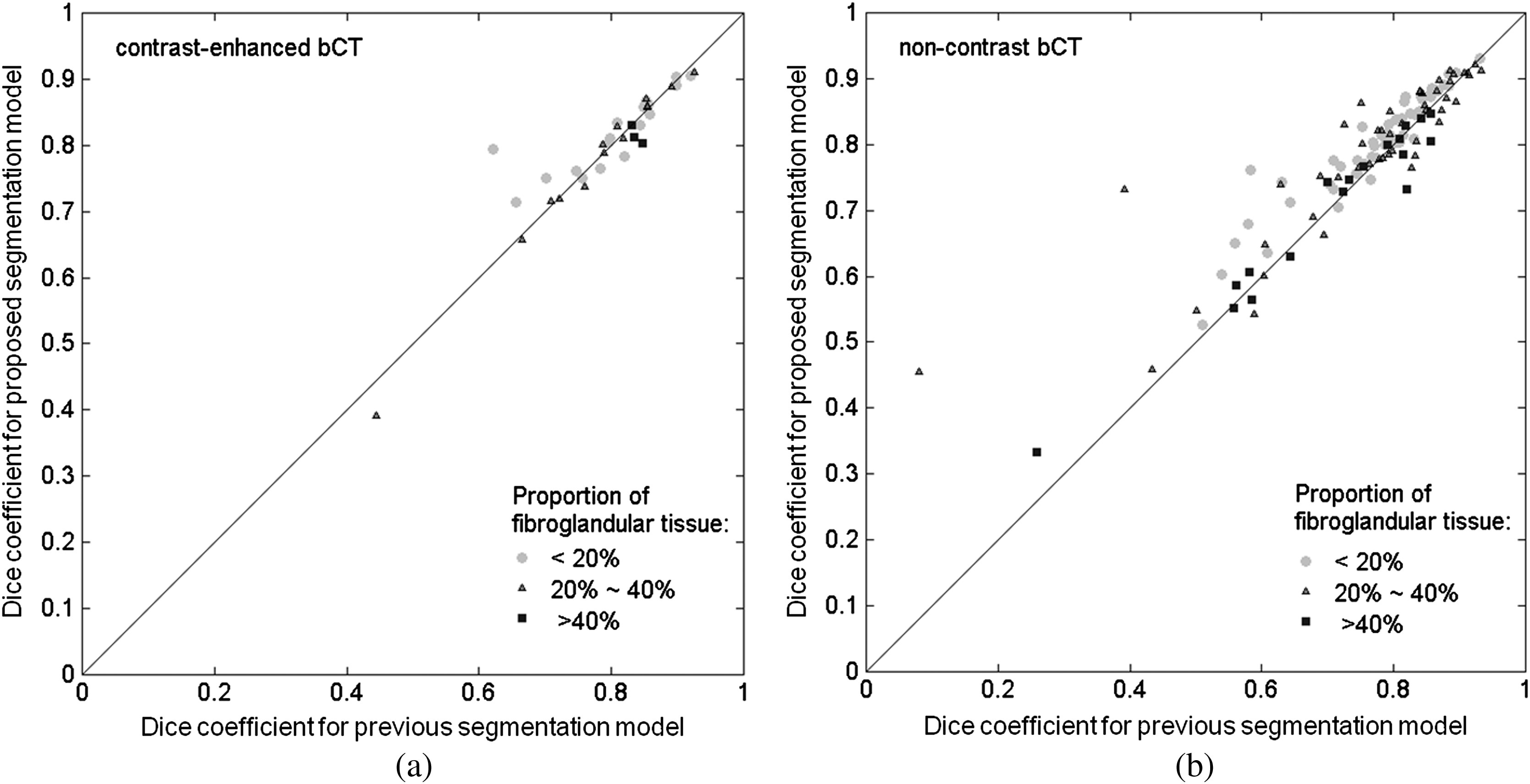
Comparison of lesion DICE value for the previous and proposed segmentation models for (a) the contrast-enhanced and (b) noncontrast bCT datasets across different fibroglandular density categories.

Table 4.

Segmentation performance on bCT across different fibroglandular density categories.

Proportion of fibroglandular tissue in lesion neighborhood		$<20\%$		20% to 40%		$>40\%$
		$\mathrm{DICE}\pm \mathrm{std}$	Paired t-test $p$-value	$\mathrm{DICE}\pm \mathrm{std}$	Paired t-test $p$-value	$\mathrm{DICE}\pm \mathrm{std}$	Paired t-test $p$-value
Contrast-enhanced bCT	Previous model	$0.81\pm 0.08$	0.15 ($N=20$)	$0.78\pm 0.12$	0.57 ($N=15$)	$0.84\pm 0.01$	0.23 ($N=3$)
	Proposed model	$0.82\pm 0.06$		$0.77\pm 0.13$		$0.82\pm 0.01$
Noncontrast bCT	Previous model	$0.77\pm 0.09$	$\ll 0.05$ ($N=56$)	$0.77\pm 0.16$	0.01 ($N=55$)	$0.71\pm 0.15$	0.98 ($N=18$)
	Proposed model	$0.80\pm 0.08$		$0.79\pm 0.12$		$0.71\pm 0.14$

5.4. ABUS Segmentation Performance for Mammographically Occult and Mammographically Positive Breast Cancer

Both our previous segmentation model and the proposed model performed well for both mammographically occult and mammographically positive breast cancers (Fig. 5 and Table 3). There was no statistically significant difference (Table 3) between the two segmentation methods within each ABUS image category. However, overall, the performance appeared to be slightly better for mammographically occult lesions than for mammographically positive lesions for both segmentation procedures on the ABUS images. Two segmentation examples are shown in Fig. 9.

6. Discussion and Conclusion

In this study, we modified our previous two-stage 3-D lesion segmentation algorithm to allow for the inclusion of more shape detail. The region-fitting energy term, which was introduced in the new model, not only improved the delineation of shape detail, but also helped smooth the lesion contour and correct the contour evolution, if the main driving term caused inaccuracies.

The proposed model showed statistically improved segmentation performance for the noncontrast bCT images ($p\ll 0.05$). The previous model often missed shape details when a lesion presented with a complex margin [e.g., Figs. 7(c) and 8(g)]. The improved ability to capture shape and margin characteristics should be useful clinically, since such morphological information plays an important role in diagnosis.^38–43 Improvement in diagnosis on noncontrast bCT images is important, since contrast-enhanced bCT requires the placement of an intravenous and carries a risk of allergic reaction. Hence, the improved ability of the proposed method to capture shape details may have an impact on future implementations in CAD and allow for more accurate lesion classification. The proposed segmentation model failed to yield significant improvement over our previous segmentation model on contrast-enhanced bCT images, likely because the conspicuity of cancers is significantly higher on contrast-enhanced bCT (Prionas et al.⁷) and reasonable segmentation performance with our prior methods was facilitated by this conspicuity.

The computation time varied from case to case, depending on the size of the lesion. The proposed segmentation model requires a longer time for the segmentation process as compared with the previous model, since an additional local energy term is included. In Figs. 8(d) and 8(l), it took 208.8 and 710.9 s to reach the final contour, respectively. In general, segmentation process is faster in ABUS than in bCT due to a smaller number of voxels contained in each ABUS image volume. In Figs. 9(d) and 9(h), it took 174.7 and 225.7 s, respectively.

Breast density is a risk factor for breast cancer,^41–43 and the masking effect of dense tissue reduces the sensitivity of imaging modalities in breast cancer diagnosis. Therefore, it is important to successfully segment lesions within dense tissue. In contrast-enhanced bCT, the segmentation performance appeared to decrease with higher volume glandular fraction (Table 4). However, the DICE for higher density ($>40\%$) breasts is still above 0.75 (Table 4, note that there are only three cases in the high-density class for contrast-enhanced bCT). In noncontrast bCT, the segmentation performance was affected when the proportion of fibroglandular tissues was high, but the DICE was still above 0.7 for both segmentation models (Table 4). According to Table 4, there is not much improvement for the $>40\%$ category. Due to the similar x-ray attenuation of tumor masses and fibroglandular tissues, the proposed segmentation model could yield slightly oversegmented results and leads to a decrease in DICE, since the proposed model possesses better ability to capture edge details [Figs. 8(i)–8(l)]. Overall, both segmentation models behaved similarly with respect to the volume glandular fraction.

For 3-D breast ultrasound, our results showed similar good performance for the previous and proposed segmentation models (Table 3). The presence of ultrasound speckle and anisotropic image resolution may be the cause of the lack of improvement. It should be noted, however, that the performance of both models was quite satisfactory, demonstrating the robustness of our segmentation methods across 3-D imaging modalities since they were initially developed for bCT, and that ultrasound-specific preprocessing or model refinements could potentially further improve segmentation.

Limitations to this study include that for each imaging modality, only a single expert outlined the lesions which defined the reference standard for segmentation. In future studies, we will investigate how the different segmentation methods affect computerized lesion characterization and classification for malignancy. Furthermore, we did not attempt to optimize our methods for the ABUS images, and further ultrasound-modality–specific improvements to the model may be possible. On the other hand, it is important to note that the current study demonstrated robustness across different 3D imaging modalities, holding promise for potential future application to other 3D breast images.

To conclude, we presented a 3-D segmentation method adapted and refined from our previous model developed for contrast-enhanced breast CT¹³ and evaluated the methods across two emerging 3-D breast imaging modalities—dedicated breast CT (both contrast-enhanced and noncontrast bCTs) and ABUS. We obtained promising results that warrant future implementation within computer-aided diagnosis software platforms and quantitative imaging.

Biographies

Hsien-Chi Kuo received a PhD in biomedical engineering in 2013. He joined Dr. Maryellen L. Giger’s lab at the University of Chicago working on the areas of computer-aided diagnosis and quantitative image analysis from 2010 to present. He has been active in breast tumor segmentation in bCT, 3-D breast ultrasound, and breast MRI images. His research interest also includes tumor classification by utilizing pattern recognition techniques.

Maryellen L. Giger is the A. N. Pritzker professor of radiology/medical physics at the University of Chicago in Chicago, Illinois. She has a PhD in medical physics from the University of Chicago. She works in the areas of computer-aided diagnosis and quantitative image analysis with a focus on novel methods for characterizing breast cancer on mammography, bCT, ultrasound, and MRI. She has published over 180 peer-reviewed papers, and her research presented here has been funded by the National Institutes of Health (NCI and NIBIB).

Ingrid Reiser is assistant professor of radiology at the University of Chicago in Chicago, Illinois. She holds a PhD in physics from Kansas State University. Her research interests include computer-aided detection and diagnosis methods for breast cancer in dedicated breast CT and digital breast tomosynthesis, as well as objective assessment of x-ray tomographic x-ray breast imaging systems.

Karen Drukker, PhD, has been active in breast image analysis research at the University of Chicago for over a decade. Interests include computer-aided diagnosis and detection for mammography, hand-held ultrasound, 3-D automated whole breast ultrasound, breast MRI, and dedicated breast CT.

John M. Boone is professor and vice chair (Research) of radiology, and professor of biomedical engineering at University of California Davis. After receiving a BA in biophysics from UC Berkeley, he received a PhD in radiological sciences from UC Irvine. He has research interests in breast imaging, CT, and radiation dosimetry; he is the PI of the breast tomography project, where over 600 women have been imaged on breast CT scanners fabricated in his laboratory.

Karen K. Lindfors is a professor of radiology and the Chief of Breast Imaging at the University of California, Davis School of Medicine. She has an MD from the University of Louisville and an MPH from Yale University. She completed her diagnostic radiology residency and fellowship in oncologic imaging at the Massachusetts General Hospital. She has published over 75 scientific papers. Her current research centers around the development and assessment of dedicated breast computed tomography.

Kai Yang is an assistant adjunct professor of radiology at University of California, Davis. He has a PhD in biomedical engineering from University of California, Davis. He works in the areas of dedicated computed tomography imaging with the focus on bCT for breast cancer detection and micro-CT for surgical specimen imaging. He has published over 25 peer-reviewed papers, and his research presented here has been funded by the National Institutes of Health (NIBIB).

Biographies of the other authors are not available.

Appendix.

In the appendix, we provide the derivation of the level-set evolution function [Eq. (7)] from Eq. (6). We start with the need to determine the level-set function $\phi$ that minimizes the energy function by $\mathrm{d}{\mathcal{E}}_{\text{snake}}/\mathrm{d}\phi =0$. In Eq. (6), the energy function combines a main driving term [the first term in Eq. (1)], a regularization term [the second term in Eq. (1)], and a region-fitting energy term [Eq. (5)]. For convenience, we denote the main driving term as $A$, the regularization term as $B$, and the region-fitting energy term as $C$. To derive Eq. (7) from Eq. (6), one needs to compute the associated Euler–Lagrange equation [Eq. (6)] using the first variation of calculus.⁴⁴ The minimum of Eq. (6) occurs when the following condition is satisfied:

$$\frac{\mathrm{d}}{\mathrm{d}x}\left[\frac{\partial (A+B+C)}{\partial {\phi }_x}\right]+\frac{\mathrm{d}}{\mathrm{d}y}\left[\frac{\partial (A+B+C)}{\partial {\phi }_y}\right]+\frac{\mathrm{d}}{\mathrm{d}z}\left[\frac{\partial (A+B+C)}{\partial {\phi }_z}\right]-\frac{\partial (A+B+C)}{\partial \phi }=0.$$ (9)

We address $A$, $B$, and $C$ separately. For term $A$

$$\frac{\mathrm{d}}{\mathrm{d}x}\frac{\partial \nu g{H}_{\alpha }(\phi )}{\partial {\phi }_x}+\frac{\mathrm{d}}{\mathrm{d}y}\frac{\partial \nu g{H}_{\alpha }(\phi )}{\partial {\phi }_y}+\frac{\mathrm{d}}{\mathrm{d}z}\frac{\partial \nu g{H}_{\alpha }(\phi )}{\partial {\phi }_z}-\frac{\partial \nu g{H}_{\alpha }(\phi )}{\partial \phi }=\nu g{H_{\alpha }}^{\prime }(\phi )=\nu g{\delta }_{\alpha }(\phi ),$$ (10)

where ${\delta }_{\alpha }$ is the derivative of $H_{\alpha }$ with respect to $\phi$

$${\delta }_{\alpha }=\frac{1}{\pi }·\frac{\alpha }{{\alpha }^2+x^2}.$$ (11)

For term $B$, the partial derivative of $\partial B/\partial {\phi }_x$ with respect to $x$ is given as:

$$\frac{\mathrm{d}}{\mathrm{d}x}\frac{\partial \mu g_s\left[\frac{1}{2}{(|\nabla \phi |-1)}^2\right]}{\partial {\phi }_x}=\mu g_s\frac{\mathrm{d}}{\mathrm{d}x}({\phi }_x-\frac{{\phi }_x}{\Vert \nabla \phi \Vert }),$$ (12)

and the partial derivative of $\partial B/\partial {\phi }_y$ with respect to $y$ and the partial derivative of $\partial B/\partial {\phi }_z$ with respect to $z$ are similarly derived. Given

$$\frac{\partial \mu g_s\left[\frac{1}{2}{(|\nabla \phi |-1)}^2\right]}{\partial \phi }=0,$$ (13)

we have

$$\mu g_s\left[\frac{\mathrm{d}}{\mathrm{d}x}\right({\phi }_x-\frac{{\phi }_x}{\nabla \phi })+\frac{\mathrm{d}}{\mathrm{d}y}({\phi }_y-\frac{{\phi }_y}{\nabla \phi })+\frac{\mathrm{d}}{\mathrm{d}z}({\phi }_z-\frac{{\phi }_z}{\nabla \phi }\left)\right]=\mu g_s[{\nabla }^2\phi -\mathrm{div}(\frac{\nabla \phi }{|\nabla \phi |}\left)\right].$$ (14)

For term $C$, we employ the steepest descent method⁴⁵ to derive the associated Euler–Lagrange equation. By fixing the approximated intensities $f_1(\mathbf{a})$ and $f_2(\mathbf{a})$, the minimum of the region-fitting energy term $C$ occurs when

$$-{\delta }_{\alpha }(\phi )({\lambda }_1{a}_1-{\lambda }_2{a}_2)=0,$$ (15)

where

$$a_i={\lambda }_1\int G_{\sigma 2}(\mathbf{a}-\mathbf{r}){|I(\mathbf{r})-f_1(\mathbf{a})|}^2\mathrm{d}\mathbf{r},i=1,2\dots$$ (16)

Using steepest descent method, assembling Eqs. (10), (14), and (16), we reach the level-set formulation of the contour evolution function Eq. (7) with an added time-step constant $\tau$ on the first two terms.

Now, we give the derivation of the approximated intensities $a_1$ and $a_2$. It is also obtained by using the steepest descent method to minimize the region-fitting energy function with the level-set function $\phi$ fixed. Given this condition, one can find the minimum of the energy function $C$ with respect to $f_1(a)$ and $f_2(a)$ when the following satisfies:

$$\int G_{\sigma 2}(\mathbf{r}-\mathbf{a})M_i[\phi (\mathbf{r})]|I(\mathbf{r})-f_i(\mathbf{a})|\mathrm{d}\mathbf{r}=0,i=1,2\dots ,$$ (17)

From Eq. (17), we can obtain $f_i(a)$ as

$$f_i(\mathbf{a})=\frac{G_{\sigma 2}(\mathbf{a})\otimes [M_i(\phi (\mathbf{r})]I(\mathbf{r}))}{G_{\sigma 2}(\mathbf{a})\otimes M_i[\phi (\mathbf{r})]},i=1,2.$$ (18)

References

- 1.Lindfors K. K., et al. , “Dedicated breast computed tomography: the optimal cross-sectional imaging solution?” Radiology 48(5), 1043–1054 (2010). 10.1016/j.rcl.2010.06.001 [DOI] [PMC free article] [PubMed] [Google Scholar]
- 2.Glick S. J., “Breast CT,” Annu. Rev. Biomed. Eng. 9, 501–526 (2007). 10.1146/annurev.bioeng.9.060906.151924 [DOI] [PubMed] [Google Scholar]
- 3.Dershaw D. D., “Breast disease missed by mammography,” Appl. Radiol. 26(9), 24–28 (1997). 10.1016/S0160-9963(00)80025-4 [DOI] [Google Scholar]
- 4.Huynb P. T., Jarolimek A. M., Daye A., “The false-negative mammogram,” Radiographics 18, 1137–1154 (1998). 10.1148/radiographics.18.5.9747612 [DOI] [PubMed] [Google Scholar]
- 5.Kalender W. A., et al. , “High-resolution spiral CT of the breast at very low dose: concept and feasibility considerations,” Eur. Radiol. 22(1), 1–8 (2012). 10.1007/s00330-011-2169-4 [DOI] [PubMed] [Google Scholar]
- 6.Lindfors K. K., et al. , “Dedicated breast CT: initial clinical experience,” Radiology 246(3), 725–733 (2008). 10.1148/radiol.2463070410 [DOI] [PMC free article] [PubMed] [Google Scholar]
- 7.Prionas N. D., et al. , “Contrast-enhanced dedicated breast CT: initial clinical experience,” Radiology 256(3), 714–723 (2010). 10.1148/radiol.10092311 [DOI] [PMC free article] [PubMed] [Google Scholar]
- 8.Chou Y., et al. , “Automated full-field breast ultrasonography: the past and the present,” J. Med. Ultrasound 15(1), 31–44 (2007). 10.1016/S0929-6441(08)60022-3 [DOI] [Google Scholar]
- 9.Kolb T. M., Lichy J., Newhouse J. H., “Occult cancer in women with dense breasts: detection with screening US—diagnosis yield and tumor characteristics,” Radiology 207(1), 191–199 (1998). [DOI] [PubMed] [Google Scholar]
- 10.Giger M. L., et al. , “Clinical reader study examining the performance of mammography and automatic breast ultrasound in breast cancer screening,” in The 2012 Annual Meeting of Radiological Society of North America (RSNA), Chicago, IL, Paper SSJ01–04. [Google Scholar]
- 11.Kolb T. M., Lichy J., Newhouse J. H., “Comparison of the performance of screening mammography, physical, examination, and breast US and evaluation of factors that influence them: an analysis of 27,825 patient evaluations,” Radiology 225(1), 165–175 (2002). 10.1148/radiol.2251011667 [DOI] [PubMed] [Google Scholar]
- 12.Drukker K., et al. , “Interreader scoring variability in an observer study using dual-modality imaging for breast cancer detection in women with dense breasts,” Acad. Radiol. 20(7), 847–853 (2013). 10.1016/j.acra.2013.02.007 [DOI] [PMC free article] [PubMed] [Google Scholar]
- 13.Kuo H., et al. , “Level set segmentation of breast masses in contrast-enhanced dedicated breast CT and evaluation of stopping criteria,” J. Digit. Imaging, accepted. 10.1007/s10278-013-9652-1 [DOI] [PMC free article] [PubMed] [Google Scholar]
- 14.Kass M., Witkin A., Terzopoulos D., “Snakes: active contour models,” Int. J. Comput. Vision 1(4), 321–331 (1988). 10.1007/BF00133570 [DOI] [Google Scholar]
- 15.Cohen L. D., “On active contour models and balloons,” Comput. Vision Graph. Image Process. 53(2), 211–218 (1991). 10.1016/1049-9660(91)90028-N [DOI] [Google Scholar]
- 16.Osher S., Sethian J. A., “Fronts propagating with curvature-dependent speed: algorithm based on Hamilton-Jacobi formulations,” J. Comput. Phys. 79(1), 12–49 (1988). 10.1016/0021-9991(88)90002-2 [DOI] [Google Scholar]
- 17.Malladi R., Sethian J. A., Vemuri B. C., “Shape modeling with front propagation: a level set approach,” IEEE Trans. Pattern Anal. Mach. Intell. 17(2), 158–175 (1995). 10.1109/34.368173 [DOI] [Google Scholar]
- 18.Caselles V., et al. , “A geometric model for active contours in image processing,” Numer. Math. 66(1), 1–31 (1993). 10.1007/BF01385685 [DOI] [Google Scholar]
- 19.Caselles V., Kimmel R., Sapiro G., “Geodesic active contours,” Int. J. Comput. Vision 22(1), 61–79 (1997). 10.1023/A:1007979827043 [DOI] [Google Scholar]
- 20.Xu C., Pham D. L., Prince J. L., “Geometric deformable models,” in Handbook of Medical Imaging: Volume 2. Medical Image Processing and Analysis, Sonka M., Fitzpatrick J. M., Eds., pp. 146–154, SPIE Press, Bellingham, Washington: (2000). [Google Scholar]
- 21.Cootes T., et al. , “The use of active shape models for locating structures in medical images,” Image Vision Comput. 12(6), 355–366 (1994). 10.1016/0262-8856(94)90060-4 [DOI] [Google Scholar]
- 22.Suzuki K., et al. , “Computer-aided measurement of liver volumes in CT by means of geodesic active contour segmentation coupled with level-set algorithms,” Med. Phys. 37(5), 2159–2166 (2010). 10.1118/1.3395579 [DOI] [PMC free article] [PubMed] [Google Scholar]
- 23.Yu Y., Molloy J. A., Acton S. T., “Segmentation of the prostate from suprapubic ultrasound images,” Med. Phys. 31(12), 3474–3484 (2004). 10.1118/1.1809791 [DOI] [PubMed] [Google Scholar]
- 24.Yuan Y., et al. , “A dual-stage method for lesion segmentation on digital mammograms,” Med. Phys. 34(11), 4180–4193 (2007). 10.1118/1.2790837 [DOI] [PubMed] [Google Scholar]
- 25.Chang R., et al. , “Automatic ultrasound segmentation and morphology based diagnosis of solid breast tumors,” Breast Cancer Res. Treat. 89(2), 179–185 (2005). 10.1007/s10549-004-2043-z [DOI] [PubMed] [Google Scholar]
- 26.Ray S., et al. , “Analysis of breast CT lesions using computer-aided diagnosis: an application of neural networks on extracted morphologic and texture features,” Proc. SPIE 8315, 83152E (2012). 10.1117/12.910982 [DOI] [Google Scholar]
- 27.Mancas M., Gosselin B., “Fuzzy tumor segmentation based on iterative watersheds,” in Proc. 14th ProRISC workshop on Circuit, System and Signal Processing (ProRISC 2003), Veldhoven, The Netherlands. [Google Scholar]
- 28.Chen D., et al. , “3-D breast ultrasound segmentation using active contour model,” Ultrasound Med. Biol. 29(7), 1017–1026 (2003). 10.1016/S0301-5629(03)00059-0 [DOI] [PubMed] [Google Scholar]
- 29.Lobregt S., Viergever M. A., “A discrete dynamic contour model,” IEEE Trans. Med. Imaging 14(1), 12–24 (1995). 10.1109/42.370398 [DOI] [PubMed] [Google Scholar]
- 30.Kupinski M., Giger M. L., “Automated seeded lesion segmentation on digital mammograms,” IEEE Tans. Med. Imaging 17(4), 510–517 (1998). 10.1109/42.730396 [DOI] [PubMed] [Google Scholar]
- 31.Reiser I., et al. , “Evaluation of a 3D lesion segmentation algorithm on DBT and breast CT images,” Proc. SPIE 7624, 76242N (2010). 10.1117/12.844484 [DOI] [Google Scholar]
- 32.Li C., et al. , “Level set evolution without re-initialization: a new variational formulation,” in Proc. CVPR’05, Vol. 1, pp. 430–436 (2005). [Google Scholar]
- 33.Zijdenbos A. P., et al. , “Morphometric analysis of white matter lesions in MR images: method and validation,” IEEE Trans. Med. Imaging 13(4), 716–724 (1994). 10.1109/42.363096 [DOI] [PubMed] [Google Scholar]
- 34.Kuo H., et al. , “Level set breast mass segmentation in contrast-enhanced and non-contrast-enhanced breast CT,” in IWDM 2012, LNCS Vol. 7361, pp. 697–704 (2012). [Google Scholar]
- 35.Li C., et al. , “Minimization of region-scalable fitting energy for image segmentation,” IEEE Trans. Image Process. 17(10), 1940–1949 (2008). 10.1109/TIP.2008.2002304 [DOI] [PMC free article] [PubMed] [Google Scholar]
- 36.Reiser I., et al. , “Automated detection of mass lesions in dedicated breast CT: a preliminary study,” Med. Phys. 39(2), 866–873 (2012). 10.1118/1.3678991 [DOI] [PMC free article] [PubMed] [Google Scholar]
- 37.Yaffe M. J., et al. , “The myth of the 50–50 breast,” Med. Phys. 36(12), 5437–5443 (2009). 10.1118/1.3250863 [DOI] [PMC free article] [PubMed] [Google Scholar]
- 38.D’Orsi C. J., Kopans D. B., “Mammographic feature analysis,” Semin. Roentgenol. 28(3), 204–230 (1993). 10.1016/S0037-198X(05)80080-X [DOI] [PubMed] [Google Scholar]
- 39.Wolfe J. N., “Breast patterns as an index of risk for developing breast cancer,” Am. J. Roentgenol. 126(6), 1130–1139 (1976). 10.2214/ajr.126.6.1130 [DOI] [PubMed] [Google Scholar]
- 40.Wei J., et al. , “Association of computerized mammographic parenchymal pattern measure with breast cancer risk: a pilot case-control study,” Radiology 260(1), 42–49 (2011). 10.1148/radiol.11101266 [DOI] [PMC free article] [PubMed] [Google Scholar]
- 41.Heine J. J., Fowler E. E. E., Flowers C. I., “Full field digital mammography and breast density: comparison of calibrated and noncalibrated measurements,” Acad. Radiol. 18(11), 1430–1436 (2011). 10.1016/j.acra.2011.07.011 [DOI] [PMC free article] [PubMed] [Google Scholar]
- 42.McCormack V. A., dos Santos Silva I., “Breast density and parenchymal patterns as markers of breast cancer risk: a meta-analysis,” Cancer Epidemiol. Biomarkers Prev. 15(15), 1159–1169 (2006). 10.1158/1055-9965.EPI-06-0034 [DOI] [PubMed] [Google Scholar]
- 43.Boyd N. F., et al. , “Mammographic density and the risk and detection of breast cancer,” N. Engl. J. Med. 356(3), 227–236 (2007). 10.1056/NEJMoa062790 [DOI] [PubMed] [Google Scholar]
- 44.Fox C., An Introduction to the Calculus of Variations, Oxford University Press, New York: (1987). [Google Scholar]
- 45.Hamming R. W., Numerical Methods for Scientists and Engineers, Dover Publications, Inc., New York: (1986). [Google Scholar]