

Abstract
The downward transport of ozone (O3) stemming from the stratosphere-to-troposphere exchange (STE) can be a significant contributor to background O3. Such enhancement of background O3 may also influence ground-level PM2.5, particularly in polluted regions which have abundant precursor emissions. In this study, we quantified the STE impact on tropospheric O3 and its subsequent influence on surface PM2.5 across the northern hemisphere. The sensitivity analyses was conducted by using a comprehensive hemispheric atmospheric modeling system. Results suggest the surface PM2.5 concentration can be considerably enhanced by the STE in polluted regions including East China, East US, and Europe, mostly in winter and spring. In winter, the PM2.5 concentrations in East China, East US, and Europe are estimated to be enhanced by 1.3%, 3.5% and 5.5% due to the STE. The STE-enhanced PM2.5 concentrations are typically higher on high pollution days suggesting likely increasing contributions in regions with the growing pollution levels. During the heavy polluted days, the PM2.5 concentrations in East China can be enhanced by 2.289 μg/m3 in winter and 2.034 μg/m3 in spring due to the STE. The STE-enhanced PM2.5 also exhibits strong diurnal variations following a pattern similar to the total PM2.5 concentration, with high increasing ratio in the morning and low at afternoon, suggesting that the enhancement is most pronounced during peak pollution events. The STE-enhanced PM2.5 is exclusively contributed by the increase of nitrate, ammonium, and secondary organic aerosol which in-turn are strongly influenced by the atmospheric oxidation capacity.
Keywords: Stratosphere-to-troposphere exchange, PM2.5, Simulation, Ozone, Downward transport, Hemispheric CMAQ
1. Introduction
The stratosphere-to-troposphere exchange (STE) resulting from tropopause folds and cutoff lows (e.g., Danielsen, 1968; Bamber et al., 1984; Holton et al., 1995; Ancellet et al., 1994) can be an important natural source of tropospheric ozone (O3), particularly in cases of significant downward transport or deep stratospheric intrusions (Roelofs and Lelieveld, 1997; Stohl et al., 2000; McCaffery et al., 2004; Zanis et al., 2014; Neu et al., 2014). Many studies have demonstrated that the contribution of STE to the tropospheric column O3 is considerably large (Lelieveld and Dentener, 2000) and might be even increasing due to continued emission mitigation and future climate change (Collins et al., 2003). Since levels of O3 in the troposphere are key in regulating the atmospheric oxidation capacity, possible changes in O3 levels due to the STE might also regulate the oxidation reactions occurring at the lower troposphere.
Air-borne particulate matter with a diameter less than 2.5 μm (PM2.5) has received a great amount of attention due to its harmful effects on human health and possible modulation of the earth-atmosphere radiation budget. The ambient PM2.5 related premature death was estimated to be 4.2 million in 2015 (Cohen et al., 2017). Globally, ambient PM2.5 was the 12th highest risk factor for mortality (Forouzanfar et al., 2015). In addition, the atmospheric aerosols exert the sophisticated influence on the climate for their directly scattering and absorbing the solar radiation (McCormick and Ludwig, 1967), or indirectly affecting surface solar radiation by altering cloud optical properties and lifetime (Albrecht, 1989). Understanding the ambient PM2.5 concentration and its potential sources is crucial for protecting human health and the environment’s prosperity in the future.
Ambient PM2.5 is comprised of not only particles directly emitted into the atmosphere, but also those formed secondarily from oxidation of gaseous precursors including sulfur dioxide (SO2), nitrogen oxide (NOx) and volatile organic compounds (VOC) (e.g., Seinfeld and Pandis, 2016; Xing et al., 2017a). The atmospheric oxidation capacity is critical for oxidizing the gaseous species and transforming them into particles. Therefore, the modulation of tropospheric background O3 by STE processes may also influence ambient PM2.5 levels. While many previous studies have quantified the STE influence on the tropospheric O3, no study has assessed how the downward transport of O3 of stratospheric origin impacts ambient PM2.5 levels. Some studies have suggested that the future climate change could enhance the STE events (Collins et al., 2003), and potentially increase global background O3 levels. It is thus important to assess how the surface PM2.5 concentrations respond to such increased background O3.
Therefore, this study aims to investigate and quantify the influence of the STE on ground-level PM2.5 concentrations. The model we used in this study is described in section 2. The spatial and temporal pattern of the STE impacts on PM2.5 are analyzed in section 3, and a summary of results and conclusions of the study is presented in section 4.
2. Method
2.1. Model configuration
A hemispheric modeling system consisting of the Weather Research and Forecasting (WRF-V3.7.1) (Skamarock et al., 2008) and the Community Multiscale Air Quality (CMAQ-V5.2) model (Appel et al., 2018) was selected in this study as its performance in the simulation of surface gaseous concentrations, vertical profiles and column densities has been extensively examined in our previous studies (Xing et al., 2015a, b; 2016; Mathur et al., 2017; Liu et al., 2020). Carbon Bond 6 (CB6) (Sarwar et al., 2008) and the AERO6 aerosol module (Appel et al., 2018) are used for gas-phase and particulate matter chemical mechanisms, respectively. Throughout the simulation, WRF was nudged towards NCEP/NCAR Reanalysis data and NCEP ADP operational global surface and upper air observational weather data as described in Xing et al. (2015a). The model domain covers the northern hemisphere (see Fig. 1) with a horizontal grid of 108 km × 108 km resolution and 64 vertical layers of variable thickness between the surface and 10 hPa (Fig. S1). The impacts of STE process on O3 is parameterized in the hemispheric WRF-CMAQ model with a Potential vorticity (PV)-based function as described in Xing et al. (2016). We extended the O3-PV functional relationship up to 10 hPa using the same method of Xing et al. (2016) by using 64 vertical layers and increased the model top to 10 hPa. The extended O3-PV function can well capture the vertical profile of O3 (Fig. S2) as well as the spatial distribution (Fig. S3). However, since we applied the PV-based function for all layers above 100 hPa which is the same as Xing et al. (2016), it has no differences for the layers below 100 hPa compared to that using the old O3-PV function because the STE-O3 is solely determined by the lowest layers that to be nudged by the function. Other model configuration is the same as detailed in Xing et al. (2016). Anthropogenic emissions are derived from EDGAR (Emission Database for Global Atmospheric Research, version 4.2) with updated 2015 China emission inventory developed by Tsinghua University (Zhao et al., 2018; Ding et al., 2019a, Ding et al., 2019b), and scale the emissions to 2015 for US (https://www.epa.gov/air-emissions-inventories/national-emissions-inventory-nei) and Europe (https://www.eea.europa.eu/publications/european-union-emission-inventory-report-1990-2016/download). Biogenic emissions are derived from GEIA (Global Emission Inventory Activity) (Guenther et al., 1995; Price et al., 1997).
Fig. 1.
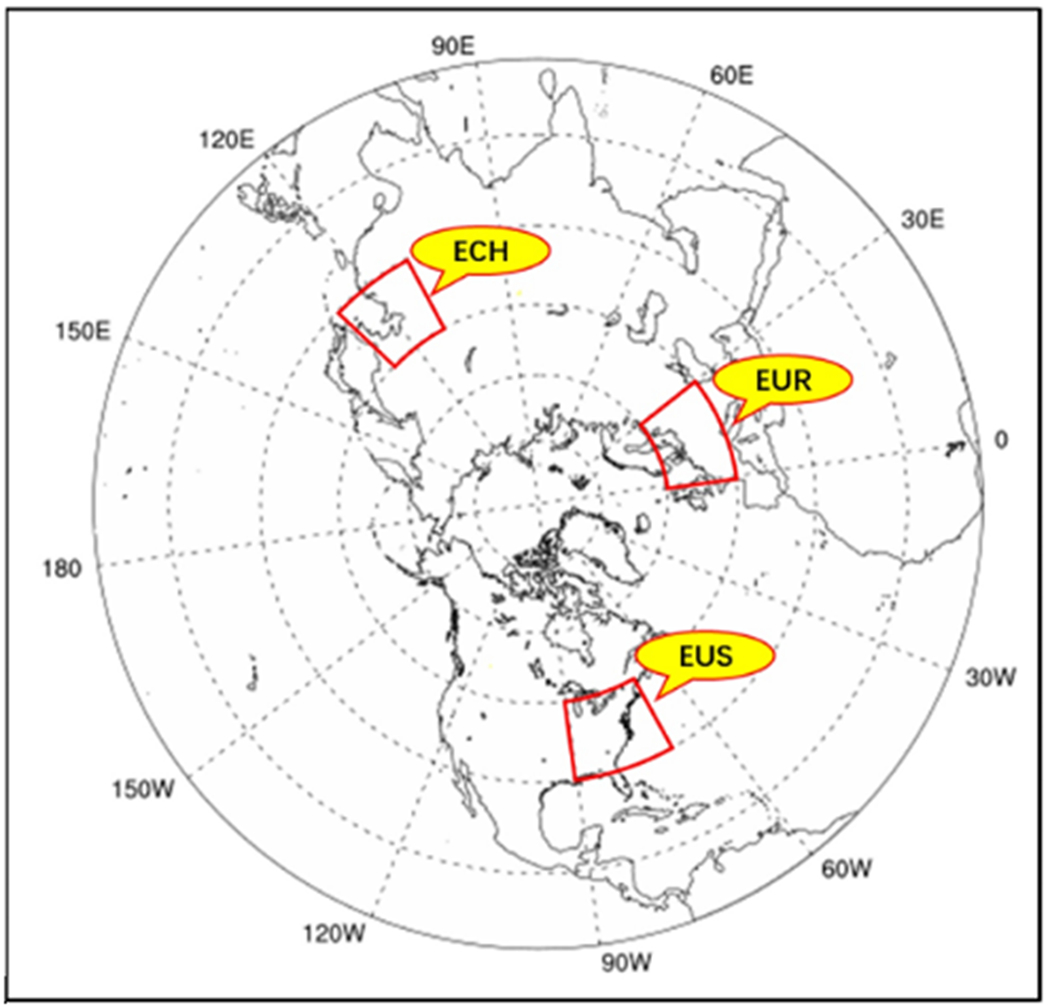
Simulation domain and targeted regions. ∗ Eastern China (ECH, 30°N-45°N, 110°E-130°E), Eastern US (EUS, 30°N-45°N, 90°W-70°W), and Europe (EUR, 45°N-60°N,0°E-30°E).
The model performance in the simulation of gaseous and particle concentrations was evaluated thorough comparison with several ground observation networks, including the air quality index provided by China National Environmental Monitoring Centre (CN-AQI, http://106.37.208.233:20035/), the European Monitoring and Evaluation Programme (EU-EMEP, http://www.emep.int), the European Air quality data Base (EU-AIRBASE, http://acm.eionet.europa.eu/databases/airbase/), the Air Quality System (US-AQS, http://www.epa.gov/ttn/airs/airsaqs/), and the Interagency Monitoring of Protected Visual Environments (US-IMPROVE, http://vista.cira.colostate.edu/improve/). Only data at sites that covered more than 75% of entire year are selected for the comparison. The monitors of CN-AQI, EU-AIRBASE and US-AQS are located predominantly in urban areas, while the monitors of EU-EMEP and US-IMPROVE are located in rural areas and represent the background conditions.
2.2. Sensitivity analysis
Simulations for the entire year of 2015 were conducted using the hemispheric WRF-CMAQ model, with a three-month spin-up period (October–December 2014). First, the base case (denoted as “Sim-base”) is conducted by using the PV-based STE-O3 parametrization in hemispheric CMAQ model. To quantify the influence of STE on surface PM2.5 concentrations, we conducted a controlled case (noted as “Sim-noSTE”) in which no STE-derived downward transport of O3 was simulated (i.e., the PV-based STE-O3 function was turned off). The O3 concentration through the column was initialized based on the default “clean” condition from 35 ppb (surface) to 70 ppb (top) at the beginning of the 3 month spin-up simulation. The Sim-base simulation was initialized with the O3-PV function with 3-months spin-up which is consistent with our previous study. And the difference between Sim-base and Sim-noSTE is noticeable after the 3 month spin-up (Fig. S4). Since other model options are the same as Sim-base, the difference between Sim-base and Sim-noSTE represents the impacts of STE on tropospheric O3 level and its subsequent influence on ground PM2.5 concentrations. The changes in simulated 24-h averaged O3, PM2.5 and its chemical components are calculated for evaluating the STE influence on both annual and seasonal averaged level.
In addition to examining these changes across the entire northern hemisphere, we selected three land regions (including adjacent ocean areas which might be impacted by transport from land) which are strongly impacted by anthropogenic emissions i.e., eastern China (ECH, 20N-40 N, 100E-125E), eastern US (EUS, 28N-50 N, 100W-70W), and Europe (EUR, 35N-65 N, 10W-30E), as shown in Fig. 1, for further analysis and comparison.
3. Results and discussion
3.1. Model evaluation
Table 1 summarizes the performance statistics of the comparison between observations and simulations (Sim-base) of gaseous and particle species. Generally, the model exhibits performance levels comparable to the previous studies (Xing et al., 2015a; Liu et al., 2020). For gaseous species, it captured the relatively higher concentrations of NO2 and SO2 in eastern China relative to the other two regions. The model also captured urban-rural concentration differences with higher concentrations of NO2 and SO2 in urban area (i.e., EU-AIRBASE) than rural area (i.e., EU-EMEP). But the discrepancy between urban and rural sites is significantly underestimated due to the coarse spatial resolution of the hemispheric model, resulting in low-biases in urban sites (CN-AQI, EU-AIRBASE, and US-AQS), but high-biases in rural sites (EU-EMEP). The model captured the average O3 concentrations, with the normalized mean biases (NMB) ranging from −9.1 to 39.8%. The overestimation of O3 in CN-AQI is mainly due to the coarse spatial resolution of the hemispheric model which fails to capture the strong VOC-limited condition in urban center with high NOx and low O3 levels (e.g., Ding et al., 2019a, Ding et al., 2019b). For particles, the model exhibits overestimation of PM2.5 components in EU-EMEP due to the high biases of the gaseous species. The simulated particulate nitrate (NO3−) and sulfate (SO42−) concentrations at locations of the US-IMPROVE are comparable to previous studies, with NMB of 43.5% and −22.2%, respectively. Due to the coarse spatial resolution, the model also underestimates the PM2.5 concentration by 29.4% in CN-AQI. In addition to the coarse resolution of the hemispheric model, the uncertainties associated with emission inventories, secondary particle formations (Zhang et al., 2019; Zhao et al., 2018), as well as no consideration of aerosol-radiative effects (Xing et al., 2015b; 2017b) might also contribute to such biases.
Table 1.
Statistic of model performance in simulating surface concentrations of gaseous and particle species.
| obs | sima | N | MB | NMB | Δsimb | ||||
|---|---|---|---|---|---|---|---|---|---|
| (μg/m3) | (μg/m3) | (pairs) | (μg/m3) | (%) | (μg/m3) | (%) | |||
| Gas | NO2 | CN-AQI | 31.8 | 9.3 | 17466 | −22.5 | −71.9 | −0.12 | −1.3% |
| EU-AIRBASE | 22.8 | 5.2 | 2976 | −17.6 | −77.2 | −0.20 | −3.8% | ||
| EU-EMEP | 1.6 | 3.7 | 502 | 2 | 118.5 | −0.21 | −5.8% | ||
| US-AQS | 8.5 | 3.2 | 407 | −5.3 | −62.7 | −0.03 | −1.0% | ||
| SO2 | CN-AQI | 26.1 | 10.5 | 17491 | −15.6 | −62.0 | −0.0039 | −0.04% | |
| EU-AIRBASE | 4.9 | 1.3 | 1664 | −3.6 | −73.7 | −0.0004 | −0.03% | ||
| EU-EMEP | 0.3 | 1 | 494 | 0.7 | 213.5 | 0.0005 | 0.05% | ||
| US-AQS | 1.2 | 0.3 | 430 | −0.9 | −71.9 | −6.00E-05 | −0.02% | ||
| O3 | CN-AQI | 55.9 | 74.2 | 17443 | 18.3 | 39.8 | 5.09 | 6.80% | |
| EU-AIRBASE | 54 | 63.8 | 2047 | 9.8 | 18.2 | 8.15 | 12.80% | ||
| EU-EMEP | 70.4 | 63.3 | 704 | −7.1 | −9.1 | 8.48 | 13.40% | ||
| Particles | PM2.5 | CN-AQI | 52.1 | 37.4 | 17420 | −14.8 | −29.4 | 0.24 | 0.70% |
| NO3− | EU-EMEP | 0.4 | 2.3 | 261 | 2 | 579.6 | 0.17 | 7.70% | |
| US-IMPROVE | 0.3 | 0.6 | 1800 | 0.2 | 43.5 | 0.03 | 5.60% | ||
| SO42− | EU-EMEP | 0.5 | 1 | 254 | 0.5 | 108.2 | −0.0030 | −0.3% | |
| US-IMPROVE | 0.8 | 0.6 | 1800 | −0.2 | −22.2 | −0.0011 | −0.2% | ||
| NH4+ | EU-EMEP | 0.5 | 1.1 | 266 | 0.5 | 92.4 | 0.04 | 3.80% | |
sim – the simulated concentrations in Sim-base, annual mean.
Δsim – represent the impacts of STE, derived from the differences in between Sim-Base and Sim-noSTE.
We also studied the differences between the two simulations in predicting the gaseous and particles at monitor sites (see Δsim as presented in Table 1). Generally, the model reflects the STE-derived downward transport of O3, as the surface O3 concentrations are enhanced by 5.1–8.5 μg m−3, about 6.8–13.4% of average surface O3 concentrations. The model also reflects the influence of the STE-enhanced O3 on atmospheric chemical formations, as we can see that all monitor locations show decreases of modeled NO2 and increases in modeled NO3−. The STE-enhanced O3 boosts the OH formation at daytime leading to an increased NO2-to-NO3 transition (Fig. S5). Meanwhile the formatting of N2O5 is also increased at night-time, result in a decrease of NO2 and enhanced HNO3 formation. The decrease in SO2 is also noticeable at urban sites (CN-AQI, EU-AIRBASE, and US-AQS) due to the increased oxidation of S(IV) to S(VI) driven by STE-enhanced O3. Opposite results are shown at rural sites (EU-EMEP and US-IMPROVE) which exhibit slightly increased SO2 and decreased SO42−. This may be due to the increased NO3− with limited availability of NH3 which causes a reduction in pH which then inhibits the pH-dependent oxidation of SO2 to SO42− by O3 (Seinfeld and Pandis, 2016). In general, the model is able to capture the pollution levels observed at all monitor sites. The reasonable performance of the base case simulation provides confidence in the use of the model and sensitivity run (Sim-noSTE) in assessing the effects of STE associated O3 on tropospheric PM2.5 levels.
3.2. Impacts of the STE on surface PM2.5 concentrations
Fig. 2 displays the spatial distribution of seasonal-average STE impacts on surface PM2.5 concentration across the northern hemisphere. In general, the surface PM2.5 concentration is enhanced by the STE enhanced tropospheric O3. The largest impact of STE is seen in winter when the atmospheric oxidation capacity is the lowest across the year and STE associated tropospheric O3 is relatively high (e.g., Xing et al., 2016; Mathur et al., 2017); thus the response of PM2.5 concentration to enhanced O3 exhibits greater sensitivity than other seasons. The STE-enhanced regional-average PM2.5 concentrations across East China, East US, and Europe are estimated to be 0.661, 0.251, and 0.594 μg/m3, respectively, which account for 1.3%, 3.5% and 5.5% of total PM2.5 concentrations. The STE impacts on PM2.5 are also noticeable over East China (0.318 μg/m3, about 0.7%) and Europe (0.192 μg/m3, about 2.2%) in spring when the STE-derived O3 downward transport is the greatest (Xing et al., 2016). The smallest impact is noted during summer when the STE-derived O3 downward transport becomes the smallest. Additionally, during summer enhanced thermal- and photo-chemistry result in higher levels of atmospheric oxidants and thus the atmospheric oxidation capacity reaches the highest in the northern hemisphere, resulting in a smaller sensitivity of PM2.5 to enhanced STE associated O3 than other seasons.
Fig. 2.

The spatial distribution of STE impacts on surface PM2.5 concentration across the northern hemisphere (Spring = MAM, Summer = JJA, Autumn = SON, and Winter = DJF, seasonal averages, unit: μg/m3).
We also investigated the diurnal variation of the STE impacts on surface PM2.5 and O3, as presented in Fig. 3. For better comparison, the baseline concentration is normalized to the average over the 24 h period. The hourly changes of PM2.5 and O3 due to the STE are averaged across a season for each hour of a day, and further normalized to the baseline concentration (relative change ratio from the baseline concentration). In general, the diurnal pattern of the STE impact is quite similar in all three regions and for both seasons. The normalized enhancement for O3 (i.e., relative change ratio) is fairly flat across all hours, indicating the same increasing ratio applied across the day and the enhancement is proportional to ambient O3 concentrations. Considering O3 baseline concentration is high in the afternoon (2-4 pm local time), the highest impact of STE on O3 is also high when the vertical mixing is the strongest across a day, leading to an additional enhancement of O3 peak concentrations. However, the normalized enhancement for PM2.5 is the largest in the morning (5–8am local time) and the lowest in the afternoon (3–7pm local time). Such diurnal variation is consistent with the baseline PM2.5 concentration, indicating that the increase ratio due to STE is even larger at the higher PM2.5 levels which resulting in a more significant enhancement for the peak PM2.5 (increased nonlinearly) and an even worse polluted situation.
Fig. 3.
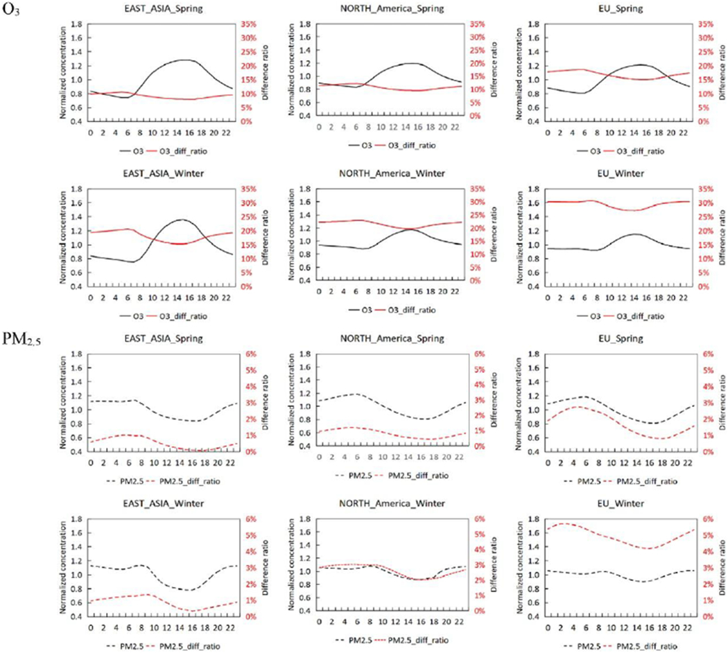
Diurnal variation of the STE impacts on surface O3 and PM2.5 in three selected regions (the blacklines present the normalized baseline concentrations at left-axis; the redlines present the increased ratio (_diff_ratio) by normalizing the STE impacts against with the baseline concentration at right-axis; solid lines represent the O3, and dashed lines represent the PM2.5).
3.3. Impacts of the STE on surface PM2.5 chemical components
We further investigate the STE impacts on each PM2.5 chemical components including SO42−, NO3−, ammonium (NH4+), and secondary organic aerosol (SOA), as shown in Fig. 4. We selected two seasons (i.e., spring and winter) with high STE-impacts for analysis. Compared to spring, larger STE impacts are found in winter for all chemical components. Compared to other components, NO3− is more sensitive to the STE-enhanced O3 in all regions, which accounts for 54-76% of the total STE-enhanced PM2.5. NH4+ and SOA are also influenced by the STE-enhanced O3, which accounts for 11-18% and 7-32% of the total STE-enhanced PM2.5. An interesting finding is that regional averages of SO42− decrease slightly across the northern hemisphere except in ECH wintertime when pollution is high. As we discussed previously in section 3.1, the decrease of SO42− might be associated with the reduced pH resulting from the increased NO3−. At the regional level, NH3 is limited and the enhanced NO3− will decrease the pH and inhibit the formation of SO42− through oxidation by O3. The opposite impacts on SO42− in ECH during spring and winter might be associated with the more abundant NH3 level in ECH compared to other regions (Wang et al., 2011). Because of the abundant NH3, the pH reduced much less due to the increase of NO3−, resulting in an facilitated oxidation of SO2 to SO42− by the STE-enhanced O3.
Fig. 4.

The STE impacts on surface concentrations of PM2.5 chemical components (a) and the share of PM2.5 chemical components in the STE impacts on total PM2.5 (b).
The three regions present similar shares of PM2.5 chemical components in the STE impacts on total PM2.5, except larger SOA is seen in East China during winter when heavy pollution frequently occurs compared to other regions and spring. The increased SOA enhancement in East China might be associated with the increasing sensitivity of SOA to O3 along with the increases of PM2.5 concentrations under which the more semi-volatile precursors can partition to the higher existing aerosols, as illustrated in Fig. 5 and further explored below.
Fig. 5.

The STE impacts on surface concentrations of PM2.5 and chemical components under different pollution levels in East China (the PM2.5 concentrations are 0–35, 35-115, 115-150, 150-250, 250-350, >350 μg/m3, respectively, at 5 pollution levels).
Compared to East US and Europe, East China exhibits the highest STE-enhanced PM2.5 and its components (Fig. 2, Fig. 4). That might be due to its high baseline concentrations. To demonstrate that, we further investigate the change of the STE impacts under different PM2.5 pollution levels in East China. Five pollution levels are defined based on the PM2.5 concentration ranges of 0–35, 35-115, 115-150, 150-250, 250-350, >350 μg/m3, respectively. In constructing Fig. 5 we further examined modeled daily mean PM2.5 concentrations and STE-induced changes (defined as the difference: Sim-base – Sim-noSTE) by averaging these daily values according to five PM2.5 concentration bins for these five pollution level. As shown in Fig. 5a, clear positive correlation between the STE-enhanced PM2.5 and the pollution levels are noted in all four seasons, indicting the stronger impacts of STE on PM2.5 under heavier polluted conditions. Additionally, the diurnal variations of STE impacts are significantly different at pollution Level 1 and 5 for both PM2.5 and O3 (see Fig. 5b). For STE-enhanced O3, the diurnal variations at Level 5 are much stronger than that at Level 1, indicating that the STE-enhanced O3 can play an important role in the chemical reactions during polluted period. The diurnal variations of PM2.5 present a peak in the morning (around 10 am), indicating the accumulation of pollutants through the night, and then reducing due to ventilation as the PBL grows. In East China wintertime, the impacts of STE are seen to be increasing along with the pollution levels for all PM2.5 chemical components (Fig. 5c). Meanwhile, the share of the STE-enhanced PM2.5 components varies quite differently for each components. As presented in Fig. 5d, the share of the STE-enhanced SOA increases with increasing pollution levels, while the share of the secondary inorganic aerosols (SNA, i.e., sum of SO42−, NO3− and NH4+) decreases. A possible reason is that the more semi-volatile precursors can partition to the higher existing aerosols, suggesting that the STE enhancement on SOA becomes more important under heavy polluted period. The share of SOA in total PM2.5 slightly increases along with the pollution level, which might also contribute to such increase of STE-enhanced SOA under the heavy polluted period (Fig. 5e–f). The wintertime SOA in East China mainly from the oxidation of anthropogenic VOC emissions, since the biogenic VOC emissions are at the lowest in winter. That implies the potential extra benefits of emission controls in reducing SOA concentrations from the mitigation of the STE enhancement effects.
4. Summary and conclusion
This study simulated the downward transport of O3 from the stratosphere using the hemispheric WRF-CMAQ model, evaluated the impacts of STE enhanced tropospheric O3 on surface PM2.5 concentrations, and suggested non-trivial enhancement of PM2.5 concentration due to the downward transport of O3 stemming from the STE. The results can be summarized as follows.
First, the largest STE-enhanced PM2.5 concentrations are mostly found in polluted regions including East China, East US, and Europe, and particularly in winter and spring. In winter, the STE-enhanced PM2.5 concentrations in East China, East US, and Europe are estimated to be 0.661, 0.251, and 0.594 μg/m3, respectively, on a seasonal average basis which accounts for 1.3%, 3.5% and 5.5% of total PM2.5 concentrations.
Second, different from the STE-enhancement O3 which exhibits the same increasing ratio across the day, the normalized STE-enhancement for PM2.5 is following a similar diurnal variation of baseline PM2.5 concentration, indicating that the increase ratio is even larger when PM2.5 concentration is already high (nonlinear enhancement). The results indicates that the STE enhances peak PM2.5 concentration thereby further exacerbating high pollution levels.
Third, the STE-enhanced PM2.5 is exclusively contributed by the increase of secondary aerosols which in turn are influenced by the atmospheric oxidation capacity. The STE-enhanced O3 has no impacts on primary aerosols (e.g., BC, Fig. S6). Among all PM2.5 components, NO3− is the most sensitive to the STE-enhanced O3 in all regions, which accounts for 70-75% of the total STE-enhanced PM2.5. However, the share of the STE-enhanced SOA increases with increasing pollution levels, further highlighting the importance of STE enhancement on SOA during heavy polluted period.
Uncertainties with the estimation of STE-O3 still exist. For example, the STE-O3 might be estimated due to the relatively short spin up time, although the difference between Sim-base and Sim-noSTE is noticeable after the 3 month spin-up (Fig. S4). Further analysis with longer spin-up period is suggested.
In summary, the downward transport of O3 stemming from STE can not only lead to an increase of surface O3 as most previous studies reported, but also result in an previously unquantified enhancement of ground-level PM2.5 concentration. Such impacts are estimated to be non-trivial in magnitude and could potentially be even higher during episodic intrusion events and in the future if frequency of STE events change due to climate change.
Supplementary Material
Acknowledgements
This work was supported in part by National Key R & D program of China (2017YFC0210006 & 2016YFC0208903), and National Natural Science Foundation of China (41907190). This work was completed on the “Explorer 100” cluster system of Tsinghua National Laboratory for Information Science and Technology. We thank Dr. Christian Hogrefe and Dr. Golam Sarwar for their help with the EPA internal review. The views expressed in this manuscript are those of the authors alone and do not necessarily reflect the views and policies of the U.S. Environmental Protection Agency.
Footnotes
Declaration of competing interest
The authors declare that they have no known competing financial interests or personal relationships that could have appeared to influence the work reported in this paper.
Appendix A. Supplementary data
References
- Albrecht B, 1989. A.: aerosols, cloud microphysics, and fractional cloudiness. Science 245, 1227e1230. [DOI] [PubMed] [Google Scholar]
- Ancellet G, Beekmann M, Papayannis A, 1994. Impact of a cutoff low development on downward transport of ozone in the troposphere. J. Geophys. Res.: Atmosphere 99 (D2), 3451e3468. [Google Scholar]
- Appel KW, Napelenok S, Hogrefe C, Pouliot G, Foley KM, Roselle SJ, et al. , 2018. Overview and evaluation of the community multiscale air quality (cmaq) modeling system version 5.2. Air Pollut. Model. Appl. Xxv 69e73. [DOI] [PMC free article] [PubMed] [Google Scholar]
- Bamber DJ, Healey PGW, Jones BMR, Penkett SA, Tuck AF, Vaughan G, 1984. Vertical profiles of tropospheric gases: chemical consequences of stratospheric intrusions. Atmos. Environ 18 (9), 1759e1766. [Google Scholar]
- Cohen AJ, Brauer M, Burnett R, Anderson HR, Frostad J, Estep K, Balakrishnan K, Brunekreef B, Dandona L, Dandona R, Feigin V, 2017. Estimates and 25-year trends of the global burden of disease attributable to ambient air pollution: an analysis of data from the Global Burden of Diseases Study 2015. Lancet 389 (10082), 1907e1918. [DOI] [PMC free article] [PubMed] [Google Scholar]
- Collins WJ, Derwent RG, Garnier B, Johnson CE, Sanderson MG, Stevenson DS, 2003. Effect of stratosphere troposphere exchange on the future tropospheric ozone trend. J. Geophys. Res 108 (D12), 8528 10.1029/2002JD002617. [DOI] [Google Scholar]
- Danielsen EF, 1968. Stratospheric-tropospheric exchange based on radioactivity, ozone and potential vorticity. J. Atmos. Sci 25, 502e518. [Google Scholar]
- Ding D, Xing J, Wang S, Chang X, Hao J, 2019a. Impacts of emissions and meteorological changes on China’s ozone pollution in the warm seasons of 2013 and 2017. Front. Environ. Sci. Eng 13 (5), 76. [Google Scholar]
- Ding D, Xing J, Wang S, Liu K, Hao J, 2019b. Estimated contributions of emissions controls, meteorological factors, population growth, and changes in baseline mortality to reductions in ambient PM 2.5 and PM 2.5-related mortality in China, 2013e2017. Environ. Health Perspect 127 (6), 67009. [DOI] [PMC free article] [PubMed] [Google Scholar]
- Forouzanfar MH, Collaborators GRF, 2015. Global, regional, and national comparative risk assessment of 79 behavioural, environmental and occupational, and metabolic risks or clusters of risks in 188 countries, 1990e2013: a systematic analysis for the Global Burden of Disease Study 2013. Lancet 386 (10010), 2287e2323. [DOI] [PMC free article] [PubMed] [Google Scholar]
- Guenther A, Hewitt CN, Erickson D, Fall R, Geron C, Graedel T, Harley P, Klinger L, Lerdau M, McKay WA, Pierce T, Scholes B, Steinbrecher R, Tallamraju R, Taylor J, Zimmerman P, 1995. A global model of natural volatile organic compound emissions. J. Geophys. Res 100, 8873e8892. [Google Scholar]
- Holton JR, Haynes PH, McIntyre ME, Douglass AR, Rood RB, Pfister L, 1995. Stratosphere-troposphere exchange. Rev. Geophys 33, 403e439 10.1029/95rg02097. [DOI] [Google Scholar]
- Lelieveld J, Dentener FJ, 2000. What controls tropospheric ozone? J. Geophys. Res 105, 3531e3551. [Google Scholar]
- Liu S, Xing J, Wang S, Ding D, Chen L, Hao J, 2020. Revealing the impacts of transboundary pollution on PM2. 5-related deaths in China. Environ. Int 134, 105323. [DOI] [PubMed] [Google Scholar]
- Mathur R, Xing J, Gilliam R, Sarwar G, Hogrefe C, Pleim J, Young J, 2017. Extending the Community Multiscale Air Quality (CMAQ) modeling system to hemispheric scales: overview of process considerations and initial applications. Atmos. Chem. Phys 17, 12449. [DOI] [PMC free article] [PubMed] [Google Scholar]
- McCaffery SJ, McKeen SA, Hsie E-Y, Parrish DD, Cooper OR, Holloway JS, Hübler G, Fehsenfeld FC, Trainer M, 2004. A case study of stratospheretroposphere exchange during the 1996 North Atlantic Regional Experiment. J. Geophys. Res 109 10.1029/2003JD004007. D14103 [DOI] [Google Scholar]
- McCormick RA, Ludwig JH, 1967. Climate modification by atmospheric aerosols. Science 156 (3780), 1358e1359. [DOI] [PubMed] [Google Scholar]
- Neu JL, Flury T, Manney GL, Santee ML, Livesey NJ, Worden J, 2014. Tropospheric ozone variations governed by changes in stratospheric circulation. Nat. Geosci 7 (5), 340e344. [Google Scholar]
- Price C, Penner J, Prather M, 1997. NOx from lightning 1: global distribution based on lightning physics. J. Geophys. Res 102 (D5), 5929e5941. [Google Scholar]
- Roelofs GJ, Lelieveld J, 1997. Model study of the influence of cross-tropopause O3 transports on tropospheric O3 levels. Tellus B 49, 38e55. [Google Scholar]
- Sarwar G, Luecken D, Yarwood G, Whitten GZ, Carter WPL, 2008. Impact of an updated carbon bond mechanism on predictions from the cmaq modeling system: preliminary assessment. J. Appl. Meteorol. Climatol 47, 3e14. [Google Scholar]
- Seinfeld JH, Pandis SN, 2016. Atmospheric Chemistry and Physics: from Air Pollution to Climate Change. John Wiley & Sons. [Google Scholar]
- Skamarock WC, Klemp JB, Dudhia J, Gill DO, Barker DM, G Duda M, Huang X-Y, Wang W, Powers JG, 2008. A description of the advanced Research WRF version 3. NCAR Tech. Note NCAR/TN-475þSTR 113 10.5065/D68S4MVH. [DOI] [Google Scholar]
- Stohl A, Spichtinger-Rakowsky N, Bonasoni P, Feldmann H, Memmesheimer M, Schell HE, Trickl T, Hübener S, Ringer W, Mandl M, 2000. The influence of stratospheric intrusions on alpine ozone concentrations. Atmos. Environ 34, 1323e1354. [Google Scholar]
- Wang S, Xing J, Jang C, Zhu Y, Fu JS, Hao J, 2011. Impact assessment of ammonia emissions on inorganic aerosols in East China using response surface modeling technique. Environ. Sci. Technol 45 (21), 9293e9300. [DOI] [PubMed] [Google Scholar]
- Xing J, Mathur R, Pleim J, Hogrefe C, Gan CM, Wong DC, Wei C, 2015b. Can a coupled meteorology-chemistry model reproduce the historical trend in aerosol direct radiative effects over the Northern Hemisphere? Atmos. Chem. Phys 15 (17). [Google Scholar]
- Xing J, Mathur R, Pleim J, Hogrefe C, Wang J, Gan CM, McKeen S, 2016. Representing the effects of stratosphereetroposphere exchange on 3-D O3 distributions in chemistry transport models using a potential vorticity-based parameterization. Atmos. Chem. Phys 16 (17), 10865. [Google Scholar]
- Xing J, Wang J, Mathur R, Wang S, Sarwar G, Pleim J, Hao J, 2017b. Impacts of aerosol direct effects on tropospheric ozone through changes in atmospheric dynamics and photolysis rates. Atmos. Chem. Phys 17 (16), 9869. [DOI] [PMC free article] [PubMed] [Google Scholar]
- Xing J, Wang S, Zhao B, Wu W, Ding D, Jang C, Zhu Y, Chang X, Wang J, Zhang F, Hao J, 2017a. Quantifying nonlinear multiregional contributions to ozone and fine particles using an updated response surface modeling technique. Environ. Sci. Technol 51 (20), 11788e11798. [DOI] [PubMed] [Google Scholar]
- Xing J, Mathur R, Pleim J, Hogrefe C, Gan C-M, Wong DC, Wei C, Gilliam R, Pouliot G, 2015a. Observations and modeling of air quality trends over 1990e2010 across the Northern Hemisphere: China, the United States and Europe. Atmos. Chem. Phys 15, 2723e2747 10.5194/acp-15-2723-2015. [DOI] [Google Scholar]
- Zanis P, Hadjinicolaou P, Pozzer A, Tyrlis E, Dafka S, Mihalopoulos N, Lelieveld J, 2014. Summertime free-tropospheric ozone pool over the eastern Mediterranean/Middle East. Atmos. Chem. Phys 14, 115e132 10.5194/acp-14-115-2014. [DOI] [Google Scholar]
- Zhang S, Xing J, Sarwar G, Ge Y, He H, Duan F, Chu B, 2019. Parameterization of heterogeneous reaction of SO2 to sulfate on dust with coexistence of NH3 and NO2 under different humidity conditions. Atmos. Environ 208, 133e140. [DOI] [PMC free article] [PubMed] [Google Scholar]
- Zhao B, Zheng H, Wang S, Smith KR, Lu X, Aunan K, Fu X, 2018. Change in household fuels dominates the decrease in PM2. 5 exposure and premature mortality in China in 2005e2015. Proc. Natl. Acad. Sci. Unit. States Am 115 (49), 12401e12406. [DOI] [PMC free article] [PubMed] [Google Scholar]
Associated Data
This section collects any data citations, data availability statements, or supplementary materials included in this article.