Abstract
Objectives:
High throughput pre-treatment imaging features may predict radiation treatment outcome and guide individualized treatment in radiotherapy (RT). Given relatively small patient sample (as compared with high dimensional imaging features), identifying potential prognostic imaging biomarkers is typically challenging. We aimed to develop robust machine learning methods for patient survival prediction using pre-treatment quantitative CT image features for a subgroup of head-and-neck cancer patients.
Methods:
Three neural network models, including back propagation (BP), Genetic Algorithm-Back Propagation (GA-BP), and Probabilistic Genetic Algorithm-Back Propagation (PGA-BP) neural networks were trained to simulate association between patient survival and radiomics data in radiotherapy. To evaluate the models, a subgroup of 59 head-and-neck patients with primary cancers in oral tongue area were utilized. Quantitative image features were extracted from planning CT images, a novel t-Distributed Stochastic Neighbor Embedding (t-SNE) method was used to remove irrelevant and redundant image features before fed into the network models. 80% patients were used to train the models, and remaining 20% were used for evaluation.
Results:
Of the three supervised machine-learning methods studied, PGA-BP yielded the best predictive performance. The reported actual patient survival interval of 30.5 ± 21.3 months, the predicted survival times were 47.3 ± 38.8, 38.5 ± 13.5 and 29.9 ± 15.3 months using the traditional PCA. Combining with the novel t-SNE dimensionality reduction algorithm, the predicted survival intervals are 35.8 ± 15.2, 32.3 ± 13.1 and 31.6 ± 15.8 months for the BP, GA-BP and PGA-BP neural network models, respectively.
Conclusion:
The work demonstrated that the proposed probabilistic genetic algorithm optimized neural network models, integrating with the t-SNE dimensionality reduction algorithm, achieved accurate prediction of patient survival.
Advances in knowledge:
The proposed PGA-BP neural network, integrating with an advanced dimensionality reduction algorithm (t-SNE), improved patient survival prediction accuracy using pre-treatment quantitative CT image features of head-and-neck cancer patients.
Introduction
Head-and-neck cancer (HNC) is the sixth leading cancer by incidence worldwide. The annual incidence of HNC is more than 550,000 cases with approximate 300,000 deaths per year1 . Oral tongue cancer is a subsite and one of the most common HNC, the overall 5 year survival rates have remained low at approximately 50%, considerably lower than other cancer such as colorectal, cervix and breast cancers.2 Common treatments of oral cancer mainly include radiotherapy, chemotherapy, and surgery. These treatments are often combined in clinic to minimize morbidity and mortality and improve the patients' quality of life.3 The accurate prediction of prognosis and survival may be the first step for the selection of individualized therapy for the cancer patients. For example, if a patient who might have a short survival period, he or she probably will not be able to benefit from the surgical treatment and is suitable for palliative irradiation or supportive care. The patient can have surgery if he has a good prognosis and is in general condition, and some patients may even receive metastatic tumor excision to better control local diseases.4
Traditional survival predictions have focused on the use of genomic and proteomic techniques, which generally need a biopsy invasive surgery to remove a small portion of tumor tissue for analysis. However, a single biopsy can't fully assess the tumor's heterogeneity in space and time, and multiple consecutive biopsies are generally not practical.5 Medical images, providing non-invasive patient specific information of the entire tumor with relative no additional or low cost, are often used to monitor the tumor occurrence, development, and response to treatment, etc.6 A typical radiation treatment usually generated a large pool of patient specific data involving multimodality images.
Radiomics is an emerging field that extracts quantitative image features from medical images and analyses them to find imaging markers of disease, so as to achieve accurate prediction, diagnosis, and prognosis of diseases.7 Radiomics features (including intensity, shape, texture, etc) offer information on cancer phenotype as well as the tumor microenvironment that is distinct and complementary to the patient data.8 The quantitative imaging features have great potential in guiding treatment, which can provide a new method for predicting the survival of cancer. Many literatures5–9 demonstrated that the significant correlations between quantitative image features with patient RT outcome. In 2014, a study published by Aerts et al,5 who extracted 440 quantitative tumor image features, including grayscale, texture, shape, and wavelet from CT data of 1019 lung or head and neck neoplasm patients. These imaging features reflecting heterogeneity of tumor are associated with specific pathological type, T stage, and pattern of gene expression. These features have also shown good prognostic values in multiple atypical lung or head and neck neoplasm databases. Coroller et al8 extracted 635 features from CT images of lung adenocarcinoma patients to predict distant metastasis and survival with imaging method, among which 35 features were related to distant metastasis and 12 features were related to survival. Leijenaar et al10 reported the good prognostic value using pre-treatment CT imaging features from a group of 542 patients with oropharyngeal squamous cell carcinoma.
One of current great challenge of Radomics analysis is the lack of effective methodologies to characterize substantially large number of quantitative features extracted from images in order to study their association with clinical outcome. As a heuristic optimization algorithm, genetic algorithm (GA) has achieved good results in many fields. In recent years, some improved genetic algorithms have been studied in multicast routing,11 model prediction,12 optimal design13 and other fields. 14–16 Furthermore, many studies have proved that GA and its improved algorithm can optimize some kinds of neural networks, and have made research achievements in water level prediction,17 model fitting,18 mining method optimization,19 stock market index prediction20 and so on.21–24
In this paper, we developed robust neural network models to access clinical treatment outcome in radiation therapy (RT). To predict the survival of patients, the probabilistic adaptive genetic algorithm (PGA) combined with back propagation neural network is proposed. Due to the nature of high-dimensional non-linear of the Radiomics features, this work introduced a novel t-Distributed Stochastic Neighbor Embedding (t-SNE) algorithm for non-linear dimensionality reduction, and then utilized the PGA-BP neural network for survival prediction. For a group of oral HNC patients, the PGA-BP neural network model yielded highest prediction accuracy compared with the BP neural network and traditional GA-BP neural network models. The accurate prediction of survival may further facilitate clinical decision-making to optimize the treatment outcome.
Methods
Patient
A subgroup of 59 H&N squamous cell carcinoma patients, with primary tumor location at base-of-tongue, tonsil, or oral tongue, treated at a single institution was included in the study. The average age of this patient group is 60 ± 23(years). All patients underwent their initial external beam radiation therapy with prescription dose of 69.3 Gy (in 33 fractions) to gross tumor volume (GTV). The patients with available survival information in our database were included. The study excludes those recurrence patients who received previous RT and surgery.
Image features
All patients underwent a pre-treatment CT scan for treatment planning purpose at a same CT scanner - Siemens Sensation Open CT (Siemens Healthineers AG, Munich, Germany) prior to their radiation therapy. The standard H&N clinical CT acquisition and reconstruction protocol were used for all patients. The GTV was delineated by the attending from the planning CT. A total of 1386 quantitative image features, including Shape, Intensity Direct, Intensity Histogram, Gray Level Co-occurence Matrix, Neighbor Intensity Difference were extracted from the GTV for each patient using an open infrastructure software platform IBEX.25 These features are considered as potential predictors to feed as inputs for the prediction models.
Feature dimensionality reduction
The extracted high-dimensional imaging features may contain a large amount of irrelevant and redundant information. Feature reduction algorithm is expected to reduce the number of unimportant imaging features while retaining the main features for survival predictions. We utilized the commonly used principal component analysis (PCA), and an emerging machine learning algorithm called t-SNE to remove redundant and irrelevant (or minor) features to hopefully improve prediction accuracy.
Principal component analysis (PCA)
The unprocessed high-dimensional imaging data may reduce the computational efficiency, but also have a negative impact on subsequent prediction accuracy. Dimensionality reduction algorithms, such as PCA, are generally needed to remove irrelevant features before fed into neural network models. The PCA converts possibly correlated high-dimensional observations into a set of linearly uncorrelated variables called principle components via co-ordinate transformation, a covariance matrix is used to calculate the transformation.26 The PCA method is proven to retain the characteristics of the original data to the utmost extent.27–30
Givena matrix X composed of n rows (number of patients) and m columns (features). First, we normalize the data by subtracting the respective means of the row for each value of each row. Second, we calculated covariance matrix and the eigenvalues with corresponding eigenvectors. Finally, we chose the eigenvectors arranged into a matrix according to the corresponding eigenvalue size and formed a matrix P. Matrix P is the data after dimension reduction to K dimension. The k value was determined to balance the minimized number of features while retaining as much information as possible (at least 90% information was retained).
T-distributed stochastic neighbor embedding (t-SNE) algorithm
In addition, an emerging non-linear dimension reduction algorithm, t-SNE algorithm,31 is employed and compared with the PCA in this work. The t-SNE is a non-linear dimensionality reduction algorithm using for manifold learning.32 It maps high-dimensional data to low-dimensional space (using t-distribution) for human observation and analysis. It has demonstrated that the t-SNE has the best dimensionality reduction effect in the same algorithm and is widely applied in medical analysis, biological exploration, computer image research33 The basic idea of t-SNE algorithm is to represent the similarity of data points with joint probability between high-dimensional data points. We can simulate data points of the corresponding low-dimensional space, and obtain the best low-dimensional simulation data points by minimizing the KL divergence.34–36
The condition probability (the probability of event A condition has occurred in a further event B) and between the two data points among imaging feature matrix can be formulated as:
| (1) |
| (2) |
Where i and j are number of patients. Among which, is the vector variance of Gaussian function centered on data point in the matrix, is Patients characteristic value.
When t-distribution is used in a low-dimensional space and the degree of freedom is 1, the joint probability (the probability of two events occurring together) between the two data points simulated in the low-dimensional space is expressed by:
| (3) |
The correct metric KL relates of the two points in the high dimensional matrix and of the two data points simulated in the low-dimensional space:
| (4) |
To ensure the correctness of the simulated data, it is necessary to minimize the KL divergence. The result of optimized KL divergence by the gradient descent method is:
| (5) |
Where are features after dimensional reduction.
Neural network models
Given the large number of potential predictors extracted from medical images, it is extremely challenge to identify a set of optimal features for meaningful outcome response prediction via radiational statistical methods. Neural network models are used for modelling complex relationships between inputs (image features) and outputs (clinical end points such as patient survival) in this work.
Back propagation (BP) neural network
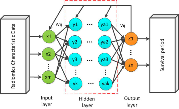
A schematic diagram of the back propagation (BP) network37 is shown in Figure 1. While forward propagation is training input into the network to obtain impulse responses, BP is impulse responses corresponding to the same target output training input differencing to obtain a response error of hidden layer and output layer. The error after output is used to estimate the error of the direct pre-layer, and uses this error to estimate the error of the previous layer. In the BP neural network, a single sample has m inputs,n outputs and k hidden layers between the input layer and the output layer. The simple three-layer network can include the input layer (I), the hidden layer (H), and the output layer (O).
Figure 1.
A schematic diagram of a m × k× n three-layer BP neural network. BP, back propagation.
Radiomics characteristic data as input data into training, the number of input parameters and input layer neurons are consistent. Each input neuron accepts one parameter, and the multilayered neuron can have multiple intermediate layers. The initial weights are connected between the neurons, and finally the output layer is established. Output predicted values of patient survival.
A basic 3-layer BP neural network structure was used with following pre-defined parameters. The number of input layer nodes, the hidden layer nodes and output nodes are 159, 25 and 1, respectively. The initial weight of network is set randomly. The transfer function of the implicit layer is S-type function,38 and the output layer's function is linear transfer function ,39 the training function is 40 which is a multilayer perceptron with gradient descent (GD) and BP with adaptive learning rate (LR), the performance function is the mean squared error ).41 We chose the learning rate of 0.01 and the target error of 0.00004 based on our experience.
Genetic algorithm-back propagation (GA-BP) network model
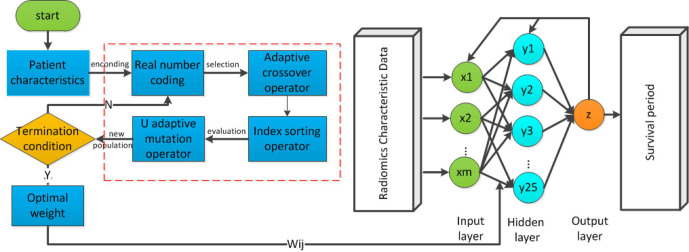
To overcome the issues of local minimum in the BP network, the GA was integrated in this paper.27 The GA is a parallel random search optimization method which formed by simulating the genetic mechanism of nature and biological. GAs is to simulate natural selection and genetic mechanism of Darwinian evolution of computational models of biological evolution. The process is a way to search for the optimal solution by simulating natural evolution. Although the poor individuals were eliminated, the new population inherited the information of the last generation, which is superior to the previous generation. The evolution cycle kept on going repeatedly until the terminal conditions were met. The purpose of the integration of GA to BP neural network is to optimize the initial weights and thresholds of the BP neural network. The flowchart of GA-BP network is illustrated in Figure 2.
Figure 2.
The general structure of genetic algorithms.
The GA is a global optimization algorithm, however, the GA itself has problems such as low search efficiencyand easy precocity. Optimizing BP neural network with simple genetic algorithm may lead to the deviation of search direction and immature convergence.
Probabilistic genetic algorithm-back propagation (PGA-BP) neural network
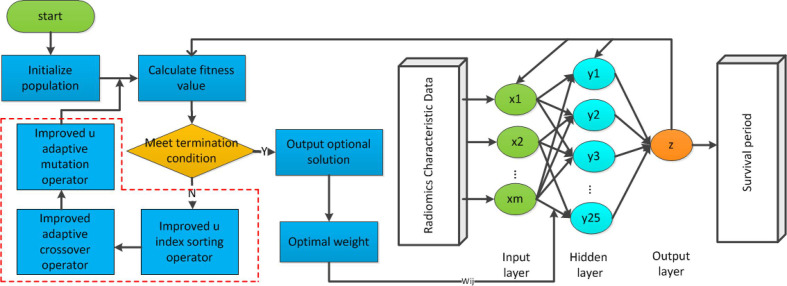
To improve the efficiency of optimization in GA-BP model, we proposed PGA-BP neural network in this work. The cross-over probability and the mutation probability are determined by the fitness. With the evolutionary operators, the weight of the BP neural network is optimized by genetic algorithm. In this model, the input is the training patients with radiomics characteristic. The number of input layer neurons is consistent with the patients’ features. Each neuron accepts one feature. The hidden layer has 25 points, and the initial weights are connected between the neurons. Finally, the output layer is built and has only one neuron. The final output is patient's survival prediction value. The PGA-BP training process optimized by GA based on probability adaptation is shown in Figure 3.
Figure 3.
The flowchart of PGA-BP neural network model. PGA-BP, probabilistic genetic algorithm-back propagation.
Encoding
A set of initial weights in the BP network constitutes an individual or a solution in the population. In this paper, real-encoding was adopted. The encoding length is:
| (6) |
where m is the node number in hidden layer; n is the node number in input layer; l is the node number in output layer.
Fitness function
Fitness is used to measure the quality of an individual. The formula is as follows:
| (7) |
Where is the coefficient; is the cases of training samples, is the number of output nodes; is the expected output value of the -th output neuron of the -th training sample; is the predicted output of the -th output neuron of the -th training sample value. The fitness function uses the reciprocal of the error. The larger the error is, the smaller the fitness is.
Index ordering & operator selecting
Individuals’ fitness in the group is sorted from the largest to the smallest. With the probability of selecting individual fitness decreases proportionally reduced.
| (8) |
| (9) |
| (10) |
Where is the probability of the individual's selection; N is the number of group; is the maximum fitness value, and is the average fitness value.
Adaptive crossover operator
The improved cross-over probability is as follows:
| (11) |
Where is the cross-over probability, is the initial cross-over probability, the value is taken as 0.8; is the larger fitness value of the two individuals to be cross-over, is the maximum fitness value, is the average fitness value; is coefficient between , the value is 0.4.
Suppose that individuals and perform cross-operations. For the bit , If the generated random number is less than the cross-over probability , the weight in and at this position will perform as following
| (12) |
Where is a random number among .
Mutation operator
For the mutation operator, the mutation probability is too small, which affects the optimization ability of genetic algorithm, the mutation probability is too large, and the excellent individual with large fitness may be destroyed23 The probability of individual genetic mutation should decrease as the number of evolution increases.24 Therefore, the mutation probability is improved in this paper for the above characteristics, and the probability formula of the mutation operator is:
| (13) |
Where is the mutation probability, is the initial mutation probability, the value is 0.4. is the individual fitness value to be mutated, is the maximum fitness value, is the average fitness value; is a coefficient, and the value is between , the value is 0.3; is a coefficient, and the value is between . The value is taken as 0.1; is the current number of iterations; =2, which is to prevent the probability from over decreasing when the number of iteration is 1.
The mutation operation selects the-th gene of the-th individual for mutation, and the mutation operation is as follows:
| (14) |
In the above formula, is the upper bound of gene ; is the lower bound of gene , , is a random number, is the current number of iterations, is the maximum number of evolution, is a random number between .
Model parameters
We used MATLAB R 2010b (The Math Works, Inc., Natick, MA) to achieve the construction, training and simulation of the prediction models. After the feature dimension reduction, 47 cases (80%) were used to construct the prediction models, and the remaining 12 cases (20%) were used for testing set.
The relevant parameters for GA-BP and PGA-BP used were: the population size is 10, the evolution frequency is 50, the initial cross-over probability is 0.8, the cross-over coefficient is 0.4, and the initial mutation probability is 0.4, the coefficient of variation is 0.3, the coefficient of variation is 0.1.
K-fold cross-validation
We utilized k-fold cross-validation to take as much effective information as possible from the limited data to minimize potential over fitting. Specifically, we randomly divided the patient sample into four independent cohorts, with three of them used for training, while the remaining one used for evaluation. The fourfold cross-validation reduces the variance by averaging the results of four different group trainings, the performance of the model is less sensitive to the partitioning of the data.
Results
Prediction of patient survival
After feature reduction, the remaining image features were fed into three neural network models for predictive modelling. Table 1 summarized the actual patient survival and the predicted results using BP, GA-BP and PGA-BP models when the PCA was utilized to perform feature reduction. For the evaluation cohort, the average of reported patient survival interval (and standard deviation, SD) is 30.5 ± 21.3 months, the predicted survival intervals (and SD) are 47.3 ± 38.8, 38.5 ± 13.5 and 29.9 ± 15.3 months for the BP, GA-BP and PGA-BP neural network models, respectively. The relative errors, defined as the ratio of the differences between the predicted survival and the actual survival time normalized by the actual survival time, were 2.65, 1.11 and 0.5 respectively for the three neural network models.
Table 1.
(a) Prediction results of three model after the PCA feature reduction.(b) Prediction results of three models after t-SNE feature reduction
| BP | GA-BP | PGA-BP | |||||
| Patient's No. | Survival period(month) | Prediction(month) | Relative error | Prediction(month) | Relative error | Prediction(month) | Relative error |
| 48 | 28.5 | 18.2 | 0.36 | 20.3 | 0.29 | 25.7 | 0.1 |
| 49 | 3.4 | 40.7 | 10.97 | 15.4 | 3.53 | 3.3 | 0.03 |
| 50 | 75.5 | 45.3 | 0.4 | 58.5 | 0.23 | 60.4 | 0.2 |
| 51 | 20 | 56.6 | 1.83 | 36.2 | 0.81 | 29.5 | 0.48 |
| 52 | 45.8 | 57.3 | 0.25 | 49.3 | 0.08 | 30.1 | 0.34 |
| 53 | 15.9 | 23 | 0.45 | 40.2 | 1.53 | 20 | 0.26 |
| 54 | 10.9 | 161.5 | 13.81 | 58.7 | 4.39 | 41.4 | 2.8 |
| 55 | 21.1 | 45.4 | 1.15 | 42.5 | 1.01 | 30.3 | 0.43 |
| 56 | 26.6 | 9.1 | 0.66 | 35.8 | 0.35 | 15.1 | 0.43 |
| 57 | 15.5 | 36 | 1.32 | 26.3 | 0.7 | 23.7 | 0.53 |
| 58 | 44.6 | 33.2 | 0.26 | 35.1 | 0.21 | 29.3 | 0.34 |
| 59 | 58.4 | 41.4 | 0.29 | 43.7 | 0.25 | 50.3 | 0.14 |
| Average | 30.5 | 47.3 | 2.65 | 38.5 | 1.11 | 29.93 | 0.51 |
| BP | GA-BP | PGA-BP | |||||
| Patient's no. | Survival period(month) | Prediction(month) | Relative error | Prediction(month) | Relative error | Prediction(month) | Relative error |
| 48 | 28.5 | 35.3 | 0.24 | 30.4 | 0.07 | 29.9 | 0.05 |
| 49 | 3.4 | 25.2 | 6.41 | 13.2 | 2.88 | 5.3 | 0.56 |
| 50 | 75.5 | 30.5 | 0.6 | 48.3 | 0.36 | 62.1 | 0.18 |
| 51 | 20 | 45.5 | 1.28 | 35.2 | 0.76 | 26.5 | 0.33 |
| 52 | 45.8 | 55.6 | 0.21 | 49.7 | 0.09 | 46.3 | 0.01 |
| 53 | 15.9 | 39.8 | 1.5 | 35.1 | 1.21 | 21.3 | 0.34 |
| 54 | 10.9 | 40.7 | 2.73 | 38.5 | 2.5 | 24.4 | 1.24 |
| 55 | 21.1 | 43 | 1.04 | 32.9 | 0.56 | 30.5 | 0.45 |
| 56 | 26.6 | 11.1 | 0.58 | 15.3 | 0.42 | 19.1 | 0.28 |
| 57 | 15.5 | 8.6 | 0.45 | 10.4 | 0.33 | 21.8 | 0.41 |
| 58 | 44.6 | 57.7 | 0.29 | 35.3 | 0.21 | 40.2 | 0.1 |
| 59 | 58.4 | 36.8 | 0.37 | 43.7 | 0.25 | 51.7 | 0.11 |
| Average | 30.5 | 35.8 | 1.31 | 32.3 | 0.81 | 31.6 | 0.34 |
BP, Back Propagation ; GA-BP, Genetic Algorithm-Back Propagation ; PGA-BP, Probabilistic Genetic Algorithm-Back Propagation ; t-SNE, t-Distributed Stochastic Neighbor Embedding.
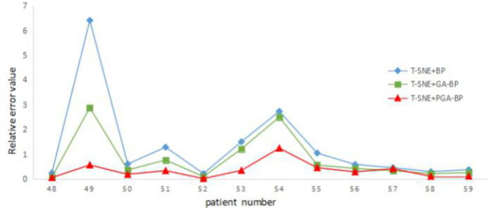
Table 1 (b) summarized the prediction results using BP, GA-BP and PGA-BP models using the t-SNE as feature reduction algorithm. The predicted survival intervals are 35.8 ± 15.2, 32.3 ± 13.1 and 31.6 ± 15.8 months for the BP, GA BP and PGA-BP neural network models, respectively. The relative errors are 1.31, 0.81 and 0.34 respectively.
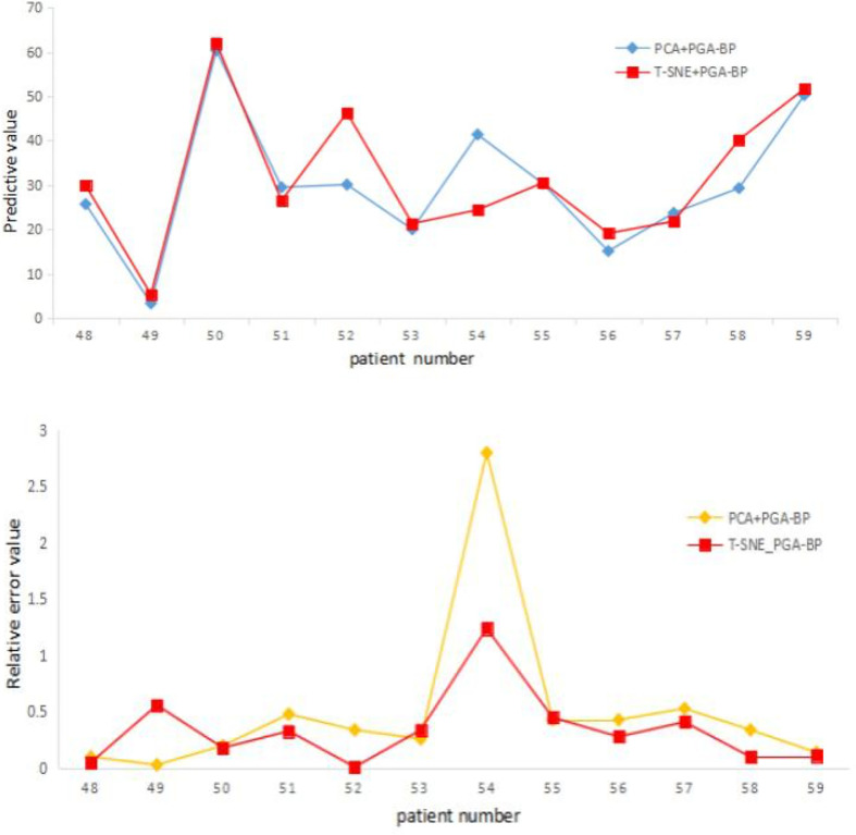
Figure 4 shows (a) predicted survival time and (b) relative errors given by the PGA-BP model when different feature reduction algorithms were used.
Figure 4.
(a) The survival period and (b) relative error distribution map of PCA + PGA BP and t-SNE + PGA BP. PCA, principal componene analysis; PGA-BP, Probabilistic Genetic Algorithm-Back Propagation; t-SNE, t-Distributed Stochastic Neighbor Embedding.
For the same prediction model, the relative error in survival period after t-SNE dimensional reduction are generally better than that of PCA, indicting the dimensional reduction capability of t-SNE is better than that of PCA. This is potential due to the complexity of non-linear high-dimensional nature in Radiomics feature data, the t-SNE algorithm can map non-linear high preserve good dimensional reduction capability for complex non-linear high-dimensional data, while the PCA is generally applicable to linear data.
Figure 5 illustrates the relative errors for different prediction models when the t-SNE was adopted for feature reduction. Among three neural network models, the PGA-BP model yielded smallest prediction errors.
Figure 5.
Relative error distribution map of t-SNE + three neural network models. PGA-BP, Probabilistic Genetic Algorithm-Back Propagation; t-SNE, t-Distributed Stochastic Neighbor Embedding.
Potential imaging predictors to patient survival
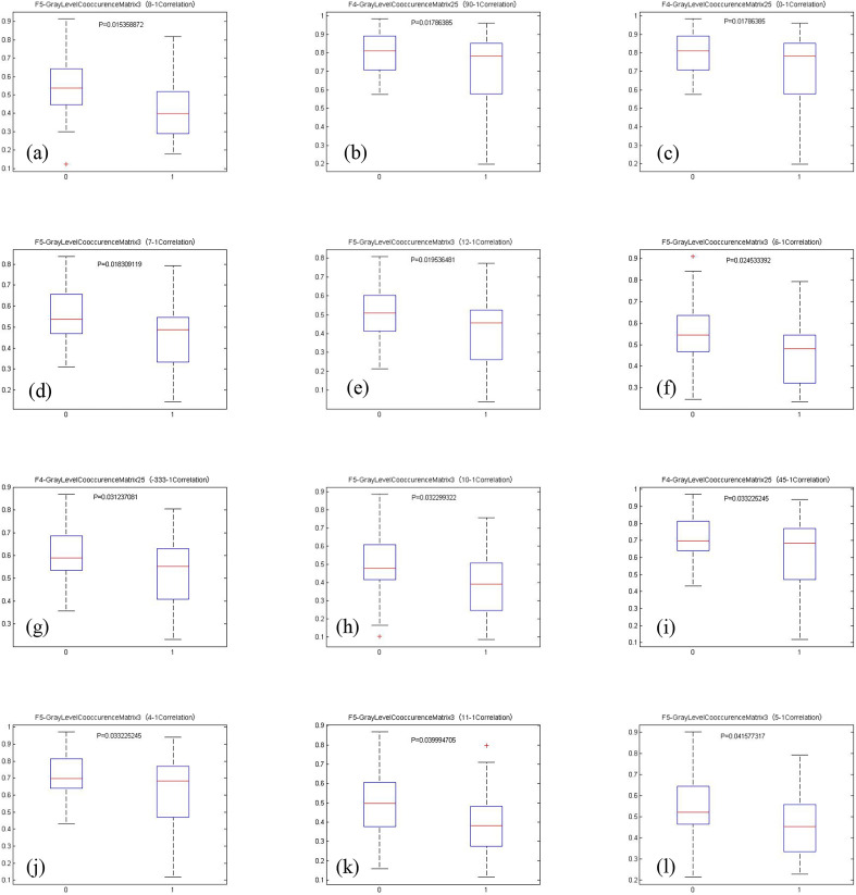
We divided the patients into two groups according to their survival time. For those patients with a survival time of 0–36 months, labeled as 0 (or short survival time group); for those patients with a survival time of more than 36 months, labeled as 1 (or long survival time group). t-Tests were performed to test the differences between these two groups with a cut-off value of p-value = 0.05.
(Figure 6) (a–i) Boxplots showing group differences of the identified imaging features using PGA-BP. 0 for short survival time group, 1 for long survival time group. A total of 12 features were selected and shown. The p-values < 0.05 are considered as statistically significant between group 0 and 1.
Figure 6.
(a–i) shows boxplots and p-values for the twelve important imaging features identified by the PGA-BP. The differences between long and short survival time patients are significant (the p-values are all less than 0.05) using the selected image features, suggesting the selected imaging features may largely affected patient survival time. The identified important features are all texture features related parameters characterized by GLCM features. GLCM, Gray Level Co-occurrence Matrix; PGA-BP, PGA-BP, Probabilistic Genetic Algorithm-Back Propagation.
Fourfold cross-validation results
The prediction results given by BP, GA-BP and PGA-BP models were tabulated in Table 2. The stability of BP network is poor. The average relative error of four groups of data is 1.60, and the standard deviation is 0.51. While the PGA-BP network is relatively stable. The average relative error of four groups of data is 0.36, and the standard deviation is only 0.04, which shows that the network has strong stability. PGA-BP network achieved better prediction.
Table 2.
The average prediction results by fourfold cross-validation
| Group | Average survival interval (months) | BP | GA-BP | PGA-BP | |||
| Average prediction (months) | Average relative error (months) | Average prediction (months) | Average relative error (months) | Average prediction (months) | Average relative error (months) | ||
| 1 | 34.90 ± 16.50 | 46.37 ± 18.58 | 2.46 ± 1.13 | 37.48 ± 15.35 | 1.22 ± 0.77 | 35.93 ± 13.55 | 0.41 ± 0.28 |
| 2 | 33.42 ± 20.25 | 39.65 ± 14.94 | 1.36 ± 1.27 | 36.27 ± 12.88 | 0.86 ± 0.73 | 34.65 ± 11.49 | 0.38 ± 0.26 |
| 3 | 18.98 ± 10.34 | 22.14 ± 9.68 | 1.27 ± 1.15 | 21.66 ± 8.65 | 0.78 ± 0.63 | 20.46 ± 7.62 | 0.31 ± 0.23 |
| 4 | 30.54 ± 20.43 | 35.82 ± 14.57 | 1.31 ± 1.69 | 32.33 ± 12.55 | 0.81 ± 0.89 | 31.59 ± 15.15 | 0.34 ± 0.32 |
| Avg. | 29.45 ± 16.88 | 35.99 ± 14.44 | 1.60 ± 1.31 | 31.94 ± 12.36 | 0.92 ± 0.75 | 30.66 ± 11.95 | 0.36 ± 0.27 |
PGA-BP, Probabilistic Genetic Algorithm-Back Propagation.
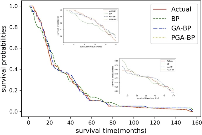
Figure 7 shows the predicted survival curves of different models compared to the actual survival curve. The BP, GA-BP, PGA-BP models yielded decent survival predictions from 0 to 160 months of follow-up period in general, the survival curve given by the PGA-BP appeared to be the closest match compared to the other two models, especially in 0–20 months.
Figure 7.
Survival prediction given by the BP, GA-BP, PGA-BP neutral network models. PGA-BP, Probabilistic Genetic Algorithm-Back Propagation
Discussion
We demonstrated the use of robust machine learning methods for treatment outcome predictions in radiation therapy. One of the greatest challenges of clinical outcome assessment is the patient heterogeneity. Large amount of patient specific information, including patient characteristics, clinical information, patient specific pathology, radiomics features, dosimetric information, radiomics and radiogenomics, etc is generally used to characterize patient heterogeneity, and believed to be associated with patient treatment outcome. Among all, to avoid overfitting, it is crucial to identify a subset of patient related information that most related to treatment outcome. One strength of this work is the adoption of the novel powerful t-SNE method to remove non-important or redundant information from high-dimensional quantitative tumor features (1386), which resulted in more accurate prediction results. To our best knowledge, this is the first time the t-SNE method was introduced for patient survival analysis in RT. The second strength of the work is the use of advanced neural network models for survival prediction. As a result, we demonstrate that the integrating the feature reduction and neural networks for accurate survival prediction, compared to the traditional BP neural network based on radiologic data of tongue carcinoma. The third strength of the study is the selected subsite of H&N patients with similar primary disease at oral tongue were included. All data were from a same institution and from the same scanner, so the CT acquisition and image reconstruction were considered to be consistent.
We utilized and compared three neural network models to predict patient survival. The simple BP neural network model yielded the worst prediction result (and the largest deviation from the actual value), while the PGA-BP neural work yielded most accurate results. The GA-BP model improved the global optimization capability, and greatly improved the approximation capability and prediction accuracy. The proposed Probabilistic Genetic Algorithm further improved the selection, cross-over, and mutation operations of the genetic algorithm and generated prediction values that were mostly closest to the actual survival period while reducing the deviations.
We would like to acknowledge some limitations of the current study. Firstly, the number of patient population included is relatively small. Secondly, this study is designed to study radiomics features extracted from planning CT for patient survival prediction, other patient characteristics, such as tumor grading, tumor TNM staging, dosing, as well as patient genomics, etc may also attributed to patient survival. Thirdly, a single image modality of the pre-treatment CT was used in the work. Other image modalities may provide complementary information to improve the prediction accuracy. Further studies with a larger number of patients with multiple image modalities are needed to validate the prediction models.
The proposed work demonstrated a powerful two-step method for radiomics study when working with relatively small patient sample. The first step is to effectively reduce high-dimensional image features by removing redundant and unimportant features to a manageable level; the second step is to apply advanced generic algorithm-based neural network models to assess clinical associations. Our model yielded accurate predictive results for patient survival prediction in RT. The proposed method is not limited to radiomics study. As increasing patient related information becoming available for clinical outcome assessment, larger data processing is expected and needed. The proposed method can be relatively easy to be generalized to increasing larger data sets, clinical endpoints, disease sites for similar investigation.
Conclusion
We demonstrate the application of neural network models to access clinical treatment outcome data using pre-treatment Radiomics features. The proposed Probabilistic Adaptive Genetic-Back Propagation neural network, combined with the novel t-SNE feature dimension reduction algorithm, shows improved prediction accuracy of patient survival. The accurate prediction of survival may facilitate personalized treatment in radiation therapy.
Footnotes
Acknowledgements: This work was supported by the Special fund for national key R & D program of China (No.2019YFC0121502), the National Natural Science Foundation of China (Grant No. 61702414), and Key Laboratory of Network Data Analysis and Intelligent Processing, Shaanxi Province.
Contributor Information
Xiaoying Pan, Email: panxiaoying@xupt.edu.cn.
Ting Zhang, Email: zhangting221@foxmail.com.
QingPing Yang, Email: 710272775@qq.com.
Di Yang, Email: 752090605@qq.com.
X. Sharon Qi, Email: XQi@mednet.ucla.edu.
REFERENCES
- 1.Martín, Cabrera MN, Luna A. Delgado, José Luis Carreras. Functional Imaging in Oncology: Clinical Applications 2014; 2: 703–20. [Google Scholar]
- 2.Messadi DV. Diagnostic AIDS for detection of oral precancerous conditions. Int J Oral Sci 2013; 5: 59–65. doi: 10.1038/ijos.2013.24 [DOI] [PMC free article] [PubMed] [Google Scholar]
- 3.Prasad D, Schiff D. Malignant spinal-cord compression. Lancet Oncol 2005; 6: 15–24. doi: 10.1016/S1470-2045(04)01709-7 [DOI] [PubMed] [Google Scholar]
- 4.Bartels RHMA, Feuth T, van der Maazen R, Verbeek ALM, Kappelle AC, André Grotenhuis J, et al. Development of a model with which to predict the life expectancy of patients with spinal epidural metastasis. Cancer 2007; 110: 2042–9. doi: 10.1002/cncr.23002 [DOI] [PubMed] [Google Scholar]
- 5.Aerts HJWL, Velazquez ER, Leijenaar RTH, Parmar C, Grossmann P, Carvalho S, et al. Decoding tumour phenotype by noninvasive imaging using a quantitative radiomics approach. Nat Commun 2014; 5: 4006. doi: 10.1038/ncomms5006 [DOI] [PMC free article] [PubMed] [Google Scholar]
- 6.Huang Y-Q, Liang C-H, He L, Tian J, Liang C-S, Chen X, et al. Development and validation of a radiomics nomogram for preoperative prediction of lymph node metastasis in colorectal cancer. J Clin Oncol 2016; 34: 2157−–64. doi: 10.1200/JCO.2015.65.9128 [DOI] [PubMed] [Google Scholar]
- 7.Gillies RJ, Kinahan PE, Hricak H. Radiomics: images are more than pictures, they are data. Radiology 2016; 278: 563−–77. doi: 10.1148/radiol.2015151169 [DOI] [PMC free article] [PubMed] [Google Scholar]
- 8.Coroller TP, Grossmann P, Hou Y, Rios Velazquez E, Leijenaar RTH, Hermann G, et al. Ct-Based radiomic signature predicts distant metastasis in lung adenocarcinoma. Radiother Oncol 2015; 114: 345–50. doi: 10.1016/j.radonc.2015.02.015 [DOI] [PMC free article] [PubMed] [Google Scholar]
- 9.Kuno H, Qureshi MM, Chapman MN, Li B, Andreu-Arasa VC, Onoue K, et al. Ct texture analysis potentially predicts local failure in head and neck squamous cell carcinoma treated with chemoradiotherapy. AJNR Am J Neuroradiol 2017; 38: 2334–40. doi: 10.3174/ajnr.A5407 [DOI] [PMC free article] [PubMed] [Google Scholar]
- 10.Leijenaar RTH, Carvalho S, Hoebers FJP, Aerts HJWL, van Elmpt WJC, Huang SH, et al. External validation of a prognostic CT-based radiomic signature in oropharyngeal squamous cell carcinoma. Acta Oncol 2015; 54: 1423–9. doi: 10.3109/0284186X.2015.1061214 [DOI] [PubMed] [Google Scholar]
- 11.Zhang Q, Ding L, Liao Z. A novel genetic algorithm for stable multicast routing in mobile AD hoc networks. China Communications 2019; 16: 24–37. [Google Scholar]
- 12.Mohammadi A, Asadi H, Mohamed S, Nelson K, Nahavandi S. Multiobjective and interactive genetic algorithms for weight tuning of a model predictive Control-Based motion cueing algorithm. IEEE Trans Cybern 2019; 49: 3471–81. doi: 10.1109/TCYB.2018.2845661 [DOI] [PubMed] [Google Scholar]
- 13.Gao J, Dai L, Zhang W. Improved genetic optimization algorithm with subdomain model for multi-objective optimal design of SPMSM, CEs transactions on electrical machines and systems. 2018; 2: 160–5. [Google Scholar]
- 14.Corus D, Oliveto PS. Standard Steady State Genetic Algorithms Can Hillclimb Faster Than Mutation-Only Evolutionary Algorithms," in IEEE Transactions on Evolutionary Computation. 2018; 22: 720–32. [Google Scholar]
- 15.Sun Y, Yen GG, Yi Z, Yi, IGD Z. Igd indicator-based evolutionary algorithm for Many-Objective optimization problems. IEEE Transactions on Evolutionary Computation 2019; 23: 173–87. doi: 10.1109/TEVC.2018.2791283 [DOI] [Google Scholar]
- 16.He Z, Yen GG. Many-Objective evolutionary algorithm: objective space reduction and diversity improvement. IEEE Transactions on Evolutionary Computation 2016; 20: 145–60. doi: 10.1109/TEVC.2015.2433266 [DOI] [Google Scholar]
- 17.YH D, Qiu JX, Feng SY. Application of Improved GABP Model in Prediction of Low Water Level[J. Water Saving Irrigation 2017; 11: 81–4. [Google Scholar]
- 18.Gao Hang X. Back Propagation Neural Network Based on Improved Genetic Algorithm Fitting LED Spectral Model[J. Laser&OptoelectronicsProgress 2017; 54: 072302. [Google Scholar]
- 19.Chen JH, Lang L, Zhou ZY, et al. Optimization of mining methods based on combination of principal component analysis and neural networks[J. Journal of Central South University 2010; 41: 1967–72. [Google Scholar]
- 20.Guresen E, Kayakutlu G, Daim TU. Using artificial neural network models in stock market index prediction. Expert Systems with Applications 2011; 38: 10389–97. doi: 10.1016/j.eswa.2011.02.068 [DOI] [Google Scholar]
- 21.Russakovsky O, Deng J, Su H, Krause J, Satheesh S, Ma S, Jia D, Hao S, et al. ImageNet large scale visual recognition challenge. International Journal of Computer Vision 2015; 115: 211–52. doi: 10.1007/s11263-015-0816-y [DOI] [Google Scholar]
- 22.Gisbrecht A, Hammer B, Mokbel B. et al. Nonlinear dimensionality reduction for cluster identification in metagenomic samples. London: IEEE International Conference on Information Visualisation; 2013. 174–9. [Google Scholar]
- 23.Pirasteh P, Jung J, Hwang D. Item-based collaborative filtering with attribute correlation:a case study on movie recommendation[M]//Intelligent information and database systems: Springer International Publishing; 2014. 245–52. [Google Scholar]
- 24.Ma Yongjie YW. Research progress in genetic algorithms. Computer Application Research 2012; 29: 1201–6. [Google Scholar]
- 25.Zhang L, Fried DV, Fare XJ, et al. Ibex: an open infrastructure software platform to facilitate collaborative work in radiomcs. Med Phys 2015; 42: 1341–53. [DOI] [PMC free article] [PubMed] [Google Scholar]
- 26.Jolliffe IT. Principal component analysis. New York: Springer- Verlag; 1986. 111–37. [Google Scholar]
- 27.Garcia-Alvarez D, Fuente MJ, Sainz GI. Fault detection and isolation in transient states using principal component analysis. Journal of Process Control 2012; 22: 551–63. doi: 10.1016/j.jprocont.2012.01.007 [DOI] [Google Scholar]
- 28.Singh V, Verma NK, Cui Y. Type-2 fuzzy PCA approach in extracting salient features for molecular cancer diagnostics and Prognostics. IEEE Trans Nanobioscience 2019; 18: 482–9. doi: 10.1109/TNB.2019.2917814 [DOI] [PubMed] [Google Scholar]
- 29.Guzel Turhan C, Bilge HS. Class-wise two-dimensional PCA method for face recognition. IET Computer Vision 2017; 11: 286–300. doi: 10.1049/iet-cvi.2016.0135 [DOI] [Google Scholar]
- 30.Kale AP, Sonavane S. PF-FELM: a robust PCA feature selection for fuzzy extreme learning machine. IEEE Journal of Selected Topics in Signal Processing 2018; 12: 1303–12. doi: 10.1109/JSTSP.2018.2873988 [DOI] [Google Scholar]
- 31.van der Maaten LJP. Accelerating t-SNE using tree-based algorithms. Journal of Machine Learning Research 2014; 15(Oct): 3221–45. [Google Scholar]
- 32.Gisbrecht A, Schulz A, Hammer B. Parametric nonlinear dimensionality reduction using kernel t-SNE. Neurocomputing 2015; 147: 71–82. doi: 10.1016/j.neucom.2013.11.045 [DOI] [Google Scholar]
- 33.Yi J, Mao X, Xue YL, et al. Facial expression recognition based on t-SNE and Adaboost. International Journal of Fuzzy Logic & Intelligent Systems 2013; 13: 315–23. [Google Scholar]
- 34.van der Maaten LJP, Hinton GE. Visualizing high-dimensional data using t-SNE. Journal of Machine Learning Research 2008; 9: 2579–605. [Google Scholar]
- 35.Cheng J, Liu H, Wang F, Li H, Zhu C. Silhouette analysis for human action recognition based on supervised temporal t-SNE and incremental learning. IEEE Trans Image Process 2015; 24: 3203–17. doi: 10.1109/TIP.2015.2441634 [DOI] [PubMed] [Google Scholar]
- 36.J Z Y, Mao X, Xue YL. et al. Facial expression recognition based on t-SNE and adaboostM2. Beijing: IEEE International Conference on and IEEE Cyber, Physical and Social Computing; 2013. 1744–9Green Computing and Communications (GreenCom),2013 IEEE and Internet of Things (iThings/CPSCom),IEEE. [Google Scholar]
- 37.Li J, Cheng J-hang, Shi J-yuan, Huang F. Brief introduction of back propagation neural network algorithm and its improvement. Advances in Computer Science and Information Engineering 2012; 2: 553–8. [Google Scholar]
- 38.Wang N, Chen Y, Yao L, Zhang Q, Jia L, Gui Z. Image smoothing via adaptive fourth-order partial differential equation model. The Journal of Engineering 2019; 2019: 8198–206. doi: 10.1049/joe.2018.5443 [DOI] [Google Scholar]
- 39.Meriem S, Salah H, Maamar L, Siham AT. Modeling study of adsorption of phenol using artificial neural network approach. 2018 International Conference on Applied Smart Systems (ICASS), Medea, Algeria 2018;: 1–5. [Google Scholar]
- 40.Mubarok H, Sapanta MD. Electrical load forecasting study using artificial neural network method for minimizing blackout, 2018 5th International Conference on information technology. Computer, and Electrical Engineering (ICITACEE), Semarang 2018;: 256–9. [Google Scholar]
- 41.Heravi AR, Abed Hodtani G. A new Correntropy-Based conjugate gradient Backpropagation algorithm for improving training in neural networks. IEEE Trans Neural Netw Learn Syst 2018; 29: 6252–63. doi: 10.1109/TNNLS.2018.2827778 [DOI] [PubMed] [Google Scholar]


