Epidemic model of COVID-19 outbreak by inducing behavioural response in population

Abstract

COVID-19 has spread around the world since December 2019, creating one of the greatest pandemics ever witnessed. According to the current reports, this is a situation when people need to be more careful and take the precaution measures more seriously, unless the condition may become even worse. Maintaining social distances and proper hygiene, staying at isolation or adopting the self-quarantine method are some of the common practices that people should use to avoid the infection. And the growing information regarding COVID-19 and its symptoms help the people to take proper precautions. In this present study, we consider an SEIRS epidemiological model on COVID-19 transmission which accounts for the effect of an individual’s behavioural response due to the information regarding proper precautions. Our results indicate that if people respond to the growing information regarding awareness at a higher rate and start to take the protective measures, then the infected population decreases significantly. The disease fatality can be controlled only if a large proportion of individuals become immune, either by natural immunity or by a proper vaccine. In order to apply the latter option, we need to wait until a safe and proper vaccine is developed and it is a time-taking process. Hence, in the latter part of the work, an optimal control problem is considered by implementing control strategies to reduce the disease burden. Numerical figures show that the control denoting behavioural response works with higher intensity immediately after implementation and then gradually decreases with time. Further, the control policy denoting hospitalisation of infected individuals works with its maximum intensity for quite a long time period following a sudden decrease. As, the implementation of the control strategies reduce the infected population and increase the recovered population, so, it may help to reduce the disease transmission at this current epidemic situation.

Introduction

The first outbreak caused by a novel betacoronavirus was reported in Wuhan, capital of Hubei Chinese province in December 2019 [8, 9, 28]. Initially, most of the cases were found around the wholesale Huanan seafood market, Wuhan where live animals are also traded [24]. But within one and a half month COVID-19 spread to all Chinese province and to the rest of the world. World Health Organisation (WHO) officially declared COVID-19 as pandemic instead of an epidemic on 17 March 2020. It is an RNA virus which belongs to the Coronaviridae family and of order Nidovirales, known as SARS-CoV-2 [11, 33] and it is reported that the main symptoms of the disease include viral pneumonia, fever, dry cough, tiredness, aches and pains, nasal congestion, breathing problems or even a variety of unspecific symptoms [5, 8, 18, 43]. The severity of the infection is high enough with an estimated case fatality ratio of order 1% [13, 14, 40, 41] and hence, the virus has made a public health priority issue given the anticipated size of the pandemic due to the absence of pre-existing immunity. According to the reports of the dashboard provided by CSSE of John Hopkins University, at April 26, the number of reported infected cases, the number of documented death and the number of documented recovery reached almost 2,912,421; 203,432 and 825,886, respectively, throughout the world [6]. Most of the countries take the epidemic outbreak seriously from the first day by implementing proper public health measures including non-pharmaceutical interventions also. Among 185 countries, United States (939,249 cases), Spain (223,759 cases), Italy (195,351 cases), France (161,644 cases), Germany (156,513 cases), United Kingdom (149,569 cases) are facing worse epidemic situations as the activated infected cases exceed 100,000 there. In particular, the number of infected cases in the United States has grown very fast, the number of reported infected cases increases from 15 to 939,249 till April, 26, though the death case is highest in Italy with number 26,384. China was the first country where quarantine strategy was implemented in Wuhan on 23 January 2020. In the current situation, China has 83,909 confirmed cases with the number of documented death (in Hubei) and recovery are 4642 and 77,346, respectively. Other countries also apply the same strategy, i.e. implementing national lockdown to reduce the infection transmission as France has done on March 17 or United Kingdom has done on March 23 or even India has done on March 25. Comparing the data and strategies with other countries, it looks like there is a large number of cases of Covid-19 in India which is not registered as India still does not has the sufficient number of test kits. The undocumented infected individuals obviously facilitate the rapid spread of COVID-19 [28]. It is the third time when zoonotic human coronavirus has spread in this century. Before this, in 2002, severe acute respiratory syndrome coronavirus (SARS-CoV) spread among 37 countries and also in 2012, Middle East respiratory syndrome coronavirus (MERS-CoV) spread among 27 countries.

The first case of COVID-19 was confirmed at Kerala in India on 30 January 2020. According to NIC, India, there are total 20,177 confirmed cases, 5914 recoveries and 826 deaths are reported in the country till 26 April 2020 [22, 29]. The Indian government has announced to maintain social distance or to adopt self-quarantine strategy as precaution measures to avoid large-scale disease transmission among the population. In fact, on 22 March 2020, central government implemented a 14-hours long “Janata curfew” when the number of affected cases crossed 500. Moreover, the Government of India also announced for a 21-days national lockdown from March 25 in order to reduce the spread of COVID-19. But later, realising the importance of the current problem, the government has increased the lockdown period up to 3 May 2020. So far no vaccine has been discovered for novel coronavirus and so, maintaining social distances or applying self-isolation are taken as common ways for prevention of disease transmission [15]. The lockdown includes the ban on people from stepping out of their homes, closure of all shops except medical stores, hospitals, banks, grocery shops, etc., suspension of all educational institutions and offices (only work-from-home is allowed), suspension of all public and private transport and also the prohibition of all political, cultural, sports, entertainment, religious activities. It has no doubt that this current outbreak has seriously affected life both economically and healthwise. According to the World Bank and RBI, after 1991, this will be the first time when the economic growth rate in India will be decreased by 1.5–2.8% due to novel coronavirus outbreak. So, it has become a matter of concern for all of us how long our social life will go through this calamity.

Till now there are some studies revealing some interesting statistical results about COVID-19 outbreak [12, 19, 30, 32, 35, 37, 38]. Based on the data from 31 December 2019 to 28 January 2020, Wu et al. proposed an SEIR model to analyse the disease transmission dynamics on national and global basis [42]. Tang et al. proposed a compartmental model for COVID-19 where clinical development of the disease, current status of infected patients and control measures are combined. The results reveal that the control reproduction number may reach up to 6.47, and the control policies including social distancing, quarantine and isolation can minimise overall COVID cases [38]. According to a report submitted by Cambridge University, India’s strategy of announcing 21-days lockdown may not be sufficient enough to prevent the large-scale outbreak of coronavirus epidemic as it can bounce back in months and cause infection at a higher rate [36]. They suggested for an extension of two or three lockdowns with 5-days breaks in between or a single 49-days lockdown.

In this manuscript, we have proposed an SEIRS epidemic model to analyse coronavirus transmission where it is considered that the susceptible population can protect themselves from getting infected by taking proper precautions by inducing behavioural changes. India has a population of almost 135 crores and so, it is not possible to lockdown or apply home quarantine on all susceptible population. A proportion of the susceptible population may take the precaution measures successfully but the rest of the people become infective (asymptomatically or symptomatically). Again the recovered people may become susceptible later if they do not maintain the precaution carefully. Rest of the paper is categorised as follows: Sect. 2 contains the proposed epidemiological model which accounts for the information induced behavioural response of susceptible individuals. Section 3 proves that the model is well-posed while in Sect. 4, equilibrium points are obtained with basic reproduction number $(R_0)$. Sensitivity analysis for different parameters is performed in Sect. 5. Local and global stability conditions of the equilibria are found in Sect. 6. The consequent section shows that the system undergoes a forward bifurcation at $R_0=1$. Section 8 contains the pictorial scenarios of the system dynamics without applying any control interventions. Later, a corresponding optimal control problem is formulated. Section 10 contains the numerical simulations by implementing the control strategies and the last section includes a brief conclusion.

Mathematical model: basic equations

We have elaborated a compartmental epidemic model here to analyse how the outbreak of COVID-19 affect the population worldwide. The total population N(t) at time t, in this work, is divided into six subclasses such as susceptible (S), exposed (E), asymptomatically infected (A), symptomatically infected (I), hospitalised and under treatment (H) and recovered class (R). The susceptible population become exposed when they come in contact with asymptomatically or symptomatically infected people or even with hospitalised individuals through the term $({\beta }_{1}A+{\beta }_{2}I+{\beta }_{3}H)S$ where ${\beta }_1,{\beta }_2,{\beta }_3$ are the rate of disease transmission per contact by an asymptomatic infected, symptomatic infected and hospitalised people, respectively. The constant recruitment rate is denoted as $\mathrm{\Lambda }$ which is introduced in susceptible class. The term d denotes the natural death rate in all population, whereas ${\delta }_1,{\delta }_2,{\delta }_3$ are disease-related death rates in asymptomatically infected, symptomatically infected and hospitalised individuals, respectively. The people in the exposed class can move into either asymptomatic or symptomatic stage with probabilities $\varphi$ and $(1-\varphi )$, respectively, depending on whether any physical symptom of the disease has been observed in the infected people [7]. The terms $\eta ,\omega$ and $\gamma$ represent the progression rates from asymptomatic to symptomatic, symptomatic to hospitalised and hospitalised to recovered stages, respectively. Also, recovery from the disease does not guarantee permanent recovery and hence some of the recovered people move back to susceptible class further with rate constant $\xi$ [34]. The degradation rate of information with time, caused by natural fading of memory about the consequences, is denoted by $a_0$.

Now, when a disease outbreak at a higher rate within a short time period, various media platforms like TV, newspaper try to spread awareness among individuals. The Government also chooses social and educational campaigns to demonstrate the precaution measures. Due to the awareness programs, people become cautious at a higher rate and the disease transmission rate becomes lower and people move to recovered class directly. Now, this density of information and awareness is directly proportional to symptomatically infected individuals and it depends on how many people become infected rapidly in a short time interval. Let, Z(t) denotes the density of awareness due to information in susceptible population so that $Z(t)=0$ in absence of symptomatic infected people. This awareness leads to the behavioural changes among the susceptible population to protect themselves from infection. The importance of information in spreading of Ebola in Senegal has been described in some studies [20]. Though the government tries to spread necessary information. Everyone does not become careful enough all the time: insufficient resources, poor financial condition and heedless nature are some of the reasons in this case. So, it is considered that a proportion of susceptible adopts the changes in their behaviour by responding to the awareness programs and move into recovered class. Now the changes depend not only on susceptible but on information too and so, is a function of S and Z. Moreover, the rate at which information spread depends only on symptomatically infected population.

Moreover, $u_{1}k$ is the rate of behavioural changes of the susceptible population by taking proper protective measures such as maintaining hygiene, social distances, self-isolation, etc., to avoid the disease prevalence. Here, $u_1$ and k, respectively, denote the response rate and the information interaction rate through which individuals adopt new behaviour and change their old habits. It is obvious that this type of response is not fully effective because of financial problems, heedless nature, etc., and hence, we have considered $0\le u_1\le 1$. Further, the information grows according to a saturation rate function ${\displaystyle \frac{\mathit{pI}}{1+qI}}$ where p and q represent the ‘growth rate of information’ and the ‘level for unresponsiveness towards information’, respectively [3]. It depends only on the symptomatic infective population. At the time of an epidemic outbreak, government, different health agencies and media platforms become more active to spread awareness among people regarding the protective measures to avoid the disease prevalence. It is assumed that at early stages, the growth of information increases with the increase in symptomatic infective population density but it ultimately comes to saturation with time.

The proposed SEIRS model on COVID-19 mainly analyses the dynamics when the susceptible are provided with necessary information regarding the disease and its precautionary measures. The overall infected class is divided into asymptomatic and symptomatic compartments. There are some reports which reveal that a person may become COVID-19 positive without showing any symptoms. Also, in some cases, the symptoms occur at a later stage and so, incorporation of the asymptomatically infected compartment is justifiable. Moreover, we have considered that the virus can be transmitted to the susceptible population when they get in touch with asymptomatically infected, symptomatically infected and also even hospitalised individuals. The system emphasises how the information regarding the disease, its precautions and also people’s awareness affect the disease propagation in this current pandemic situation.

So, the proposed model with positive parametric values takes the following form:

$$\begin{array}{c}\hfill \begin{array}{cc}& \frac{\text{d}S}{\text{d}t}=\mathrm{\Lambda }-({\beta }_{1}A+{\beta }_{2}I+{\beta }_{3}H)S-dS\hfill \\ \hfill & +\xi R-u_{1}kSZ,S(0)>0,\hfill \\ \hfill & \frac{\text{d}E}{\text{d}t}=({\beta }_{1}A+{\beta }_{2}I+{\beta }_{3}H)S-(\kappa +d)E,E(0)\ge 0,\hfill \\ \hfill & \frac{\text{d}A}{\text{d}t}=\kappa \varphi E-\eta A-(d+{\delta }_1)A,A(0)\ge 0,\hfill \\ \hfill & \frac{\text{d}I}{\text{d}t}=\kappa (1-\varphi )E+\eta A-(d+{\delta }_2)I-\omega I,I(0)\ge 0,\hfill \\ \hfill & \frac{\text{d}H}{\text{d}t}=\omega I-\gamma H-(d+{\delta }_3)H,H(0)\ge 0,\hfill \\ \hfill & \frac{\text{d}R}{\text{d}t}=\gamma H-dR-\xi R+u_{1}kSZ,R(0)\ge 0,\hfill \\ \hfill & \frac{\text{d}Z}{\text{d}t}=\frac{\mathit{pI}}{1+qI}-a_{0}Z,Z(0)\ge 0,\hfill \\ \hfill \end{array}\end{array}$$ 1

A schematic diagram is provided in Fig. 1 to get a better insight of the proposed system.

Fig. 1.

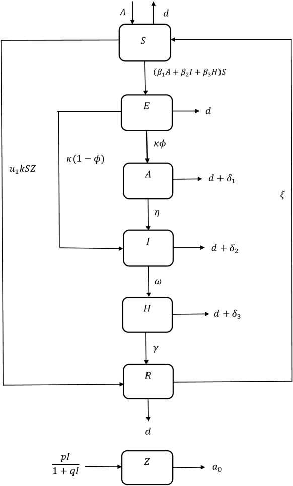
Schematic diagram of system (1)

Positivity and boundedness

For system (1): the following two theorems prove that the system variables are positive and bounded for all time.

Theorem 3.1

All solutions of system (1) starting from ${\mathbb{R}}_{+}^7$ remain positive for all the time.

Proof

Continuity and locally Lipschitzian functions of right-hand side of model (1) on C result in occurrence of a unique solution $(S(t),E(t),A(t),I(t),H(t),R(t),Z(t))$ on $[0,\tau ),$ where $0<\tau \le +\infty$ [21]. First we need to show that, $S(t)>0,\forall t\in [0,\tau )$. If it does not hold, then $\exists t_1\in (0,\tau )$ such that $S(t_1)=0,\dot{S}(t_1)\le 0$ and $S(t)>0,\forall t\in [0,t_1).$ Hence we must have $E(t)\ge 0,\forall t\in [0,t_1).$ If it is not true, then $\exists t_2\in (0,t_1)$ such that $E(t_2)=0,\dot{E}(t_2)<0$ and $E(t)\ge 0,\forall t\in [0,t_2).$ Next we claim $A(t)\ge 0,\forall t\in [0,t_2).$ Suppose it is not true. Then $\exists t_3\in (0,t_2)$ such that $A(t_3)=0,\dot{A}(t_3)<0$ and $A(t)\ge 0,\forall t\in [0,t_3).$ From third equation of (1), we have

$$\begin{array}{cc}\hfill \frac{\text{d}A}{\text{d}t}{|}_{t=t_3}=& \kappa \varphi E(t_3)-(\eta +d+{\delta }_1)A(t_3)\hfill \\ \hfill =& \kappa \varphi E(t_3)\ge 0,\hfill \end{array}$$

which is a contradiction to $\dot{A}(t_3)<0.$ So, $A(t)\ge 0,\forall t\in [0,t_2).$

Our next claim is $I(t)\ge 0,\forall t\in [0,t_2).$ If it is not true, then $\exists t_4\in (0,t_2)$ such that $I(t_4)=0,\dot{I}(t_4)<0$ and $I(t)\ge 0,\forall t\in [0,t_4).$ Now from the fourth equation of (1):

$$\begin{array}{cc}\hfill \frac{\text{d}I}{\text{d}t}{|}_{t=t_4}=& \kappa (1-\varphi )I(t_4)+\eta I(t_4)\hfill \\ \hfill & -(\omega +d+{\delta }_2)I(t_4)\hfill \\ \hfill =& \kappa (1-\varphi )I(t_4)+\eta I(t_4)\ge 0,\hfill \end{array}$$

which is a contradiction to $\dot{I}(t_4)<0.$ Hence, $I(t)\ge 0,\forall t\in [0,t_2).$

Next claim is $H(t)\ge 0,\forall t\in [0,t_2).$ Let the statement is not true. Then $\exists t_5\in (0,t_2)$ such that $H(t_5)=0,\dot{H}(t_5)<0$ and $H(t)\ge 0,\forall t\in [0,t_5).$ From the fifth equation of (1), we have

$$\begin{array}{c}\hfill \begin{array}{cc}\hfill \frac{\text{d}H}{\text{d}t}{|}_{t=t_5}& =\omega I(t_5)-(\gamma +d+{\delta }_3)H(t_5)\hfill \\ \hfill & =\omega I(t_5)\ge 0,\hfill \end{array}\end{array}$$

which is a contradiction to $\dot{H}(t_5)<0.$ So, $H(t)\ge 0,\forall t\in [0,t_2).$ From the second equation of (1):

$$\begin{array}{c}\hfill \begin{array}{cc}\hfill \frac{\text{d}E}{\text{d}t}{|}_{t=t_2}& =({\beta }_{1}A(t_2)+{\beta }_{2}I(t_2)+{\beta }_{3}H(t_2))S(t_2)\hfill \\ \hfill & \ge 0[\because E(t_2)=0].\hfill \end{array}\end{array}$$

It is a contradiction to $\dot{E}(t_2)<0.$ So, $E(t)\ge 0,\forall t\in [0,t_1).$ Hence $A(t)\ge 0,I(t)\ge 0,H(t)\ge 0,\forall t\in [0,t_1).$

Proceeding as before, it can be proved that $Z(t)\ge 0,R(t)\ge 0,\forall t\in [0,t_1).$

From the first equation of (1), we have

$$\begin{array}{c}\hfill \begin{array}{cc}\hfill \frac{\text{d}S}{\text{d}t}{|}_{t=t_1}& =\mathrm{\Lambda }+\xi R(t_1)>0[\because S(t_1)=0],\hfill \end{array}\end{array}$$

which is a contradiction to $\dot{S}(t_1)\le 0.$ So, $S(t)>0,\forall t\in [0,\tau ),$ where $0<\tau \le +\infty$. Also, by the previous steps we have $E(t)\ge 0,A(t)\ge 0,I(t)\ge 0,H(t)\ge 0,R(t)\ge 0$ and $Z(t)\ge 0,\forall t\in [0,\tau ),$ where $0<\tau \le +\infty .$ Hence proved. $\square$

Theorem 3.2

Solutions of system (1) which start from ${\mathbb{R}}_{+}^7$ remain uniformly bounded for all the time.

Proof

$$\begin{array}{c}\hfill \begin{array}{cc}\hfill \text{Let},N(t)& =S(t)+E(t)+A(t)+I(t)+H(t)+R(t)\hfill \\ \hfill \therefore \frac{\text{d}N}{\text{d}t}& =\mathrm{\Lambda }-dN\hfill \\ \hfill \Rightarrow 0& <N(t)\le N(0)e^{-dt}+\frac{\mathrm{\Lambda }}{d}\left(1,-,e^{-dt}\right)\hfill \end{array}\end{array}$$

where $N(0)=S(0)+E(0)+A(0)+I(0)+H(0)+R(0)$.

As ${\displaystyle t\to \infty ,0<N(t)\le \frac{\mathrm{\Lambda }}{d}.}$ From the last equation of system (1), we have

$$\begin{array}{c}\hfill \begin{array}{cc}\hfill \frac{\text{d}Z}{\text{d}t}& =\frac{\mathit{pI}}{1+qI}-a_{0}Z\le pI-a_{0}Z\hfill \\ \hfill \Rightarrow & \frac{\text{d}Z}{\text{d}t}+a_{0}Z\le \frac{p\mathrm{\Lambda }}{d}(\text{for large time}t).\hfill \\ \hfill \Rightarrow 0& <Z(t)\le Z(0)e^{-a_{0}t}+\frac{p\mathrm{\Lambda }}{a_{0}d}\left(1,-,e^{-a_{0}t}\right)\hfill \end{array}\end{array}$$

As ${\displaystyle t\to \infty ,0<Z(t)\le \frac{p\mathrm{\Lambda }}{a_{0}d}.}$

Hence, all solutions of system (1) enter in the region:

$$\begin{array}{cc}\hfill \mathrm{\Omega }=& \left\{(S,E,A,I,H,R,Z),\in ,{\mathbb{R}}_{+}^7,:,0,\le ,N,(t),\le ,\frac{\mathrm{\Lambda }}{d},;\right)\hfill \\ \hfill & \left(0,<,Z,(t),\le ,\frac{p\mathrm{\Lambda }}{a_{0}d}\right\}.\hfill \end{array}$$

$\square$

Equilibrium analysis

Here, we obtain the equilibrium points of system (1) by solving the isoclines and determine the basic reproduction number $R_0$ to determine existence of endemic equilibrium point. System (1) has following equilibrium points:

1. Disease-free equilibrium point (DFE): ${\displaystyle E_0(S_0,0,0,0,0,0,0)=\left(\frac{\mathrm{\Lambda }}{d},,,0,,,0,,,0,,,0,,,0,,,0\right)}$.

2. Endemic equilibrium point: $E^{\ast }(S^{\ast },E^{\ast },A^{\ast },I^{\ast },H^{\ast },R^{\ast },Z^{\ast })$.

Basic reproduction number $(R_0)$

Basic reproduction number $R_0$ basically is a threshold value which denotes the average number of newly infected individuals after coming in contact with a single infected individual in a susceptible population. A method was developed by van den Driessche and Watmough [39] which is used here to determine the basic reproduction number. In system (1), people move into exposed class when the disease is introduced and also the infected classes are asymptomatic (A), symptomatic stages (I) and hospitalised stage (H). Let us take $x\equiv (E,A,I,H)$. Second, third, fourth and fifth equations of model (1) is written as:

$$\begin{array}{cc}\hfill \frac{\text{d}x}{\text{d}t}=& \mathfrak{F}(x)-\nu (x),\hfill \\ \hfill \mathfrak{F}(x)=& \left(\begin{array}{c}({\beta }_{1}A+{\beta }_{2}I+{\beta }_{3}H)S\\ 0\\ 0\\ 0\end{array}\right),\hfill \\ \hfill \nu (x)=& \left(\begin{array}{c}(\kappa +d)E\\ -\kappa \varphi E+(\eta +d+{\delta }_1)A\\ -\kappa (1-\varphi )E-\eta A+(\omega +d+{\delta }_2)I\\ -\omega I+(\gamma +d+{\delta }_3)H\end{array}\right),\hfill \end{array}$$

where $\mathfrak{F}(x)$ contains only that compartment where new infection term is introduced and $\nu (x)$ contains rest of the terms. So, corresponding linearised matrices of $\mathfrak{F}(x)$ and $\nu (x)$ at disease-free equilibrium $E_0=(S_0,0,0,0,0,0,0)$ are, respectively

$$\begin{array}{cc}\hfill F=& \left(D,\mathfrak{F},(,x,)\right)(E_0)=\left(\begin{array}{cccc}0& {\beta }_1{S}_0& {\beta }_2{S}_0& {\beta }_3{S}_0\\ 0& 0& 0& 0\\ 0& 0& 0& 0\\ 0& 0& 0& 0\end{array}\right),\hfill \\ \hfill V=& \left(D,\nu ,(,x,)\right)(E_0)\hfill \\ \hfill =& \left(\begin{array}{cccc}\kappa +d& 0& 0& 0\\ -\kappa \varphi & \eta +d+{\delta }_1& 0& 0\\ -\kappa (1-\varphi )& -\eta & \omega +d+{\delta }_2& 0\\ 0& 0& -\omega & \gamma +d+{\delta }_3\end{array}\right)\hfill \end{array}$$

Let, ${\alpha }_0=\kappa +d,{\alpha }_1=\eta +d+{\delta }_1,{\alpha }_2=\omega +d+{\delta }_2,{\alpha }_3=\gamma +d+{\delta }_3$.

Here, $|V|=det(V)=(\kappa +d)(\eta +d+{\delta }_1)(\omega +d+{\delta }_2)(\gamma +d+{\delta }_3)={\alpha }_0{\alpha }_1{\alpha }_2{\alpha }_3$.

As the spectral radius of the next generation matrix $F{V}^{-1}$ is $R_0$, then the basic reproduction number of system (1) is given by [39]:

$$\begin{array}{c}\hfill \begin{array}{cc}\hfill R_0& =\frac{\kappa S_0}{|V|}\hfill \\ \hfill & [{\beta }_1\varphi {\alpha }_2{\alpha }_3+({\beta }_2{\alpha }_3+{\beta }_3\omega )\{\varphi \eta +{\alpha }_1(1-\varphi )\}]\hfill \\ \hfill & =\frac{\kappa \mathrm{\Lambda }}{d{\alpha }_0{\alpha }_1{\alpha }_2{\alpha }_3}\hfill \\ \hfill & [{\beta }_1\varphi {\alpha }_2{\alpha }_3+({\beta }_2{\alpha }_3+{\beta }_3\omega )\{\varphi \eta +{\alpha }_1(1-\varphi )\}]\hfill \end{array}\\ \hfill \end{array}$$ 2

Existence of endemic equilibrium point $E^{\ast }(S^{\ast },E^{\ast },A^{\ast },I^{\ast },H^{\ast },R^{\ast },Z^{\ast })$

From system (1):

$$\begin{array}{c}\hfill \begin{array}{cc}& \mathrm{\Lambda }-({\beta }_1{A}^{\ast }+{\beta }_2{I}^{\ast }+{\beta }_3{H}^{\ast })S^{\ast }-d{S}^{\ast }\hfill \\ \hfill & +\xi R^{\ast }-u_{1}k{S}^{\ast }{Z}^{\ast }=0,\hfill \\ \hfill & ({\beta }_1{A}^{\ast }+{\beta }_2{I}^{\ast }+{\beta }_3{H}^{\ast })S-(\kappa +d)E^{\ast }=0,\hfill \\ \hfill & \kappa \varphi E^{\ast }-(\eta +d+{\delta }_1)A^{\ast }=0,\hfill \\ \hfill & \kappa (1-\varphi )E^{\ast }+\eta A^{\ast }-(d+{\delta }_2+\omega )I^{\ast }=0,\hfill \\ \hfill & \omega I^{\ast }-(\gamma +d+{\delta }_3)H^{\ast }=0,\hfill \\ \hfill & \gamma H^{\ast }-(d+\xi )R^{\ast }+u_{1}k{S}^{\ast }{Z}^{\ast }=0,\hfill \\ \hfill & \frac{p{I}^{\ast }}{1+q{I}^{\ast }}-a_0{Z}^{\ast }\hfill & \hfill =0.\end{array}\end{array}$$ 3

Solving these equations, we get

$$\begin{array}{cc}\hfill S^{\ast }=& \frac{\mathrm{\Lambda }}{d{R}_0},Z^{\ast }=\frac{p{I}^{\ast }}{a_0(1+q{I}^{\ast })},\hfill \\ \hfill H^{\ast }=& \frac{\omega I^{\ast }}{{\alpha }_3},E^{\ast }=\frac{{\alpha }_1{\alpha }_2{I}^{\ast }}{\kappa \{\varphi \eta +{\alpha }_1(1-\varphi )\}},\hfill \\ \hfill A^{\ast }=& \frac{\varphi {\alpha }_2{I}^{\ast }}{\{\varphi \eta +{\alpha }_1(1-\varphi )\}},\hfill \\ \hfill R^{\ast }=& \frac{[\gamma \omega d{a}_0{R}_0(1+q{I}^{\ast })+u_{1}kp\mathrm{\Lambda }{\alpha }_3]I^{\ast }}{a_{0}d{R}_0{\alpha }_3(d+\xi )(1+q{I}^{\ast })}\hfill \end{array}$$

and $I^{\ast }$ is a positive root of the equation:

$$\begin{array}{c}\hfill P_1{I}^2+P_{2}I+P_3=0,\end{array}$$

where

$$\begin{array}{c}\hfill \begin{array}{cc}& P_1=q\left[\frac{\gamma \xi \omega }{{\alpha }_3(d+\xi )},-,\frac{{\alpha }_0{\alpha }_1{\alpha }_2}{\kappa \{\varphi \eta +{\alpha }_1(1-\varphi )\}}\right]\hfill \\ \hfill & =-\frac{q[{\alpha }_1\{d{\alpha }_0{\alpha }_1{\alpha }_2+\xi d{\alpha }_2{\alpha }_3+\kappa \xi {\alpha }_3(d+{\delta }_2)+\xi \kappa \omega (d+{\delta }_3)\}+\varphi \gamma \xi \omega \kappa (d+{\delta }_1)]}{\kappa {\alpha }_3(d+\xi )\{\varphi \eta +{\alpha }_1(1-\varphi )\}}<0\hfill \\ \hfill & P_2=q\mathrm{\Lambda }\left(1,-,\frac{1}{R_0}\right)+\left[\frac{\gamma \xi \omega }{{\alpha }_3(d+\xi )},-,\frac{{\alpha }_0{\alpha }_1{\alpha }_2}{\kappa \{\varphi \eta +{\alpha }_1(1-\varphi )\}}\right]-\frac{u_{1}kp\mathrm{\Lambda }}{a_0{R}_0(d+\xi )},\hfill \\ \hfill & P_3=\mathrm{\Lambda }\left(1,-,\frac{1}{R_0}\right)\hfill \end{array}\end{array}$$

Here, $P_3>0$ when $R_0>1$. As $P_1$ is always negative, so, for $R_0>1,$ we get a unique endemic equilibrium point. But when $R_0<1$, both of $P_2$ and $P_3$ become negative resulting in non-occurrence of an endemic equilibrium. Hence we have the following theorem.

Theorem 4.1

System (1) has a disease-free equilibrium point $E_0\left(S_0,,,0,,,0,,,0,,,0,,,0,,,0\right)$ for any parametric values. And for $R_0>1,$ the system possesses a unique endemic equilibrium $E^{\ast }(S^{\ast },E^{\ast },A^{\ast },I^{\ast },H^{\ast },R^{\ast },Z^{\ast }).$

Sensitivity analysis

For system (1), $R_0$ depends on some of the vital parameters such as recruitment rate $(\mathrm{\Lambda })$, transmission rates $({\beta }_1,{\beta }_2,{\beta }_3),$ disease related death rates $({\delta }_1,{\delta }_2,{\delta }_3)$, natural death rate (d), progression rate of exposed people into infected classes $(\kappa )$, probability at which exposed people move into infected classes $(\varphi )$, progression rate of asymptomatic infected individual into symptomatic class $(\eta )$, progression rate of symptomatic infected population into treatment class $(\omega )$, progression rate of hospitalised population into recovered class $(\gamma )$. But among all these parameters, we cannot control only ${\beta }_1,{\beta }_2,{\beta }_3,\kappa ,\omega .$

Now, ${\displaystyle R_0=\frac{\kappa \mathrm{\Lambda }}{d{\alpha }_0{\alpha }_1{\alpha }_2{\alpha }_3}[{\beta }_1\varphi {\alpha }_2{\alpha }_3+({\beta }_2{\alpha }_3+{\beta }_3\omega )\{\varphi \eta +{\alpha }_1(1-\varphi )\}],}$ where ${\alpha }_0=\kappa +d,{\alpha }_1=\eta +d+{\delta }_1,{\alpha }_2=\omega +d+{\delta }_2$ and ${\alpha }_3=\gamma +d+{\delta }_3$. From the expression of $R_0$:

$$\begin{array}{c}\hfill \begin{array}{cc}\hfill \frac{\partial R_0}{\partial {\beta }_1}& =\frac{\mathrm{\Lambda }\kappa \varphi }{d{\alpha }_0{\alpha }_1}>0\hfill \\ \hfill \frac{\partial R_0}{\partial {\beta }_2}& =\frac{\mathrm{\Lambda }\kappa \{\varphi \eta +{\alpha }_1(1-\varphi )\}}{d{\alpha }_0{\alpha }_1{\alpha }_2}>0\hfill \\ \hfill \frac{\partial R_0}{\partial {\beta }_3}& =\frac{\mathrm{\Lambda }\kappa \omega \{\varphi \eta +{\alpha }_1(1-\varphi )\}}{d{\alpha }_0{\alpha }_1{\alpha }_2{\alpha }_3}>0\hfill \\ \hfill \frac{\partial R_0}{\partial \kappa }& =\frac{\mathrm{\Lambda }[{\beta }_1\varphi {\alpha }_2{\alpha }_3+({\beta }_2{\alpha }_3+{\beta }_3\omega )\{\varphi \eta +{\alpha }_1(1-\varphi )\}]}{{\alpha }_0^2{\alpha }_1{\alpha }_2{\alpha }_3}\hfill \\ \hfill & >0\hfill \\ \hfill \frac{\partial R_0}{\partial \omega }& =\frac{\mathrm{\Lambda }\kappa \{\varphi \eta +{\alpha }_1(1-\varphi )\}}{d{\alpha }_0{\alpha }_1{\alpha }_2^2{\alpha }_3}\hfill \\ \hfill & [{\beta }_3(d+{\delta }_2)-{\beta }_2(\gamma +d+{\delta }_3)]\hfill \end{array}\end{array}$$

So, ${\displaystyle \frac{\partial R_0}{\partial \omega }}$ is monotonic decreasing when ${\beta }_3(d+{\delta }_2)<{\beta }_2(\gamma +d+{\delta }_3)$ holds. Next we compute normalised forward sensitivity index with respect to each of the parameters ${\beta }_1,{\beta }_2,{\beta }_3,\kappa$ and $\omega$ to analyse the sensitivity of $R_0$ (to each of the parameters) by the method of Arriola and Hyman [1]:

$$\begin{array}{cc}\hfill {\mathrm{\Gamma }}_{{\beta }_1}=& \left|\frac{\frac{\partial R_0}{R_0}}{\frac{\partial {\beta }_1}{{\beta }_1}}\right|=\left|\frac{{\beta }_1}{R_0},\frac{\partial R_0}{\partial {\beta }_1}\right|\hfill \\ \hfill =& \left|\frac{{\beta }_1\varphi {\alpha }_2{\alpha }_3}{[{\beta }_1\varphi {\alpha }_2{\alpha }_3+({\beta }_2{\alpha }_3+{\beta }_3\omega )\{\varphi \eta +{\alpha }_1(1-\varphi )\}]}\right|<1\hfill \\ \hfill {\mathrm{\Gamma }}_{{\beta }_2}=& \left|\frac{\frac{\partial R_0}{R_0}}{\frac{\partial {\beta }_2}{{\beta }_2}}\right|=\left|\frac{{\beta }_2}{R_0},\frac{\partial R_0}{\partial {\beta }_2}\right|\hfill \\ \hfill =& \left|\frac{{\beta }_2{\alpha }_3\{\varphi \eta +{\alpha }_1(1-\varphi )\}}{[{\beta }_1\varphi {\alpha }_2{\alpha }_3+({\beta }_2{\alpha }_3+{\beta }_3\omega )\{\varphi \eta +{\alpha }_1(1-\varphi )\}]}\right|<1\hfill \\ \hfill {\mathrm{\Gamma }}_{{\beta }_3}=& \left|\frac{\frac{\partial R_0}{R_0}}{\frac{\partial {\beta }_3}{{\beta }_3}}\right|=\left|\frac{{\beta }_3}{R_0},\frac{\partial R_0}{\partial {\beta }_3}\right|\hfill \\ \hfill =& \left|\frac{{\beta }_3\omega \{\varphi \eta +{\alpha }_1(1-\varphi )\}}{[{\beta }_1\varphi {\alpha }_2{\alpha }_3+({\beta }_2{\alpha }_3+{\beta }_3\omega )\{\varphi \eta +{\alpha }_1(1-\varphi )\}]}\right|<1\hfill \\ \hfill {\mathrm{\Gamma }}_{\kappa }=& \left|\frac{\frac{\partial R_0}{R_0}}{\frac{\partial \kappa }{\kappa }}\right|=\left|\frac{\text{d}}{\kappa +d}\right|<1\hfill \\ \hfill {\mathrm{\Gamma }}_{\omega }=& \left|\frac{\frac{\partial R_0}{R_0}}{\frac{\partial \omega }{\omega }}\right|=\left|\frac{\omega }{R_0},\frac{\partial R_0}{\partial \omega }\right|\hfill \\ \hfill =& \left|\frac{\omega \{\varphi \eta +{\alpha }_1(1-\varphi )\}\{{\beta }_3(d+{\delta }_2)-{\beta }_2(\gamma +d+{\delta }_3)\}}{{\alpha }_2[{\beta }_1\varphi {\alpha }_2{\alpha }_3+({\beta }_2{\alpha }_3+{\beta }_3\omega )\{\varphi \eta +{\alpha }_1(1-\varphi )\}]}\right|\hfill \end{array}$$

From the calculation, it is observed that the disease transmission rates from asymptomatically infected $({\beta }_1)$, symptomatically infected $({\beta }_2)$ and hospitalised individuals $({\beta }_3)$ maintain direct proportional relation with basic reproduction number which is biologically acceptable too. Increasing disease transmission rates can stimulate the probability of occurrence of an epidemic outbreak. Moreover, if more people from the exposed class move into infected classes whether in asymptomatic stage or symptomatic stage, then the chance of getting an infected system increase. The calculation also shows that $R_0$ increases for increasing value of $\kappa$. On the other hand, $\omega$ denotes the rate at which the symptomatically infected individuals are admitted to hospitals for treatment. So, it is evident that increasing $\omega$ helps to reduce the disease prevalence and hence $\omega$ maintains an inversely proportional relation with $R_0$, i.e. increment in this parameter leads to a decrease in $R_0$. Here, ${\displaystyle \frac{\partial R_0}{\partial \omega }<0}$ only when ${\beta }_3(d+{\delta }_2)<{\beta }_2(\gamma +d+{\delta }_3)$ holds. So, maintaining this inequality can reduce the disease outbreak for increasing hospitalisation rate. The calculations and numerical simulations reveal that $R_0$ is more sensitive to changes in ${\beta }_i$ for $i=1,2,3$ than $\kappa$ and $\omega$. So, if we try to reduce the transmission rates by maintaining social distances and taking proper precautions, then this epidemic situation may be handled.

Stability analysis

We discuss the local and global stability conditions for the disease-free equilibrium point as well as endemic equilibrium point in this section. Let, ${\alpha }_0=d+\kappa ,{\alpha }_1=\eta +d+{\delta }_1,{\alpha }_2=\omega +d+{\delta }_2$ and ${\alpha }_3=\gamma +d+{\delta }_3$. The Jacobian matrix of system (1) is given as:

$$\begin{array}{cc}& \overline{J}\hfill \\ \hfill & =\left(\begin{array}{ccccccc}{a}_{11}& 0& -{\beta }_{1}S& -{\beta }_{2}S& -{\beta }_{3}S& \xi & -u_{1}kS\\ {\beta }_{1}A+{\beta }_{2}I+{\beta }_{3}H& -{\alpha }_0& {\beta }_{1}S& {\beta }_{2}S& {\beta }_{3}S& 0& 0\\ 0& \kappa \varphi & -{\alpha }_1& 0& 0& 0& 0\\ 0& \kappa (1-\varphi )& \eta & -{\alpha }_2& 0& 0& 0\\ 0& 0& 0& \omega & -{\alpha }_3& 0& 0\\ u_{1}kZ& 0& 0& 0& \gamma & -(d+\xi )& u_{1}kS\\ 0& 0& 0& \frac{p}{{(1+qI)}^2}& 0& 0& -a_0\end{array}\right)\hfill \\ \hfill \end{array}$$ 4

where $a_{11}=-({\beta }_{1}A+{\beta }_{2}I+{\beta }_{3}H)-d-u_{1}kZ.$

Local stability of $E_0$

Jacobian matrix at the disease-free equilibrium point ${\displaystyle E_0=\left(\frac{\mathrm{\Lambda }}{d},,,0,,,0,,,0,,,0,,,0,,,0\right)}$ is given as follows ${\displaystyle \left(S_0,=,\frac{\mathrm{\Lambda }}{d}\right)}$:

$$\begin{array}{c}\hfill \overline{J}{|}_{E_0}=\left(\begin{array}{ccccccc}-d& 0& -{\beta }_1{S}_0& -{\beta }_2{S}_0& -{\beta }_3{S}_0& \xi & -u_{1}k{S}_0\\ 0& -{\alpha }_0& {\beta }_1{S}_0& {\beta }_2{S}_0& {\beta }_3{S}_0& 0& 0\\ 0& \kappa \varphi & -{\alpha }_1& 0& 0& 0& 0\\ 0& \kappa (1-\varphi )& \eta & -{\alpha }_2& 0& 0& 0\\ 0& 0& 0& \omega & -{\alpha }_3& 0& 0\\ 0& 0& 0& 0& \gamma & -(d+\xi )& u_{1}k{S}_0\\ 0& 0& 0& p& 0& 0& -a_0\end{array}\right)\end{array}$$

Some of the eigenvalues of the Jacobian matrix $\overline{J}{|}_{E_0}$ are ${\lambda }_1=-d,{\lambda }_2=-(d+\xi ),{\lambda }_3=-a_0$ and other four eigenvalues are obtained from the roots of the following equation: ${\lambda }^4+Q_1{\lambda }^3+Q_2{\lambda }^2+Q_3\lambda +Q_4=0,$

where, $Q_1={\alpha }_0+{\alpha }_1+{\alpha }_2+{\alpha }_3$, $Q_2={\alpha }_0{\alpha }_1+{\alpha }_2{\alpha }_3+({\alpha }_0+{\alpha }_1)({\alpha }_2+{\alpha }_3)-\kappa S_0\{{\beta }_1\varphi +{\beta }_2(1-\varphi )\}$, $Q_3={\alpha }_0{\alpha }_1({\alpha }_2+{\alpha }_3)+{\alpha }_2{\alpha }_3({\alpha }_0+{\alpha }_1)-S_0\kappa [{\beta }_1\varphi ({\alpha }_2+{\alpha }_3)+{\beta }_2\{\varphi \eta +{\alpha }_1(1-\varphi )\}+({\beta }_2{\alpha }_3+{\beta }_3\omega )(1-\varphi )]$ and $Q_4={\alpha }_0{\alpha }_1{\alpha }_2{\alpha }_3(1-R_0)$. So, $Q_4>0$ for $R_0<1$. So for $R_0<1$, the characteristic equation has roots with negative real parts only when $Q_2,Q_3>0$ and we have the following theorem

Theorem 6.1

The DFE $(E_0)$ is locally asymptomatically stable (LAS) for $R_0<1$ when $Q_2>0$ and $Q_3>0$ hold.

Global stability of $E_0$

Theorem 6.2

DFE $E_0$ of system (1) is globally asymptotically stable (GAS) when $p<d$ and $u_{1}k\mathrm{\Lambda }<a_{0}d$ hold.

Proof

Let us consider the Lyapunov function as

$$\begin{array}{cc}\hfill V_1=& \left(S,-,S_0,-,S_0,l,n,\left(\frac{S}{S_0}\right)\right)\hfill \\ \hfill & +E+A+I+H+R+Z\hfill \end{array}$$

Here, $V_1$ is a positive definite function for all $(S,E,A,I,H,R,Z)$ other than the DFE. Time derivative of $V_1$ computed along the solutions of system (1) is given as:

$$\begin{array}{c}\hfill \begin{array}{cc}\hfill \frac{\text{d}{V}_1}{\text{d}t}& =\left(1,-,\frac{S_0}{S}\right)\hfill \\ \hfill & [\mathrm{\Lambda }-({\beta }_{1}A+{\beta }_{2}I+{\beta }_{3}H)S-dS+\xi R-u_{1}kSZ]\hfill \\ \hfill & +({\beta }_{1}A+{\beta }_{2}I+{\beta }_{3}H)S\hfill \\ \hfill & -d(E+A+I+H+R)-{\delta }_{1}A-{\delta }_{2}I\hfill \\ \hfill & -{\delta }_{3}H-\xi R+u_{1}kSZ+\frac{\mathit{pI}}{1+qI}-a_{0}Z\hfill \\ \hfill & =\mathrm{\Lambda }-d(E+A+I+H+R)-{\delta }_{1}A-{\delta }_{2}I\hfill \\ \hfill & -{\delta }_{3}H-\frac{\mathrm{\Lambda }{S}_0}{S}+d{S}_0-\frac{\xi S_{0}R}{S}\hfill \\ \hfill & +u_{1}k{S}_{0}Z+\frac{\mathit{pI}}{1+qI}-a_{0}Z\hfill \\ \hfill & \le \left(\frac{\mathrm{\Lambda }}{S},-,d\right)(S-S_0)+(p-d)I\hfill \\ \hfill & +\frac{1}{d}(u_{1}k\mathrm{\Lambda }-a_{0}d)Z\hfill \\ \hfill & =-\frac{\text{d}}{S}{(S-S_0)}^2+(p-d)I\hfill \\ \hfill & +\frac{1}{d}(u_{1}k\mathrm{\Lambda }-a_{0}d)Z\hfill \end{array}\end{array}$$

Hence, ${\displaystyle \frac{\text{d}{V}_1}{\text{d}t}<0}$ when $p<d$ and $u_{1}k\mathrm{\Lambda }<a_{0}d$ hold. Also, $\frac{\text{d}{V}_1}{\text{d}t}=0$ when $S=S_0$ and $E=A=I=H=R=Z=0.$ By LaSalle’s invariance principle [27], $E_0$ is globally asymptotically stable when $R_0<1$ when the mentioned parametric restrictions are fulfilled. $\square$

Local stability of $E^{\ast }$

Theorem 6.3

The endemic equilibrium point $E^{\ast }$ is LAS for $R_0>1$ when the conditions if $R_i>0$ for $i=1,7$ and ${\mathrm{\Delta }}_i>0$ for $i=2,3,4,5,6$ hold.

Proof

Proof is given in the “Appendix”. $\square$

Global stability of $E^{\ast }$

Theorem 6.4

The endemic equilibrium point $E^{\ast }$ of system (1) is globally asymptomatically stable (GAS) in

$$\begin{array}{c}\hfill \begin{array}{cc}\hfill \mathrm{\Phi }& =\left\{(S,E,A,I,H,R,A),\in ,{\mathbb{R}}_{+}^7,:\right)\hfill \\ \hfill & {(m_2{\beta }_{1}S)}^2<\frac{4}{9}{m}_2{\alpha }_0\hfill \\ \hfill & ({\delta }_1+m_3{\alpha }_1),{(m_2{\beta }_{3}S-{\delta }_3)}^2\hfill \\ \hfill & <\frac{1}{6}{m}_2{\delta }_3{\alpha }_3,\hfill \\ \hfill & {(m_2{\beta }_{2}S+m_4\kappa \varphi )}^2\hfill \\ \hfill & <\frac{m_2{\alpha }_0}{3}({\delta }_2+m_4{\alpha }_2),\hfill \\ \hfill & \left(\text{with},,(,i,),-,(,i,i,i,),,\text{as stated at the end in the proof}\right\},\hfill \end{array}\end{array}$$

where ${\alpha }_i$ for $i=0,1,2,3$ and $m_j$ for $j=1,2,3,4$ are mentioned in the proof.

Proof

Consider a Lyapunov function $V_2$ as:

$$\begin{array}{c}\hfill \begin{array}{cc}\hfill V_2(t)& =\frac{1}{2}[(S-S^{\ast })+(E-E^{\ast })+(A-A^{\ast })\hfill \\ \hfill & +(I-I^{\ast })+(H-H^{\ast })+(R-R^{\ast }){]}^2+\hfill \\ \hfill & \frac{m_1}{2}{(S-S^{\ast })}^2+\frac{m_2}{2}{(E-E^{\ast })}^2\hfill \\ \hfill & +\frac{m_3}{2}{(A-A^{\ast })}^2+\frac{m_4}{2}{(I-I^{\ast })}^2\hfill \\ \hfill & +\frac{1}{2}{(Z-Z^{\ast })}^2\hfill \end{array}\end{array}$$

Time derivative of $V_2$ along the solutions of system (1) is given as:

$$\begin{array}{c}\hfill \begin{array}{cc}\hfill \frac{\text{d}{V}_2}{\text{d}t}& =[(S-S^{\ast })+(E-E^{\ast })+(A-A^{\ast })\hfill \\ \hfill & +(I-I^{\ast })+(H-H^{\ast })+(R-R^{\ast })]\hfill \\ \hfill & \frac{\text{d}}{\text{d}t}(S+E+A+I+H+R)+m_1(S-S^{\ast })\frac{\text{d}S}{\text{d}t}\hfill \\ \hfill & +m_2(E-E^{\ast })\frac{\text{d}E}{\text{d}t}\hfill \\ \hfill & +m_3(A-A^{\ast })\frac{\text{d}A}{\text{d}t}+m_4(I-I^{\ast })\frac{\text{d}I}{\text{d}t}\hfill \\ \hfill & +(Z-Z^{\ast })\frac{\text{d}Z}{\text{d}t}\hfill \end{array}\end{array}$$

Now steady state of system (1) at $E^{\ast }$ gives

$$\begin{array}{cc}& \mathrm{\Lambda }-({\beta }_1{A}^{\ast }+{\beta }_2{I}^{\ast }+{\beta }_3{H}^{\ast })S^{\ast }-d{S}^{\ast }\hfill \\ \hfill & +\xi R^{\ast }-u_{1}k{S}^{\ast }{Z}^{\ast }=0,\hfill \\ \hfill & ({\beta }_1{A}^{\ast }+{\beta }_2{I}^{\ast }+{\beta }_3{H}^{\ast })S-(\kappa +d)E^{\ast }=0,\hfill \\ \hfill & \kappa \varphi E^{\ast }-(\eta +d+{\delta }_1)A^{\ast }=0,\hfill \\ \hfill & \kappa (1-\varphi )E^{\ast }+\eta A^{\ast }-(d+{\delta }_2+\omega )I^{\ast }=0,\hfill \\ \hfill & \omega I^{\ast }-(\gamma +d+{\delta }_3)H^{\ast }=0,\hfill \\ \hfill & \gamma H^{\ast }-(d+\xi )R^{\ast }+u_{1}k{S}^{\ast }{Z}^{\ast }=0,\hfill \\ \hfill & \frac{p{I}^{\ast }}{1+q{I}^{\ast }}-a_0{Z}^{\ast }=0,\hfill \\ \hfill & \mathrm{\Lambda }-d(S^{\ast }+E^{\ast }+A^{\ast }+I^{\ast }+H^{\ast }+R^{\ast })\hfill \\ \hfill & -{\delta }_1{A}^{\ast }-{\delta }_2{I}^{\ast }-{\delta }_3{H}^{\ast }=0\hfill \end{array}$$

Consider ${\alpha }_0=\kappa +d,{\alpha }_1=\eta +d+{\delta }_1,{\alpha }_2=d+{\delta }_2+\omega ,{\alpha }_3=\gamma +d+{\delta }_3$. So, we have

$$\begin{array}{cc}\hfill \frac{\text{d}{V}_2}{\text{d}t}& =[(S-S^{\ast })+(E-E^{\ast })+(A-A^{\ast })\hfill \\ \hfill & +(I-I^{\ast })+(H-H^{\ast })+(R-R^{\ast })]\hfill \\ \hfill & [\mathrm{\Lambda }-d(S+E+A+I+H+R)-{\delta }_{1}A\hfill \\ \hfill & -{\delta }_{2}I-{\delta }_{3}H]\hfill \\ \hfill & +m_1(S-S^{\ast })[\mathrm{\Lambda }-dS+\xi R\hfill \\ \hfill & -({\beta }_{1}A+{\beta }_{2}I+{\beta }_{3}H)S-u_{1}kSZ]\hfill \\ \hfill & +m_2(E-E^{\ast })[({\beta }_{1}A+{\beta }_{2}I+{\beta }_{3}H)S-{\alpha }_{0}E]\hfill \\ \hfill & +m_3(A-A^{\ast })[\kappa \varphi E-{\alpha }_{1}A]\hfill \\ \hfill & +m_4(I-I^{\ast })[\kappa (1-\varphi )E+\eta A-{\alpha }_{2}I]\hfill \\ \hfill & +(Z-Z^{\ast })\left(\frac{\mathit{pI}}{1+qI},-,a_0,Z\right)\hfill \\ \hfill & =[(S-S^{\ast })+(E-E^{\ast })+(A-A^{\ast })+(I-I^{\ast })\hfill \\ \hfill & +(H-H^{\ast })+(R-R^{\ast })]\hfill \\ \hfill & [-d(S-S^{\ast })-d(E-E^{\ast })-(d+{\delta }_1)(A-A^{\ast })\hfill \\ \hfill & -(d+{\delta }_2)(I-I^{\ast })-(d+{\delta }_3)\hfill \\ \hfill & (H-H^{\ast })-d(R-R^{\ast })]\hfill \\ \hfill & +m_1(S-S^{\ast })\hfill \\ \hfill & [\mathrm{\Lambda }-({\beta }_{1}A+{\beta }_{2}I+{\beta }_{3}H)S-dS+\xi R-u_{1}kSZ]\hfill \\ \hfill & +m_2(E-E^{\ast })\hfill \\ \hfill & [({\beta }_{1}A+{\beta }_{2}I+{\beta }_{3}H)S-{\alpha }_{0}E]\hfill \\ \hfill & +m_3(A-A^{\ast })[\kappa \varphi E-{\alpha }_{1}A]+m_4(I-I^{\ast })\hfill \\ \hfill & [\kappa (1-\varphi )E+\eta A-{\alpha }_{2}I]+(Z-Z^{\ast })\hfill \\ \hfill & \left(\frac{\mathit{pI}}{1+qI},-,a_0,Z\right)\hfill \\ \hfill \frac{\text{d}{V}_2}{\text{d}t}& =[(S-S^{\ast })+(E-E^{\ast })+(A-A^{\ast })\hfill \\ \hfill & +(I-I^{\ast })+(H-H^{\ast })+(R-R^{\ast })]\hfill \\ \hfill & [-d(S-S^{\ast })-d(E-E^{\ast })-(d+{\delta }_1)(A-A^{\ast })\hfill \\ \hfill & -(d+{\delta }_2)(I-I^{\ast })\hfill \\ \hfill & -(d+{\delta }_3)(H-H^{\ast })-d(R-R^{\ast })]\hfill \\ \hfill & +m_1(S-S^{\ast })\hfill \\ \hfill & [-{\beta }_1(AS-A^{\ast }{S}^{\ast })-{\beta }_2(IS-I^{\ast }{S}^{\ast })\hfill \\ \hfill & -{\beta }_3(HS-H^{\ast }{S}^{\ast })-d(S-S^{\ast })\hfill \\ \hfill & +\xi (R-R^{\ast })-u_{1}k(SZ-S^{\ast }{Z}^{\ast })]\hfill \\ \hfill & +m_2(E-E^{\ast })\hfill \\ \hfill & [{\beta }_1(AS-A^{\ast }{S}^{\ast })+{\beta }_2(IS-I^{\ast }{S}^{\ast })\hfill \\ \hfill & +{\beta }_3(HS-H^{\ast }{S}^{\ast })-{\alpha }_0(E-E^{\ast })]\hfill \\ \hfill & +m_3(A-A^{\ast })\hfill \\ \hfill & [\kappa \varphi (E-E^{\ast })-{\alpha }_1(A-A^{\ast })]\hfill \\ \hfill & +m_4(I-I^{\ast })\hfill \\ \hfill & [\kappa (1-\varphi )(E-E^{\ast }+\eta (A-A^{\ast })-{\alpha }_2(I-I^{\ast })]\hfill \\ \hfill & +(Z-Z^{\ast })\hfill \\ \hfill & \left[\frac{p(I-I^{\ast })}{(1+qI)(1+q{I}^{\ast })},-,a_0,(Z-Z^{\ast })\right]\hfill \\ \hfill & =-d{(S-S^{\ast })}^2\hfill \\ \hfill & -d{[(E-E^{\ast })+(A-A^{\ast })+(I-I^{\ast })+(H-H^{\ast })]}^2\hfill \\ \hfill & -m_2{\alpha }_0{(E-E^{\ast })}^2\hfill \\ \hfill & -({\delta }_1+m_3{\alpha }_1){(A-A^{\ast })}^2\hfill \\ \hfill & -({\delta }_2+m_4{\alpha }_2){(I-I^{\ast })}^2\hfill \\ \hfill & -{\delta }_3{(H-H^{\ast })}^2-d{(R-R^{\ast })}^2\hfill \\ \hfill & +[-2d+m_2({\beta }_1{A}^{\ast }+{\beta }_2{I}^{\ast }+{\beta }_3{H}^{\ast })]\hfill \\ \hfill & (S-S^{\ast })(E-E^{\ast })\hfill \\ \hfill & -[2d+{\delta }_1+m_1{\beta }_1{S}^{\ast }](S-S^{\ast })(A-A^{\ast })\hfill \\ \hfill & -[2d+{\delta }_2+m_1{\beta }_2{S}^{\ast }](S-S^{\ast })(I-I^{\ast })\hfill \\ \hfill & -[2d+{\delta }_3+m_1{\beta }_3{S}^{\ast }](S-S^{\ast })(H-H^{\ast })\hfill \\ \hfill & +(-2d+m_1\xi )(S-S^{\ast })(R-R^{\ast })\hfill \\ \hfill & +[-{\delta }_1+m_2{\beta }_{1}S+m_3\kappa \varphi ](E-E^{\ast })(A-A^{\ast })\hfill \\ \hfill & +[-{\delta }_2+m_2{\beta }_{2}S+m_4\kappa \varphi ](E-E^{\ast })(I-I^{\ast })\hfill \\ \hfill & +[-{\delta }_3+m_2{\beta }_{3}S](E-E^{\ast })(H-H^{\ast })\hfill \\ \hfill & -2d(E-E^{\ast })(R-R^{\ast })\hfill \\ \hfill & +[-({\delta }_1+{\delta }_2)+m_4\eta ](A-A^{\ast })(I-I^{\ast })\hfill \\ \hfill & -({\delta }_1+{\delta }_3)(A-A^{\ast })(H-H^{\ast })\hfill \\ \hfill & -{\delta }_1(A-A^{\ast })(R-R^{\ast })\hfill \\ \hfill & -({\delta }_2+{\delta }_3)(I-I^{\ast })(H-H^{\ast })\hfill \\ \hfill & -{\delta }_2(I-I^{\ast })(R-R^{\ast })\hfill \\ \hfill & -{\delta }_3(H-H^{\ast })(R-R^{\ast })\hfill \\ \hfill & +\frac{p(I-I^{\ast })(Z-Z^{\ast })}{(1+qI)(1+q{I}^{\ast })}-a_0{(Z-Z^{\ast })}^2\hfill \end{array}$$

Let, ${\displaystyle m_1=\frac{2d}{\xi },m_2=\frac{2d}{{\beta }_1{A}^{\ast }+{\beta }_2{I}^{\ast }+{\beta }_3{H}^{\ast }},m_3=\frac{{\delta }_1}{\kappa \varphi }}$ and ${\displaystyle m_4=\frac{{\delta }_1+{\delta }_2}{\eta }}$. Then we have

$$\begin{array}{c}\hfill \begin{array}{cc}\hfill \frac{\text{d}{V}_2}{\text{d}t}& =-d{(S-S^{\ast })}^2\hfill \\ \hfill & -d{[(E-E^{\ast })+(A-A^{\ast })+(I-I^{\ast })+(H-H^{\ast })]}^2\hfill \\ \hfill & -m_2{\alpha }_0{(E-E^{\ast })}^2\hfill \\ \hfill & -({\delta }_1+m_3{\alpha }_1){(A-A^{\ast })}^2\hfill \\ \hfill & -({\delta }_2+m_4{\alpha }_2){(I-I^{\ast })}^2\hfill \\ \hfill & -{\delta }_3{(H-H^{\ast })}^2-d{(R-R^{\ast })}^2\hfill \\ \hfill & -[2d+{\delta }_1+m_1{\beta }_1{S}^{\ast }](S-S^{\ast })(A-A^{\ast })\hfill \\ \hfill & -[2d+{\delta }_2+m_1{\beta }_2{S}^{\ast }](S-S^{\ast })(I-I^{\ast })\hfill \\ \hfill & -[2d+{\delta }_3+m_1{\beta }_3{S}^{\ast }](S-S^{\ast })(H-H^{\ast })\hfill \\ \hfill & +m_2{\beta }_{1}S(E-E^{\ast })(A-A^{\ast })\hfill \\ \hfill & +[-{\delta }_2+m_2{\beta }_{2}S+m_4\kappa \varphi ](E-E^{\ast })(I-I^{\ast })\hfill \\ \hfill & +[-{\delta }_3+m_2{\beta }_{3}S](E-E^{\ast })(H-H^{\ast })\hfill \\ \hfill & -2d(E-E^{\ast })(R-R^{\ast })\hfill \\ \hfill & -({\delta }_1+{\delta }_3)(A-A^{\ast })(H-H^{\ast })\hfill \\ \hfill & -{\delta }_1(A-A^{\ast })(R-R^{\ast })\hfill \\ \hfill & -({\delta }_2+{\delta }_3)(I-I^{\ast })(H-H^{\ast })\hfill \\ \hfill & -{\delta }_2(I-I^{\ast })(R-R^{\ast })-{\delta }_3(H-H^{\ast })(R-R^{\ast })\hfill \\ \hfill & +\frac{p(I-I^{\ast })(Z-Z^{\ast })}{(1+qI)(1+q{I}^{\ast })}-a_0{(Z-Z^{\ast })}^2\hfill \end{array}\end{array}$$

So, ${\displaystyle \frac{\text{d}{V}_2}{\text{d}t}<0}$ in $\mathrm{\Phi }$ when the following conditions hold:

• (i)${\displaystyle ({\delta }_1+m_3{\alpha }_1)>max\left\{\frac{3}{2d},{(2d+{\delta }_1+m_1{\beta }_1{S}^{\ast })}^2,,,\frac{9{\delta }_1^2}{4d}\right\}}$,
• (ii)${\displaystyle ({\delta }_2+m_4{\alpha }_2)>max\left\{\frac{4}{d},{(2d+{\delta }_2+m_1{\beta }_2{S}^{\ast })}^2,,,\frac{12{\delta }_2^2}{d},,,,\frac{8{({\delta }_2+{\delta }_3)}^2}{{\delta }_3},,,,\frac{2p^4{d}^4}{a_0{(d+q\mathrm{\Lambda })}^4}\right\}}$,
• (iii)${\displaystyle \frac{48}{d}{(2d+{\delta }_3+m_1{\beta }_3{S}^{\ast })}^2<12{\delta }_3<d<\frac{m_2{\alpha }_0}{18}}$.

Moreover, ${\displaystyle \frac{\text{d}{V}_2}{\text{d}t}{|}_{E^{\ast }}=0}$. So, by Lyapunov LaSalle’s theorem [27], $E^{\ast }$ is GAS in the interior of $\mathrm{\Phi }$ when the mentioned restrictions are fulfilled. $\square$

Forward bifurcation at $R_0=1$

A unique endemic equilibrium point $E^{\ast }$ of system (1) exists when basic reproduction number ($R_0$) exceeds 1. Also, for $R_0$ less than unity, there is no endemic equilibrium point. Hence, there exists of a transcritical bifurcation around the disease-free equilibrium point $E_0$ when $R_0=1$.

Theorem 7.1

The system undergoes a transcritical bifurcation with respect to the bifurcation parameter ${\beta }_1$ around ${\displaystyle E_0(S_0,0,0,0,0,0,0)\equiv \left(\frac{\mathrm{\Lambda }}{d},,,0,,,0,,,0,,,0,,,0,,,0\right)}$ for $R_0=1$.

Proof

Consider the RHS of system (1) as: $g={(g_1,g_2,g_3,g_4,g_5,g_6,g_7)}^T$ where

$$\begin{array}{cc}\hfill g_1=& \mathrm{\Lambda }-({\beta }_{1}A+{\beta }_{2}I+{\beta }_{3}H)S-dS+\xi R-u_{1}kSZ;\hfill \\ \hfill g_2=& ({\beta }_{1}A+{\beta }_{2}I+{\beta }_{3}H)S-(\kappa +d)E;\hfill \\ \hfill g_3=& \kappa \varphi E-(\eta +d+{\delta }_1)A;\hfill \\ \hfill g_4=& \kappa (1-\varphi )E+\eta A-(d+{\delta }_2+\omega )I;\hfill \\ \hfill g_5=& \omega I-(\gamma +d+{\delta }_3)H;\hfill \\ \hfill g_6=& \gamma H-(d+\xi )R+u_{1}kSZ;\hfill \\ \hfill g_7=& \frac{\mathit{pI}}{1+qI}-a_{0}Z.\hfill \end{array}$$

For system (1), ${\displaystyle R_0=\frac{\kappa \mathrm{\Lambda }}{d{\alpha }_0{\alpha }_1{\alpha }_2{\alpha }_3}[{\beta }_1\varphi {\alpha }_2{\alpha }_3+({\beta }_2{\alpha }_3+{\beta }_3\omega )\{\varphi \eta +{\alpha }_1(1-\varphi )\}]}$, where ${\alpha }_0=d+\kappa ,{\alpha }_1=\eta +d+{\delta }_1,{\alpha }_2=\omega +d+{\delta }_2,{\alpha }_3=\gamma +d+{\delta }_3$.

$$\begin{array}{c}\hfill \overline{J}{|}_{E_0}=\left(\begin{array}{ccccccc}-d& 0& -{\beta }_1{S}_0& -{\beta }_2{S}_0& -{\beta }_3{S}_0& \xi & -u_{1}k{S}_0\\ 0& -{\alpha }_0& {\beta }_1{S}_0& {\beta }_2{S}_0& {\beta }_3{S}_0& 0& 0\\ 0& \kappa \varphi & -{\alpha }_1& 0& 0& 0& 0\\ 0& \kappa (1-\varphi )& \eta & -{\alpha }_2& 0& 0& 0\\ 0& 0& 0& \omega & -{\alpha }_3& 0& 0\\ 0& 0& 0& 0& \gamma & -(d+\xi )& u_{1}k{S}_0\\ 0& 0& 0& p& 0& 0& -a_0\end{array}\right)\end{array}$$

The eigenvalues are ${\lambda }_1=-d,{\lambda }_2=-(d+\xi ),{\lambda }_3=-a_0$ and other four eigenvalues are roots of the equation: ${\lambda }^4+Q_1{\lambda }^3+Q_2{\lambda }^2+Q_3\lambda +Q_4=0$,

where, $Q_1={\alpha }_0+{\alpha }_1+{\alpha }_2+{\alpha }_3$, $Q_2={\alpha }_0{\alpha }_1+{\alpha }_2{\alpha }_3+({\alpha }_0+{\alpha }_1)({\alpha }_2+{\alpha }_3)-\kappa S_0\{{\beta }_1\varphi +{\beta }_2(1-\varphi )\}$, $Q_3={\alpha }_0{\alpha }_1({\alpha }_2+{\alpha }_3)+{\alpha }_2{\alpha }_3({\alpha }_0+{\alpha }_1)-S_0\kappa [{\beta }_1\varphi ({\alpha }_2+{\alpha }_3)+{\beta }_2\{\varphi \eta +{\alpha }_1(1-\varphi )\}+({\beta }_2{\alpha }_3+{\beta }_3\omega )(1-\varphi )]$ and $Q_4={\alpha }_0{\alpha }_1{\alpha }_2{\alpha }_3(1-R_0)$.

Let ${\displaystyle {\beta }_{1[TC]}=\frac{1}{\varphi {\alpha }_2{\alpha }_3}\left[\frac{\text{d}{\alpha }_0{\alpha }_1{\alpha }_2{\alpha }_3}{\mathrm{\Lambda }\kappa },-,({\beta }_2{\alpha }_3+{\beta }_3\omega ),\{\varphi \eta +{\alpha }_1(1-\varphi )\}\right]}$ be the value of ${\beta }_1$ such that $R_0=1$ which implies $\overline{J}{|}_{E_0}$ has a simple zero eigenvalue at ${\beta }_1={\beta }_{1[TC]}.$ Also, $V={(v_1,v_2,v_3,v_4,v_5,v_6,v_7)}^T$ and $W={(w_1,w_2,w_3,w_4,w_5,w_6,w_7)}^T$, respectively, be the eigenvectors of ${\displaystyle \overline{J}{|}_{E_0}}$ and ${\displaystyle \overline{J}{|}_{E_0}^T}$ corresponding to the zero eigenvalue.

Calculations give ${\displaystyle v_1=\kappa (\xi \gamma \omega a_0-u_{1}k\mathrm{\Lambda }p{\alpha }_3)\{\varphi \eta +{\alpha }_1(1-\varphi )\}-a_0{\alpha }_0{\alpha }_1{\alpha }_2{\alpha }_3(d+\xi ),v_2=d{a}_0{\alpha }_0{\alpha }_1{\alpha }_2{\alpha }_3(d+\xi ),v_3=d\varphi a_0\kappa {\alpha }_2{\alpha }_3(d+\xi ),v_4=d{a}_0{\alpha }_3\kappa (d+\xi )\{\varphi \eta +{\alpha }_1(1-\varphi )\},v_5=\omega d{a}_0\kappa (d+\xi )\{\varphi \eta +{\alpha }_1(1-\varphi )\},v_6=\kappa \{\varphi \eta +{\alpha }_1(1-\varphi )\}(\gamma \omega a_{0}d+u_{1}k\mathrm{\Lambda }p{\alpha }_3)}$ and $v_7=pd{\alpha }_3\kappa (d+\xi )\{\varphi \eta +{\alpha }_1(1-\varphi )\}$. Also, $w_1=w_6=w_7=0,w_2=d{\alpha }_1{\alpha }_2{\alpha }_3,w_3=\mathrm{\Lambda }\{{\beta }_1{\alpha }_2{\alpha }_3+\eta ({\beta }_2{\alpha }_3+{\beta }_3\omega )\},w_4=\mathrm{\Lambda }{\alpha }_1({\beta }_2{\alpha }_3+{\beta }_3\omega )$ and $w_5=\mathrm{\Lambda }{\alpha }_1{\alpha }_2{\beta }_3$. Therefore,

$$\begin{array}{c}\hfill \begin{array}{cc}\hfill {\mathrm{\Omega }}_1& =W^T.g_{{\beta }_1}(E_0,{\beta }_{1[TC]})\hfill \\ \hfill & =w_2(AS){|}_{E_0}=0,\hfill \\ \hfill {\mathrm{\Omega }}_2& =W^T\left[D,g_{{\beta }_1},(E_0,{\beta }_{1[TC]}),V\right]\hfill \\ \hfill & =S_0{v}_3{w}_2\ne 0,\hfill \\ \hfill {\mathrm{\Omega }}_3& =W^T\left[D^2,g,(E_0,{\beta }_{1[TC]}),(V,V)\right]\hfill \\ \hfill & =2({\beta }_1{v}_3+{\beta }_2{v}_4+{\beta }_3{v}_5)v_1{w}_2\ne 0.\hfill \end{array}\end{array}$$

Thus, in view of Sotomayor’s Theorem, system (1) possesses a transcritical bifurcation around $E_0$ at $R_0=1$ taking ${\beta }_1$ as bifurcating parameter. $\square$

Numerical simulation without any control policy

Pictorial scenarios help us to understand system dynamics more clearly. The human population in India in April 2020 is about 136 million, the annual birth rate is 18.7 births/1000 people and the annual death rate is 7.3 deaths/1000 people. So, we are taking $S(0)=1.36\times {10}^9$ and $\mathrm{\Lambda }=7\times {10}^4$ by applying unit conversion from year to day. And the death rate per day we get is near about 0.00002. For the sake of calculation, we are taking $d=0.000055$. From the data provided in the dashboard by the centre for system science and engineering (CSSE) at John Hopkins University on 13th April 2020, India has 9352 corona activated cases [6]. And till the date, total death cases are 324 and recovered cases are 980. Hence, unit conversion to day gives ${\delta }_3$ as $8\times {10}^{-4}$ and $\xi$ as $3\times {10}^{-3}$. As total active cases till 13th is 8048 among 9352 cases; so, we get $\omega$ as 0.02 approximately [29]. According to the current epidemic situation of coronavirus, the new human cases infected per unit time is denoted by $\beta SI\equiv ({\beta }_{1}A+{\beta }_{2}I+{\beta }_{3}H)S$. Human cases infected by COVID-19 in March was (I) is about 1393, the population in India (S) in April is approximately by $1.35\times {10}^9$, the new human cases $({\beta }_{2}SI)$ till 13th April is about 9352 [29], hence we have ${\beta }_2\approx 1.5\times {10}^{-10}$ by doing the unit conversion from month to day. As per the data of March provided by Ministry of Health and Family Welfare, Government of India, the infected cases by COVID-19 is about 1393, so, for sake of simplicity I(0) is taken as 40. Now, all the assumed and estimated parameters are listed in Table 1. By CDC reports, mostly 25% of infected may not show any symptoms, i.e. remain as asymptomatic [7]. So, we have assumed $A(0)=10$. Also, $E(0)={10}^3,H(0)=15,R(0)=5$ and $Z(0)=0.5$ have been assumed.

Table 1.

Parameter values used for numerical simulation of system (1)

Parametric values
$\mathrm{\Lambda }$	$7\times {10}^4$	${\beta }_1$	$0.37\times {10}^{-10}$
${\beta }_2$	$1.48\times {10}^{-10}$	${\beta }_3$	$0.15\times {10}^{-10}$
$\xi$	$3\times {10}^{-10}$	$u_1$	0.1
k	0.002	$\kappa$	0.6
$\varphi$	0.1	$\eta$	0.15
${\delta }_1$	${10}^{-4}$	${\delta }_2$	$5\times {10}^{-4}$
${\delta }_3$	$8\times {10}^{-4}$	$\omega$	0.02
$\gamma$	0.5	d	0.000055
p	0.01	q	1
$a_0$	0.06

Figure 2 shows that for the parametric values in Table 1 and $d=0.6$, the trajectory starting from mentioned initial point ultimately converges to DFE $E_0(1.273\times {10}^9,0,0,0,0,0,0)$ and as we get the basic reproduction number $R_0$ as 0.000013 here which lies below unity, so, the disease cannot invade in the system in this case.

Fig. 2.

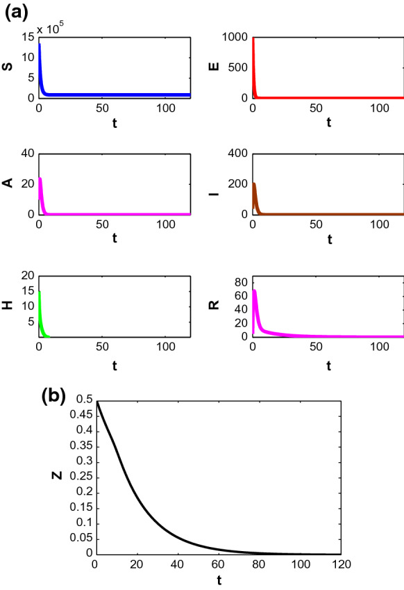
Stability of the populations around disease-free equilibrium $E_0$

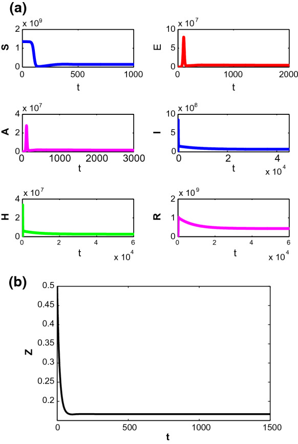
Now if we start to decrease the value of d, then for $d=0.000055$ along with parametric values in Table 1, the trajectory starting from mentioned initial point approaches to unique endemic equilibrium point $E^{\ast }(1.3788\times {10}^8,2.2419\times {10}^6,895850.6,6.5435\times {10}^7,2.6129\times {10}^6,4.2916\times {10}^8,0.1667)$ with time (see Fig. 3). For these parametric values we get $R_0=9.2305>1$ indicating the presence of infection in the system.

Fig. 3.

Stability of the populations around endemic equilibrium $E^{\ast }$

Now $E_0$ changes its stability when d comes below of a threshold value $d_{[TC]}$ and becomes stable for $d>d_{[TC]}$. So, the system undergoes a transcritical bifurcation at $d=d_{[TC]}=0.0004965$ around DFE $(E_0)$ (see Fig. 4). Besides of the mortality rate, disease transmission rate from symptomatically infected individuals to susceptible $({\beta }_2)$ and hospitalisation rate of symptomatically infected $(\omega )$ also play key roles to control the system dynamics. Figure 5a, b show the system possesses transcritical bifurcations around $E_0$ at ${\beta }_2={\beta }_{2[TC]}=1.50478\times {10}^{-11}$ and $\omega ={\omega }_{[TC]}=0.2018$, respectively.

Fig. 4.

Trancritical bifurcation around $E_0$ taking d as bifurcation parameter

Fig. 5.

Trancritical bifurcation around $E_0$ taking a ${\beta }_2$ and b $\omega$ as bifurcation parameters

Figure 6 demonstrates the sensibility of some of the vital parameters on disease transmission. Figure 6a shows that ${\beta }_2$ is most sensitive to control the transmission of the disease than ${\beta }_1,{\beta }_3$ and $\kappa$. A small increase in ${\beta }_2$ can increase the value of $R_0$ significantly. On the other hand, $\omega$ is inversely proportional with $R_0$, i.e. if more people enter the observation centre or hospital, then the disease fatality starts to decrease with time.

Fig. 6.

Relationship between basic reproduction number $R_0$ with ${\beta }_1,{\beta }_2,{\beta }_3,\kappa$ and $\omega$

Here, k denotes the information interaction rate which brings behavioural changes in susceptible individuals. People become more cautious when the disease starts to outbreak at higher rate. At early stage, change in information density does not make any significant impact but later, increasing value of k decreases the number of symptomatically infected individuals and it is observed in Fig. 7.

Fig. 7.

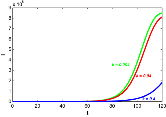
Trajectory profiles of symptomatically infected population (I) for different values of k

In Fig. 8, the impact of the growth of information and the ‘level for unresponsiveness towards information’ on the infected population have been observed. Here, p and q represent the ‘growth rate of information’ and the ‘level for unresponsiveness towards information’, respectively. Figure 8a depicts that increase in information can lower the infected population with time as people can successfully save themselves from getting infected by induced behavioural changes. On the other hand, decreasing the level of people unresponsiveness towards information (smaller value of q) ultimately decreases the symptomatically infected individuals with time (see Fig. 8b). It is known that increasing information reduce the infected population but if the response rate $(u_1)$ also starts to increase along with information, then the rate of decrease is higher. Figure 9 depicts that symptomatically infected population decrease significantly for increasing value of $u_1$ for increasing p.

Fig. 8.

Trajectory profiles of symptomatically infected population (I) for different values of a p and b q

Fig. 9.

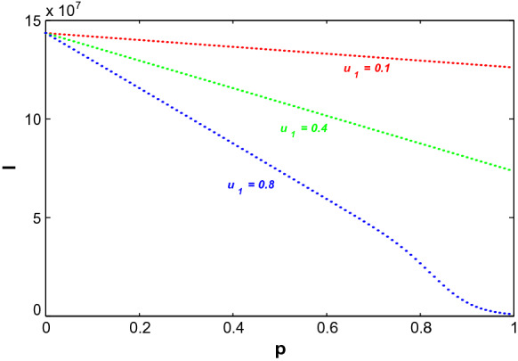
Variation of symptomatically infected population (I) due to change in growth of information, p for different values of $u_1$

Optimal control problem

We formulate the corresponding optimal control problem here to observe how suitable control interventions reduce the disease burden on the population. (a) The awareness programs among susceptible and symptomatically infected people regarding the information about COVID-19 and its symptoms so that the susceptible can take precautions and infected can admit to hospitals without neglecting the symptoms and (b) better treatment policies on hospitalised people have been considered as the control policies. We have analysed analytically and also numerically how these control policies make their impact on disease transmission and try to optimise the cost burden for their implementations.

(i) Increase the awareness among susceptible individuals and symptomatically infected individuals through information: Susceptible individuals start to become aware of a disease and its prevention when they are provided with enough information and this results in behavioural changes in population. The awareness programs to spread the information regarding COVID-19 outbreak has been considered as a possible tool to activate the sensibility of those individuals who live in a susceptible environment. These days Government and media sources have spread the news about this disease fatality regularly. And due to the regular broadcast, the people have started to take protective measures at a higher rate by maintaining social distances and proper hygiene, staying at isolation and even adopting the self-quarantine strategy. In system (1), $u_1$ represents the intensity of response through information with the restriction $0\le u_1\le 1.$ Here, 0 and 1, respectively, denotes no response and the full response of the informed population. As a consequence, $u_1(t)$ changes according to the individual’s behavioural response and we have taken this response intensity as one of the control variables. Incurred cost is involved as a nonlinear function of $u_1$ to stimulate the response of individuals and their behavioural changes. If the information starts to spread at a higher rate, then it may help to find the optimal response of susceptible individuals. Moreover, these awareness programs are conducted to aware not only the susceptible population but infected people too. It is a person’s responsibility to consult a medical person or to admit to a hospital if the slightest symptom is shown in his body. Anyone should not ignore by assuming it as a simple cough and cold case. By admitting to the hospital at an early stage can also decrease the disease burden and so, a saturated hospitalisation rate function ${\displaystyle \frac{{ϵ}_1{u}_{2}I}{1+{\zeta }_{1}I}}$ is incorporated in the system where ${ϵ}_1$ denotes the rate at which symptomatic infected individuals move to hospitals without ignoring the symptoms with intensity $u_2$ and saturation constant is ${\zeta }_1^{-1}$. The costs incurred in hospitalisation, medicines, etc., during the time a person admitted to a hospital or isolation centre is taken into consideration. The awareness intensity $u_2$ is taken as another control variable with restriction $0\le u_2\le 1$ where 1 denotes when a person admits into a hospital without ignoring the symptoms whenever feel sick. And 0 denotes the case when a person becomes ignorant about his sickness and does not consult a doctor.

(ii) Better treatment policy for hospitalised individual: Providing proper and better antidote of a virus to the hospitalised people at an early stage of infection can lower the disease fatality. It affects disease progression too. It is considered that the treatment which is available and provided to the individuals admitted in the hospitals is of limited quantity. The resource availabilities depend on medical diagnosis, financial stability, treatment, etc., and all these things are limited. Considering this fact, a saturated treatment rate function ${\displaystyle \frac{{ϵ}_2{u}_{3}H}{1+{\zeta }_{2}H}}$ is incorporated in the system where ${ϵ}_2$ denotes treatment rate with intensity $u_3$ and saturation constant is ${\zeta }_2^{-1}$. The cost incurred in vaccination, medicines, diagnosis, health care, hospitalisation, etc., at the time of treatment period is taken into consideration. The treatment intensity $u_3$ is taken as another control variable with restriction $0\le u_3\le 1$ where 0 and 1 denote the no response and full response to the given treatment, respectively.

The main work is to determine optimal response intensity and optimal treatment with minimum cost by the help of provided information. So, the region for the control interventions $u_1(t),u_2(t)$ and $u_3(t)$ is given as:

$$\begin{array}{cc}\hfill \mathrm{\Pi }=& \left\{\left(u_1,(t),,,u_2,(t),,,u_3,(t)\right),|,\left(u_1,(t),,,u_2,(t),,,u_3,(t)\right)\right)\hfill \\ \hfill & \left(\in ,[0,1],\times ,[0,1],\times ,[0,1],,,t,\in ,[0,T_f]\right\},\hfill \end{array}$$

where $T_f$ is the final time up to which the control policies are executed, and also $u_i(t)$ for $i=1,2,3$ are measurable and bounded functions.

Determination of total cost

We determine the incurred cost which needs to be minimised in order to apply control interventions.

(i) Cost involved to spread awareness among susceptible and symptomatic infected people: The total cost incurred during awareness spreading programs among people is given as:

$$\begin{array}{c}\hfill {\int }_0^{T_f}\left[w_1,I,(t),+,w_3,u_1^2,(t),+,w_4,u_2^2,(t)\right]\mathrm{d}t\end{array}$$

The cost for spreading awareness among susceptible regarding the disease, necessary precautions and prevention by maintaining social distance and hygiene via social campaigns, newspapers, television, social networks, etc., is denoted by $w_3{u}_1^2(t)$. The term considers the cost of associated efforts to realise the individual about the importance of maintaining social distances and it is observed that this cost is high enough. Moreover, the cost incurred when symptomatically infected individual consults a medical person and admits to a hospital without ignoring the symptoms is represented by the term $w_{1}I(t)+w_4{u}_2^2(t)$. This cost includes the expenditure of hospitalisation, medicines, etc., and $w_4{u}_2^2(t)$ considers the productivity loss due to illness. There are some studies already exist which reveal the impact of the cost associated with awareness programs, screening and self-protective measures and nonlinearity up to order two have been taken [2, 4, 25]. We, in this work, now emphasise on the fact how the awareness programs and practical cautions reduce the disease burden at the time of this epidemic outbreak.

(ii) Cost involved during treatment at hospitals: Total cost associated with treatment for symptomatic infected individual is given as:

$$\begin{array}{c}\hfill {\int }_0^{T_f}\left[w_2,H,(t),+,w_5,u_3^2,(t)\right]\mathrm{d}t,\end{array}$$

where $w_{2}H(t)$ and $w_5{u}_3^2(t)$, respectively, denote the cost associated with hospitalised population for losing man power [17, 23, 25] and the cost at the time of treatment due to diagnosis charges, the expenditure of hospitalisation, etc. The later term considers the opportunity loss including productivity loss due to admittance to the hospital. So, the nonlinearity of $u_3(t)$ is taken up to order two for treatment policy [17, 23, 25].

The following control problem is considered based on previous discussions along with the cost functional J to be minimised:

$$\begin{array}{cc}& J[u_1(t),u_2(t),u_3(t)]\hfill \\ \hfill & ={\int }_0^{T_f}\left[w_1,I,(t),+,w_2,H,(t),+,w_3,u_1^2,(t)\right)\hfill \\ \hfill & \left(+,w_4,u_2^2,(t),+,w_5,u_3^2,(t)\right]\mathrm{d}t\hfill \end{array}$$ 5

subject to the model system:

$$\begin{array}{cc}\hfill \frac{\text{d}S}{\text{d}t}=& \mathrm{\Lambda }-({\beta }_{1}A+{\beta }_{2}I+{\beta }_{3}H)S-dS\hfill \\ \hfill & +\xi R-u_1(t)kSZ,\hfill \\ \hfill \frac{\text{d}E}{\text{d}t}=& ({\beta }_{1}A+{\beta }_{2}I+{\beta }_{3}H)S-(\kappa +d)E,\hfill \\ \hfill \frac{\text{d}A}{\text{d}t}=& \kappa \varphi E-\eta A-(d+{\delta }_1)A,\hfill \\ \hfill \frac{\text{d}I}{\text{d}t}=& \kappa (1-\varphi )E+\eta A-(\omega +d+{\delta }_2)I\hfill \\ \hfill & -\frac{{ϵ}_1{u}_2(t)I}{1+{\zeta }_{1}I},\hfill \\ \hfill \frac{\text{d}H}{\text{d}t}=& \omega I-\gamma H-(d+{\delta }_3)H+\frac{{ϵ}_1{u}_2(t)I}{1+{\zeta }_{1}I}\hfill \\ \hfill & -\frac{{ϵ}_2{u}_3(t)H}{1+{\zeta }_{2}H},\hfill \\ \hfill \frac{\text{d}R}{\text{d}t}=& \gamma H-dR-\xi R+u_1(t)kSZ\hfill \\ \hfill & +\frac{{ϵ}_2{u}_3(t)H}{1+{\zeta }_{2}H},\hfill \\ \hfill \frac{\text{d}Z}{\text{d}t}=& \frac{\mathit{pI}}{1+qI}-a_{0}Z,\hfill \end{array}$$ 6

with initial conditions $S(0)>0,E(0)\ge 0,A(0)\ge 0,I(0)\ge 0,H(0)\ge 0,R(0)\ge 0$ and $Z(0)\ge 0.$ Here, the functional J denotes the total incurred cost as stated and the integrand:

$$\begin{array}{cc}& L(S,E,A,I,H,R,Z,u_1(t),u_2(t),u_3(t))\hfill \\ \hfill & =w_{1}I(t)+w_{2}H(t)+w_3{u}_1^2(t)\hfill \\ \hfill & +w_4{u}_2^2(t)+w_5{u}_3^2(t)\hfill \end{array}$$

denotes the cost at time t. Positive parameters $w_1,w_2,w_3,w_4\text{and}{w}_5$ are weight constants balancing the units of the integrand [17, 25]. The optimal control interventions $u_1^{\ast },u_2^{\ast }$ and $u_3^{\ast }$, exist in $\mathrm{\Pi }$, mainly minimise the cost functional J.

Theorem 9.1

The optimal control interventions $u_1^{\ast },u_2^{\ast }$ and $u_3^{\ast }$ in $\mathrm{\Pi }$ of the control system (5)–(6) exist such that $J(u_1^{\ast },u_2^{\ast },u_3^{\ast })=min[J(u_1,u_2,u_3)]$.

Proof

Proof is done in “Appendix”. $\square$

Pontryagin’s Maximum Principle helps to obtain optimal controls $u_1^{\ast },u_2^{\ast }$ and $u_3^{\ast }$ of system (5)–(6).

Theorem 9.2

If $u_1^{\ast },u_2^{\ast }$ and $u_3^{\ast }$ are the optimal control variables and $S^{\ast },E^{\ast },A^{\ast },I^{\ast },H^{\ast },R^{\ast },Z^{\ast }$ are corresponding optimal state variables of the control system (5)–(6), then there exist adjoint variables $\lambda =\left({\lambda }_1,,,{\lambda }_2,,,\dots ,,,{\lambda }_7\right)\in {\mathbb{R}}^7$ satisfying the canonical equations:

$$\begin{array}{c}\hfill \begin{array}{cc}\hfill \frac{\mathrm{d}{\lambda }_1}{\mathrm{d}t}& ={\lambda }_1[{\beta }_{1}A+{\beta }_{2}I+{\beta }_{3}H+d+u_{1}kZ]\hfill \\ \hfill & -{\lambda }_2({\beta }_{1}A+{\beta }_{2}I+{\beta }_{3}H)-{\lambda }_6(u_{1}kZ)\hfill \\ \hfill \frac{\mathrm{d}{\lambda }_2}{\mathrm{d}t}& ={\lambda }_2(d+\kappa )-{\lambda }_3(\kappa \varphi )-{\lambda }_4\{\kappa (1-\varphi )\}\hfill \\ \hfill \frac{\mathrm{d}{\lambda }_3}{\mathrm{d}t}& ={\lambda }_1({\beta }_{1}S)-{\lambda }_2({\beta }_{1}S)\hfill \\ \hfill & +{\lambda }_3(\eta +d+{\delta }_1)-{\lambda }_4(\eta )\hfill \\ \hfill \frac{\mathrm{d}{\lambda }_4}{\mathrm{d}t}& =-w_1+{\lambda }_1({\beta }_{2}S)-{\lambda }_2({\beta }_{2}S)\hfill \\ \hfill & +{\lambda }_4\left\{\omega ,+,d,+,{\delta }_2,+,\frac{{ϵ}_1{u}_2}{{(1+{\zeta }_{1}I)}^2}\right\}\hfill \\ \hfill & -{\lambda }_5\left\{\omega ,+,\frac{{ϵ}_1{u}_2}{{(1+{\zeta }_{1}I)}^2}\right\}\hfill \\ \hfill & -{\lambda }_7\left\{\frac{p}{{(1+qI)}^2}\right\}\hfill \\ \hfill \frac{\mathrm{d}{\lambda }_5}{\mathrm{d}t}& =-w_2+{\lambda }_1({\beta }_{3}S)-{\lambda }_2({\beta }_{3}S)\hfill \\ \hfill & +{\lambda }_5\left\{\gamma ,+,d,+,{\delta }_3,+,\frac{{ϵ}_2{u}_3}{{(1+{\zeta }_{2}H)}^2}\right\}\hfill \\ \hfill & -{\lambda }_6\left\{\gamma ,+,\frac{{ϵ}_2{u}_3}{{(1+{\zeta }_{2}H)}^2}\right\}\hfill \\ \hfill \frac{\mathrm{d}{\lambda }_6}{\mathrm{d}t}& =-{\lambda }_1(\xi )+{\lambda }_6(d+\xi )\hfill \\ \hfill \frac{\mathrm{d}{\lambda }_7}{\mathrm{d}t}& ={\lambda }_1(u_{1}kS)-{\lambda }_6(u_{1}kS)+{\lambda }_7(a_0)\hfill \end{array}\end{array}$$ 7

with transversality conditions ${\lambda }_i(T_f)=0$ for $i=1,2,\dots ,7$ and corresponding optimal controls $u_1^{\ast },u_2^{\ast }$ and $u_3^{\ast }$ are given as:

$$\begin{array}{c}\hfill \begin{array}{cc}\hfill u_1^{\ast }& =min\left\{max,\left\{0,,,\left(\frac{k{S}^{\ast }{Z}^{\ast }}{2w_3},\left({\lambda }_1,-,{\lambda }_6\right)\right)\right\},,,1\right\},\hfill \\ \hfill u_2^{\ast }& =min\left\{max,\left\{0,,,\left(\frac{{ϵ}_1{I}^{\ast }}{2w_4\left(1,+,{\zeta }_1,I^{\ast }\right)},\left({\lambda }_4,-,{\lambda }_5\right)\right)\right\},,,1\right\},\hfill \\ \hfill and{u}_3^{\ast }& =min\left\{max,\left\{0,,,\left(\frac{{ϵ}_2{H}^{\ast }}{2w_5\left(1,+,{\zeta }_2,H^{\ast }\right)},\left({\lambda }_5,-,{\lambda }_6\right)\right)\right\},,,1\right\}.\hfill \end{array}\\ \hfill \end{array}$$ 8

Proof

Proof is given in “Appendix”. $\square$

Numerical results with control policies

In system (6), different control strategies have been applied to reduce the disease burden and to minimise the total cost by finding the optimal control paths. The growth of information varies with time as it depends on disease fatality and behavioural response. So, $u_1$ is taken as a control variable. Also, there exist two other control variables $u_2$ and $u_3$ representing hospitalisation of symptomatically infected without neglecting symptoms and better treatment of hospitalised people, respectively. The positive weights are taken as $w_1=1,w_2=1,w_3=2500,w_4=10$ and $w_5=100$ [17, 25]. In order to draw the numerical figures, we slightly adjust ${\beta }_i$ for $i=1,2,3$ and $\varphi$ and all the parameters are listed in Table 2. The effects of implementation of one or all control strategies to find the minimal cost have been analysed one by one here. Corresponding control system in Eqs. (5)–(6) is solved here with the initial population size: $S(0)=135\times {10}^4,E(0)=500,A(0)=10,I(0)=40,H(0)=15,R(0)=5$ and $Z(0)=1$. Four different cases are considered: (i) when only $u_1$ is applied, (ii) when $u_1$ and $u_2$ are applied, (iii) when $u_1$ and $u_3$ are applied and (iv) when all control policies are applied. The numerical simulation for all cases is obtained by MATLAB. The optimal control variables are found by Forward-backward sweep method where the optimal state system and the adjoint state system are solved by forward and backward in time, respectively. In the next step, the steepest descent method is used to update the optimal controls by Hamiltonian for the optimality of the system [26] and the process continues until the convergence. It is assumed that the control policies are applied for approximately $T_f=90$ days. In India, the first case of COVID-19 was registered on 30 January 2020 and still now the number of affected cases are increasing day by day. The first lockdown is announced in March and observing the severity, the Government has extended its duration. The people are strictly advised to maintain social distancing and proper hygiene in order to keep themselves safe. As there is no vaccine discovered still now, so, natural immunity and physical distancing are the only way-outs to avoid from being infected. We have taken (i) awareness among susceptible individuals $(u_1)$, (ii) awareness among infected individuals $(u_2)$ and (iii) better treatment $(u_3)$ as our control policies and looking at the current situation, it is observed that people need to maintain these precautions for quite a long time.

Table 2.

Parametric values used in model system (6)

Parametric values
$\mathrm{\Lambda }$	$7\times {10}^4$	${\beta }_1$	$0.5\times {10}^{-10}$
${\beta }_2$	$2\times {10}^{-9}$	${\beta }_3$	$1.2\times {10}^{-10}$
$\xi$	$3\times {10}^{-10}$	$u_1$	0.1
k	0.002	$\kappa$	0.6
$\varphi$	0.3	$\eta$	0.15
${\delta }_1$	${10}^{-4}$	${\delta }_2$	$5\times {10}^{-4}$
${\delta }_3$	$8\times {10}^{-4}$	$\omega$	0.02
$\gamma$	0.5	d	0.000055
p	0.01	q	1
$a_0$	0.06	${ϵ}_1$	0.1
${ϵ}_2$	0.9	${\zeta }_1$	0.05
${\zeta }_2$	0.01	$w_1$	1
$w_2$	1	$w_3$	2500
$w_4$	10	$w_5$	100

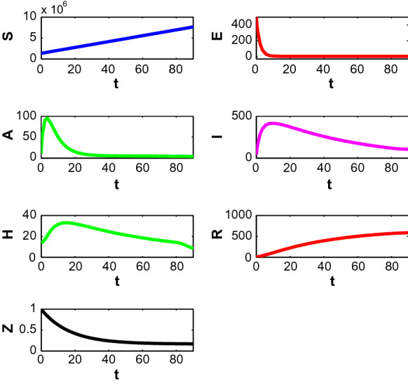
First, we consider the case when people only adopt behavioural changes in a susceptible environment. Figure 10 depicts the population profiles when $u_1=u_1^{\ast }$ and $u_2=u_3=0$. At $T_f=90$, the population become (7,647,536.63, 6.2058, 6.0621, 203.3930, 13.79, 561.30, 0.169704). The susceptible population increases with time. Both asymptomatically and symptomatically infected population increase steeply within 7–10 days and reach their maximum values but after that, the slope of the trajectories start to decrease. It is noted that the rate of declination is higher for asymptomatically infected people. Also, the number of asymptomatically infected people is lower than the number of symptomatically infected people. Hospitalised people also decreases with time almost after the first 2 weeks as recovered people increases. The corresponding optimal control path is given in Fig. 11. The intensity of the control variable works with higher intensity at earlier days but later it decreases with time. The declination of the graph may be caused because of people ignorance, etc.

Fig. 10.

Profiles of populations with applied optimal control $u_1^{\ast }$ only and $u_2=u_3=0$

Fig. 11.

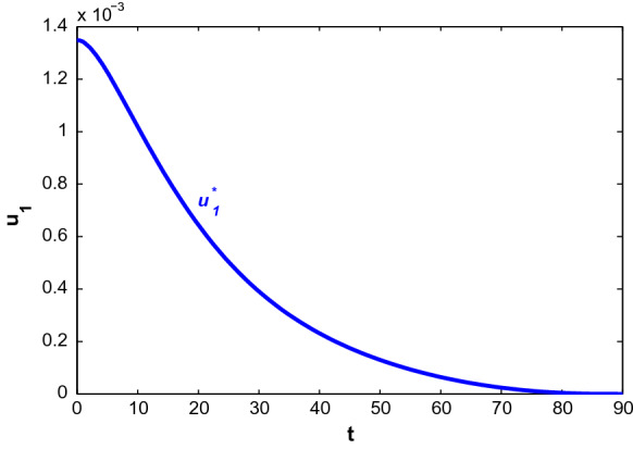
Profiles of populations with applied optimal control $u_1^{\ast }$ only and $u_2=u_3=0$

Next, we consider the case when susceptible people take precautions to avoid being infected $(u_1)$ and also symptomatically infected individuals enter into hospitals even when they are shown slightest symptoms $(u_2)$. Figure 12 shows the population trajectories when $u_1=u_1^{\ast }$ and $u_2=u_2^{\ast }$ but $u_3=0$. At $T_f=90$, the population becomes (7,647,620.98, 3.2498, 3.3487, 106.0726, 8.60, 587.64, 0.169182). It is observed that the number of symptomatically infected people decreases significantly in this case. Also, the recovered population increases here. Both the infected population first increase and then decrease after almost 1 week. Figure 13 shows the optimal control paths of $u_1$ and $u_2$. From this figure, it is observed that $u_1$ works with lesser intensity than $u_2$. Moreover, the intensity of $u_1$ gradually decreases with time. But $u_2$ works with its maximum intensity for quite a long time and then decreases suddenly.

Fig. 12.

Profiles of populations with applied optimal controls $u_1^{\ast }$ and $u_2^{\ast }$ only and $u_3=0$

Fig. 13.

Optimal controls $u_1^{\ast }$ and $u_2^{\ast }$ when $u_3=0$

Now we consider the case when people induce behavioural changes to protect themselves in susceptible stage $(u_1)$ and also hospitalised people are provided with better treatment $(u_3)$. Figure 14 depicts the population profiles for $u_1=u_1^{\ast }$ and $u_3=u_3^{\ast }$ but $u_2=0$. At $T_f=90$, the population becomes (7,647,547.32, 6.1961, 6.0521, 203.2271, 11.7627, 553.23, 0.169703). Implementation of $u_3$ increases susceptible population as more people are recovered in this case and so moved to susceptible class further. Corresponding optimal control paths are depicted in Fig. 15. The intensity of the control variable representing behavioural response decreases continuously with time and the intensity itself is not much higher. On the other hand, the intensity of $u_3$ first increases for almost 3 weeks and then decreases with a slower rate for next 2 months and then suddenly decreases. It represents that the treatment works with higher intensity at the earlier state and with time the intensity decreases when people become aware of the disease and its precautions.

Fig. 14.

Profiles of populations with applied optimal controls $u_1^{\ast }$ and $u_3^{\ast }$ only and $u_2=0$

Fig. 15.

Optimal controls $u_1^{\ast }$ and $u_3^{\ast }$ when $u_2=0$

It is obvious that implementing all the control policies is beneficial for the proposed system. So, we consider the combination of all three control policies in the system, i.e. a system where people induce behavioural changes with time to protect themselves from infection, symptomatically infected people move to a hospital without neglecting symptoms and better treatment is applied to hospitalised people. Figure 16 depicts the population trajectories in the presence of all control policies. At $T_f=90$, population becomes (7,647,630.40, 3.2391, 3.3381, 105.8244, 7.2543, 580.2986, 0.169180). The susceptible population increases at the highest level in this case. Also, both the infected population decreases at its lowest population here. Moreover, the recovered population is higher than the case when only $u_1$ is applied. Figure 17 shows the paths of optimal control strategies. The control policy on behavioural response works with higher intensity for few days but after that, it starts to decrease. It is justifiable as people become curious when epidemic or pandemic first outbreaks and they try to adopt changes in behaviour based on the information received but later it turns into their usual habit. Moreover, the infected people, if take the slightest symptoms seriously and consult medical person immediately, then it can reduce the disease also. Again, if the hospitalised people are provided with a proper antidote and better treatment, it helps to increase the number of recovered people. Here, $u_2$ acts with maximum intensity for a long time and then it decreases. $u_3$ also acts with its higher intensity for almost one and a half month following a declination at a very slow rate.

Fig. 16.

Profiles of populations with both optimal control policies $u_1^{\ast },u_2^{\ast }$ and $u_3^{\ast }$

Fig. 17.

Profiles of optimal controls $u_1^{\ast },u_2^{\ast }$ and $u_3^{\ast }$

In Fig. 18, cost design analysis has been performed in the absence and presence of $u_2$ and $u_3$ but we have considered $u_1$ in both the cases. There is one case where all three control policies are applied and the next case is when only the behavioural response is considered. Optimal cost profiles are shown in Fig. 18a for the cases and trajectory profiles for symptomatically infected individuals are depicted in Fig. 18b. In the absence of $u_2$ and $u_3$, cost occurs due to productivity loss by infected only. So, the opportunity loss is higher due to an epidemic outbreak and overall infected population increases in this case. On the other hand, the optimal cost is lower when all control interventions are applied. And as the infected population is lower in this case, it reduces the cost incurred because of opportunity loss.

Fig. 18.

a Cost distribution in presence and absence of control policies. b Profiles of symptomatic infected population under different control policies

Effect of hospitalisation rate and saturation constant on optimal control policies

If more symptomatically infected individuals admit into a hospital, then we observe how the hospitalisation rate and saturation constant have effects on the disease dynamics in the presence of the control policies with optimal intensities. Saturation rate $({\zeta }_1^{-1})$ and the hospitalisation rate $({ϵ}_1)$ have been varied in the following figures. Figure 19 shows the graphs of symptomatic infective population (I) and corresponding cost for different values of ${\zeta }_1$. For smaller saturation rate (larger values of ${\zeta }_1$), infective individuals and associated cost increase due to increase in productivity loss. Corresponding optimal control paths are drawn in Fig. 20 from which it is observed that for increasing value of ${\zeta }_1$, the control policy denoting behavioural response in susceptible individuals acts with a higher intensity which means smaller saturation rate increases the time period during which the control policy is implemented with higher intensity successfully. On the other hand, decreasing value of ${\zeta }_1$ increases the intensity level of the other two control interventions. Thus, if the saturation constant is high enough, then it is economically viable and hence, requires comparatively lesser efforts while implementing the control policies.

Fig. 19.

a Profiles of symptomatic infective population for various ${\zeta }_1$ with $u_1^{\ast },u_2^{\ast }$ and $u_3^{\ast }$. b Profiles of cost for various ${\zeta }_1$ with $u_1^{\ast },u_2^{\ast }$ and $u_3^{\ast }$

Fig. 20.

a Plots of control $u_1^{\ast }$ for various ${\zeta }_1$. b Plots of control $u_2^{\ast }$ for various ${\zeta }_1$. c Plots of control $u_3^{\ast }$ for various ${\zeta }_1$

Further with the increase in treatment rate $({ϵ}_1)$ from 0.01 to 0.1, the both symptomatic infective population and associated cost decrease with time (Fig. 21). From Fig. 22, it is observed that for increasing value of ${ϵ}_1$, the control policy denoting behavioural response in susceptible people works for a smaller time period. Also, increasing value of ${ϵ}_1$ increases the intensity level of the other two control variables. In Fig. 22b, c it is observed that the higher hospitalisation rate increases the lengths of maximum intensities of these two optimal control implementation periods. It means lesser efforts on these two applied controls are sufficient to reduce the overall infective population.

Fig. 21.

a Profiles of infective population for various ${ϵ}_1$ with $u_1^{\ast },u_2^{\ast }$ and $u_3^{\ast }$. b Profiles of cost for various ${ϵ}_1$ with $u_1^{\ast },u_2^{\ast }$ and $u_3^{\ast }$

Fig. 22.

a Plots of control $u_1^{\ast }$ for various ${ϵ}_1$. b Plots of control $u_2^{\ast }$ for various ${ϵ}_1$. c Plots of control $u_3^{\ast }$ for various ${ϵ}_1$

Conclusion

Coronavirus or Covid-19 first appeared in China in December 2019, but today it has spread all over the world in the form of a pandemic. Reports of the current situation reveal that almost 30 lakhs people are infected with the virus worldwide. Though the Governments and medical persons of each and every country are trying to provide protective measures to people, the infection rate is still high enough as the proper antidote for this virus is still unknown. According to the data till 26th April 2020, provided by the dashboard of CSSE at John Hopkins University, US has the highest confirmed cases with the number 939, 249 [6]. Though according to the official reports, almost 26, 384 people have died in Italy which is the highest in number among 185 countries or religions. If we consider the current situation in India, then from the reports of NIC, India, there are 20, 177 confirmed cases, 826 death cases and 5, 914 recovered cases are reported till 26th April [29]. Keeping this pandemic situation in mind, in this work, we have formulated a compartmental SEIRS model of Covid-19 where a separate equation is incorporated to reflect the information which induces behavioural changes. The growth rate of information is based on symptomatically infected individuals, awareness programs, social activities, etc. Positivity and boundedness of system variables guarantees that the proposed system is well-defined. Feasibility conditions of equilibrium points show that DFE exists for all parametric values where the unique endemic equilibrium point exists only when basic reproduction number $R_0$ exceeds unity. Both local and global stability conditions have been derived in Sect. 6. As we have only one endemic equilibrium point for $R_0>1$ and there does not exist any endemic point for $R_0<1$, hence, it is concluded that the system undergoes a forward (transcritical) bifurcation around the disease-free equilibrium. If the people start to take the information regarding the virus seriously and take its precautions, then it is obvious that overall infected population is lesser and it is shown in Fig. 7. Moreover, increasing values of the growth of information and decreasing ‘level for unresponsiveness towards information’ also help to reduce the infected population. Also, symptomatically infected population with respect to the growth rate of information decreases for increasing value of $u_1$, i.e. if people respond to the growing information regarding the awareness at a higher rate, then infected population decreases significantly. As the behavioural changes include keeping social distances, maintaining proper hygiene, staying at isolation and adopting the self-quarantine method, so, these precautions can really be useful to prevent the disease transmission at a higher rate.

In the later part, a corresponding optimal control problem is considered. Implementation of control interventions helps to reduce the disease burden. The behavioural changes in susceptible population changes with time and so, it is considered as one of the control policy. Further, the symptomatically infected people can also become cautious by the current disease fatality and may consult doctors or admit to hospitals if slightest symptoms are shown. Again, during the treatment period, better and proper medicines or diagnosis can be provided to a hospitalised person. So, all these things can be considered as control strategies. Numerical figures show that the control presenting behavioural response $(u_1)$ works with higher intensity immediately after implementation but gradually it decreases with time. On the other hand, the control policy denoting hospitalisation of infected individuals $(u_2)$ works with its maximum intensity for quite a long time period and then it decreases. Again, the control presenting better treatment of hospitalised people works with higher intensity for almost 2 months following a declination at a later stage, though this intensity is lower than the intensity of $u_2$. Implementation of a single strategy is useful but all the three control policies together can reduce the infected population and increase the recovered population at a higher rate. Hence, applying all the control policies together may help to reduce disease transmission at this current epidemic situation.

Appendix

Local stability of the endemic equilibrium point

Proof of Theorem 6.3

The Jacobian matrix at endemic equilibrium point $E^{\ast }$ is given as

$$\begin{array}{c}\hfill \overline{J}=\left(\begin{array}{ccccccc}{a}_{11}& 0& a_{13}& a_{14}& a_{15}& a_{16}& a_{17}\\ a_{21}& a_{22}& a_{23}& a_{24}& a_{25}& 0& 0\\ 0& a_{32}& a_{33}& 0& 0& 0& 0\\ 0& a_{42}& a_{43}& a_{44}& 0& 0& 0\\ 0& 0& 0& a_{54}& a_{55}& 0& 0\\ a_{61}& 0& 0& 0& a_{65}& a_{66}& a_{67}\\ 0& 0& 0& a_{74}& 0& 0& a_{77}\end{array}\right)\end{array}$$

where $a_{11}=-({\beta }_1{A}^{\ast }+{\beta }_2{I}^{\ast }+{\beta }_3{H}^{\ast })-d-u_{1}k{Z}^{\ast },a_{13}=-{\beta }_1{S}^{\ast },a_{14}=-{\beta }_2{S}^{\ast },a_{15}=-{\beta }_3{S}^{\ast },a_{16}=\xi ,a_{17}=u_{1}k{S}^{\ast },a_{21}={\beta }_1{A}^{\ast }+{\beta }_2{I}^{\ast }+{\beta }_3{H}^{\ast },a_{22}=-{\alpha }_0,a_{23}={\beta }_1{S}^{\ast },a_{24}={\beta }_2{S}^{\ast },a_{25}={\beta }_3{S}^{\ast },a_{32}=\kappa \varphi ,a_{33}=-{\alpha }_1,a_{42}=\kappa (1-\varphi ),a_{43}=\eta ,a_{44}=-{\alpha }_2,a_{54}=\omega ,a_{55}=-{\alpha }_3,a_{61}=u_{1}k{Z}^{\ast },a_{65}=\gamma ,a_{66}=-(d+\xi ),a_{67}=u_{1}k{S}^{\ast },a_{74}=\frac{p}{{(1+q{I}^{\ast })}^2}$ and $a_{77}=-a_0$.

Characteristic equation of $\overline{J}{|}_{E^{\ast }}$ is ${\lambda }^7+R_1{\lambda }^6+R_2{\lambda }^5+R_3{\lambda }^4+R_4{\lambda }^3+R_5{\lambda }^2+R_6\lambda +R_7=0,$

$$\begin{array}{cc}\hfill R_1& =-(a_{11}+a_{22}+a_{33}+a_{44}+a_{55}+a_{66}+a_{77}),\hfill \\ \hfill R_2& =a_{11}(a_{22}+a_{33}+a_{44}+a_{55}+a_{66}+a_{77})\hfill \\ \hfill & +a_{22}(a_{33}+a_{44}+a_{55}+a_{66}+a_{77})\hfill \\ \hfill & +a_{33}(a_{44}+a_{55}+a_{66}+a_{77})\hfill \\ \hfill & +a_{44}(a_{55}+a_{66}+a_{77})+a_{55}(a_{66}+a_{77})+a_{66}{a}_{77}\hfill \\ \hfill & -a_{16}{a}_{61}-a_{23}{a}_{32}-a_{24}{a}_{42}\hfill \\ \hfill R_3& =-[a_{11}{a}_{22}(a_{33}+a_{44}+a_{55}+a_{66}+a_{77})\hfill \\ \hfill & -a_{11}{a}_{23}{a}_{32}-a_{11}{a}_{24}{a}_{42}+a_{11}{a}_{55}(a_{66}+a_{77})\hfill \\ \hfill & +a_{11}{a}_{33}(a_{44}+a_{55}+a_{66}+a_{77})\hfill \\ \hfill & +a_{11}{a}_{44}(a_{55}+a_{66}+a_{77})\hfill \\ \hfill & +a_{11}{a}_{66}{a}_{77}+a_{13}{a}_{21}{a}_{32}+a_{14}{a}_{42}{a}_{21}\hfill \\ \hfill & -a_{16}{a}_{61}(a_{22}+a_{33}+a_{44}+a_{55}+a_{77})\hfill \\ \hfill & +a_{22}{a}_{33}(a_{44}+a_{55}+a_{66}+a_{77})\hfill \\ \hfill & +a_{22}{a}_{44}(a_{55}+a_{66}+a_{77})\hfill \\ \hfill & +a_{22}{a}_{55}(a_{66}+a_{77})+a_{22}{a}_{66}{a}_{77}\hfill \\ \hfill & -a_{23}{a}_{32}(a_{44}+a_{55}+a_{66}+a_{77})+a_{43}{a}_{32}{a}_{24}\hfill \\ \hfill & -a_{24}{a}_{42}(a_{33}+a_{55}+a_{66}+a_{77})+a_{54}{a}_{42}{a}_{25}\hfill \\ \hfill & +a_{33}{a}_{44}(a_{55}+a_{66}+a_{77})+a_{33}{a}_{55}(a_{66}+a_{77})\hfill \\ \hfill & +a_{33}{a}_{66}{a}_{77}+a_{44}{a}_{55}(a_{66}+a_{77})\hfill \\ \hfill & +a_{66}{a}_{77}(a_{44}+a_{55})]\hfill \end{array}$$

$$\begin{array}{cc}\hfill R_4& =-[-a_{11}{a}_{22}{a}_{33}(a_{44}+a_{55}+a_{66}+a_{77})\hfill \\ \hfill & -a_{11}{a}_{22}{a}_{44}(a_{55}+a_{66}+a_{77})\hfill \\ \hfill & -a_{11}{a}_{22}{a}_{55}(a_{66}+a_{77})-a_{11}{a}_{22}{a}_{66}{a}_{77}\hfill \\ \hfill & +a_{11}{a}_{23}{a}_{32}(a_{44}+a_{55}+a_{66}+a_{77})\hfill \\ \hfill & -a_{11}{a}_{24}{a}_{32}{a}_{43}+a_{11}{a}_{24}{a}_{42}\hfill \\ \hfill & (a_{33}+a_{55}+a_{66}+a_{77})-a_{11}{a}_{25}{a}_{42}{a}_{54}\hfill \\ \hfill & -a_{11}{a}_{33}{a}_{44}(a_{55}+a_{66}+a_{77})\hfill \\ \hfill & -a_{11}{a}_{33}{a}_{55}(a_{66}+a_{77})-a_{11}{a}_{33}{a}_{66}{a}_{77}\hfill \\ \hfill & -a_{11}{a}_{44}{a}_{55}(a_{66}+a_{77})\hfill \\ \hfill & -a_{11}{a}_{66}{a}_{77}(a_{44}+a_{55})\hfill \\ \hfill & -a_{13}{a}_{32}{a}_{21}(a_{44}+a_{55}+a_{66}+a_{77})\hfill \\ \hfill & +a_{14}{a}_{43}{a}_{32}{a}_{21}\hfill \\ \hfill & -a_{14}{a}_{42}{a}_{21}(a_{33}+a_{55}+a_{66}+a_{77})\hfill \\ \hfill & +a_{15}{a}_{54}{a}_{42}{a}_{21}\hfill \\ \hfill & +a_{16}{a}_{22}{a}_{61}(a_{33}+a_{44}+a_{55}+a_{77})\hfill \\ \hfill & -a_{16}{a}_{61}(a_{23}{a}_{32}+a_{24}{a}_{42})\hfill \\ \hfill & +a_{16}{a}_{33}{a}_{61}(a_{44}+a_{55}+a_{77})\hfill \\ \hfill & +a_{16}{a}_{44}{a}_{61}(a_{55}+a_{77})\hfill \\ \hfill & +a_{16}{a}_{55}{a}_{61}{a}_{77}\hfill \\ \hfill & +a_{74}{a}_{42}{a}_{21}{a}_{17}\hfill \\ \hfill & -a_{22}{a}_{33}{a}_{44}(a_{55}+a_{66}+a_{77})\hfill \\ \hfill & -a_{22}{a}_{33}{a}_{55}(a_{66}+a_{77})-a_{22}{a}_{33}{a}_{66}{a}_{77}\hfill \\ \hfill & -a_{22}{a}_{44}{a}_{55}(a_{66}+a_{77})\hfill \\ \hfill & -a_{22}{a}_{66}{a}_{77}(a_{44}+a_{55})\hfill \\ \hfill & +a_{23}{a}_{32}{a}_{44}(a_{55}+a_{66}+a_{77})\hfill \\ \hfill & +a_{23}{a}_{32}{a}_{55}(a_{66}+a_{77})+a_{22}{a}_{32}{a}_{66}{a}_{77}\hfill \\ \hfill & -a_{24}{a}_{32}{a}_{43}(a_{55}+a_{66}+a_{77})\hfill \\ \hfill & +a_{24}{a}_{33}{a}_{42}(a_{55}+a_{66}+a_{77})\hfill \\ \hfill & +a_{24}{a}_{42}{a}_{55}(a_{66}+a_{77})+a_{24}{a}_{42}{a}_{66}{a}_{77}\hfill \\ \hfill & +a_{25}{a}_{32}{a}_{43}{a}_{54}-a_{24}{a}_{42}{a}_{54}(a_{33}+a_{66}+a_{77})\hfill \\ \hfill & -a_{33}{a}_{44}{a}_{55}(a_{66}+a_{77})-a_{33}{a}_{66}\hfill \\ \hfill & a_{77}(a_{44}+a_{55})-a_{44}{a}_{55}{a}_{66}{a}_{77}]\hfill \end{array}$$

$$\begin{array}{cc}\hfill R_5& =-[a_{11}{a}_{22}{a}_{33}{a}_{44}(a_{55}+a_{66}+a_{77})\hfill \\ \hfill & +a_{11}{a}_{22}{a}_{33}{a}_{55}(a_{66}+a_{77})\hfill \\ \hfill & +a_{11}{a}_{32}{a}_{33}{a}_{66}{a}_{77}\hfill \\ \hfill & +a_{11}{a}_{22}{a}_{44}{a}_{55}(a_{66}+a_{77})\hfill \\ \hfill & +a_{11}{a}_{22}{a}_{66}{a}_{77}(a_{44}+a_{55})\hfill \\ \hfill & -a_{11}{a}_{23}{a}_{32}{a}_{44}(a_{55}+a_{66}+a_{77})\hfill \\ \hfill & -a_{11}{a}_{23}{a}_{32}{a}_{55}(a_{66}+a_{77})-a_{11}{a}_{23}{a}_{32}{a}_{66}{a}_{77}\hfill \\ \hfill & +a_{11}{a}_{24}{a}_{32}{a}_{43}(a_{55}+a_{66}+a_{77})\hfill \\ \hfill & -a_{11}{a}_{24}{a}_{33}{a}_{42}(a_{55}+a_{66}+a_{77})\hfill \\ \hfill & -a_{11}{a}_{24}{a}_{42}{a}_{55}(a_{66}+a_{77})\hfill \\ \hfill & -a_{11}{a}_{24}{a}_{42}{a}_{66}{a}_{77}-a_{11}{a}_{25}{a}_{32}\hfill \\ \hfill & a_{43}{a}_{54}+a_{11}{a}_{25}{a}_{33}{a}_{42}{a}_{54}\hfill \\ \hfill & +a_{11}{a}_{25}{a}_{42}{a}_{54}(a_{66}+a_{77})\hfill \\ \hfill & +a_{11}{a}_{33}{a}_{44}{a}_{55}(a_{66}+a_{77})\hfill \\ \hfill & +a_{11}{a}_{33}{a}_{66}{a}_{77}(a_{44}+a_{55})\hfill \\ \hfill & +a_{11}{a}_{44}{a}_{55}{a}_{66}{a}_{77}\hfill \\ \hfill & +a_{13}{a}_{21}{a}_{32}{a}_{44}(a_{55}+a_{66}+a_{77})\hfill \\ \hfill & +a_{13}{a}_{21}{a}_{32}{a}_{55}(a_{66}+a_{77})\hfill \\ \hfill & +a_{13}{a}_{21}{a}_{32}{a}_{66}{a}_{77}\hfill \\ \hfill & -a_{14}{a}_{21}{a}_{32}{a}_{43}(a_{55}+a_{66}+a_{77})\hfill \\ \hfill & +a_{14}{a}_{21}{a}_{33}{a}_{42}(a_{55}+a_{66}+a_{77})\hfill \\ \hfill & +a_{44}{a}_{21}{a}_{42}{a}_{55}(a_{66}+a_{77})\hfill \\ \hfill & +a_{14}{a}_{21}{a}_{42}{a}_{66}{a}_{77}\hfill \\ \hfill & +a_{15}{a}_{21}{a}_{32}{a}_{43}{a}_{54}\hfill \\ \hfill & -a_{15}{a}_{21}{a}_{42}{a}_{54}(a_{33}+a_{66}+a_{77})\hfill \\ \hfill & +a_{65}{a}_{54}{a}_{42}{a}_{21}{a}_{16}+a_{16}{a}_{67}{a}_{74}{a}_{42}{a}_{21}\hfill \\ \hfill & -a_{16}{a}_{22}{a}_{33}{a}_{61}(a_{44}+a_{55}+a_{77})\hfill \\ \hfill & -a_{16}{a}_{22}{a}_{44}{a}_{61}(a_{55}+a_{77})\hfill \\ \hfill & -a_{16}{a}_{22}{a}_{55}{a}_{61}{a}_{77}\hfill \\ \hfill & +a_{16}{a}_{23}{a}_{32}{a}_{61}(a_{44}+a_{55}+a_{77})\hfill \\ \hfill & -a_{16}{a}_{24}{a}_{32}{a}_{43}{a}_{61}\hfill \\ \hfill & +a_{16}{a}_{24}{a}_{42}{a}_{61}(a_{33}+a_{55}+a_{77})\hfill \\ \hfill & -a_{16}{a}_{25}{a}_{42}{a}_{54}{a}_{61}\hfill \\ \hfill & -a_{16}{a}_{33}{a}_{44}{a}_{61}(a_{55}+a_{77})\hfill \\ \hfill & -a_{16}{a}_{33}{a}_{55}{a}_{61}{a}_{77}\hfill \\ \hfill & -a_{16}{a}_{44}{a}_{55}{a}_{61}{a}_{77}+a_{17}{a}_{21}{a}_{32}{a}_{43}{a}_{74}\hfill \\ \hfill & -a_{74}{a}_{42}{a}_{21}{a}_{17}(a_{33}{a}_{55}+a_{66})\hfill \\ \hfill & +a_{22}{a}_{33}{a}_{44}{a}_{55}(a_{66}+a_{77})\hfill \\ \hfill & +a_{22}{a}_{33}(a_{44}+a_{55})a_{66}{a}_{77}\hfill \\ \hfill & +a_{22}{a}_{44}{a}_{55}{a}_{66}{a}_{77}\hfill \\ \hfill & -a_{23}{a}_{32}{a}_{44}{a}_{55}(a_{66}+a_{77})\hfill \\ \hfill & -a_{23}{a}_{32}(a_{44}+a_{55})a_{66}{a}_{77}\hfill \\ \hfill & +a_{24}{a}_{32}{a}_{43}{a}_{55}(a_{66}+a_{77})\hfill \\ \hfill & +a_{24}{a}_{32}{a}_{43}{a}_{66}{a}_{77}\hfill \\ \hfill & -a_{24}{a}_{33}{a}_{42}{a}_{55}(a_{66}+a_{77})\hfill \\ \hfill & -a_{24}{a}_{42}{a}_{66}{a}_{77}(a_{33}+a_{55})\hfill \\ \hfill & -a_{25}{a}_{32}{a}_{43}{a}_{54}(a_{66}+a_{77})\hfill \\ \hfill & +a_{25}{a}_{33}{a}_{42}{a}_{54}(a_{66}+a_{77})\hfill \\ \hfill & +a_{25}{a}_{42}{a}_{54}{a}_{66}{a}_{77}+a_{33}{a}_{44}{a}_{55}{a}_{66}{a}_{77}]\hfill \end{array}$$

$$\begin{array}{cc}\hfill R_6& =-[-a_{11}{a}_{22}{a}_{33}{a}_{44}{a}_{55}(a_{66}+a_{77})\hfill \\ \hfill & -a_{11}{a}_{22}{a}_{33}(a_{44}+a_{55})a_{66}{a}_{77}\hfill \\ \hfill & -a_{11}{a}_{22}{a}_{44}{a}_{55}{a}_{66}{a}_{77}\hfill \\ \hfill & +a_{11}{a}_{23}{a}_{32}{a}_{44}{a}_{55}(a_{66}+a_{77})\hfill \\ \hfill & +a_{11}{a}_{23}{a}_{32}(a_{44}+a_{55})a_{66}\hfill \\ \hfill & -a_{11}{a}_{24}{a}_{32}{a}_{43}{a}_{55}(a_{66}+a_{77})\hfill \\ \hfill & -a_{11}{a}_{24}{a}_{32}{a}_{43}{a}_{66}{a}_{77}\hfill \\ \hfill & +a_{11}{a}_{24}{a}_{33}{a}_{42}{a}_{55}(a_{66}+a_{77})\hfill \\ \hfill & +a_{11}{a}_{24}{a}_{42}(a_{55}+a_{33})a_{66}{a}_{77}\hfill \\ \hfill & +a_{11}{a}_{25}{a}_{32}{a}_{43}{a}_{54}(a_{66}+a_{77})\hfill \\ \hfill & -a_{11}{a}_{25}{a}_{33}{a}_{42}{a}_{54}(a_{66}+a_{77})\hfill \\ \hfill & -a_{11}{a}_{25}{a}_{42}{a}_{54}{a}_{66}{a}_{77}\hfill \\ \hfill & -a_{11}{a}_{33}{a}_{44}{a}_{55}{a}_{66}{a}_{77}\hfill \\ \hfill & -a_{13}{a}_{21}{a}_{32}{a}_{44}{a}_{55}(a_{66}+a_{77})\hfill \\ \hfill & -a_{13}{a}_{21}{a}_{32}(a_{44}+a_{55})a_{66}{a}_{77}\hfill \\ \hfill & +a_{14}{a}_{21}{a}_{32}{a}_{43}{a}_{55}(a_{66}+a_{77})\hfill \\ \hfill & +a_{14}{a}_{21}{a}_{32}{a}_{43}{a}_{66}{a}_{77}\hfill \\ \hfill & -a_{14}{a}_{21}{a}_{33}{a}_{42}{a}_{55}(a_{66}+a_{77})\hfill \\ \hfill & -a_{14}{a}_{21}(a_{33}+a_{55})a_{42}{a}_{66}{a}_{77}\hfill \\ \hfill & -a_{15}{a}_{21}{a}_{32}{a}_{43}{a}_{54}(a_{66}+a_{77})\hfill \\ \hfill & +a_{15}{a}_{21}{a}_{33}{a}_{42}{a}_{54}(a_{66}+a_{77})\hfill \\ \hfill & +a_{15}{a}_{21}{a}_{42}{a}_{54}{a}_{66}{a}_{77}\hfill \\ \hfill & +a_{16}{a}_{21}{a}_{32}{a}_{43}(a_{54}{a}_{65}+a_{67}{a}_{74})\hfill \\ \hfill & -a_{16}{a}_{21}{a}_{33}{a}_{42}(a_{54}{a}_{65}+a_{67}{a}_{74})\hfill \\ \hfill & -a_{16}{a}_{21}{a}_{42}{a}_{54}{a}_{65}{a}_{77}\hfill \\ \hfill & -a_{16}{a}_{21}{a}_{42}{a}_{55}{a}_{67}{a}_{74}\hfill \\ \hfill & +a_{16}{a}_{22}{a}_{33}{a}_{44}{a}_{61}(a_{55}+a_{77})\hfill \\ \hfill & +a_{16}{a}_{22}{a}_{77}{a}_{55}{a}_{61}(a_{33}+a_{44})\hfill \\ \hfill & -a_{16}{a}_{23}{a}_{32}{a}_{44}{a}_{61}(a_{55}+a_{77})\hfill \\ \hfill & -a_{16}{a}_{23}{a}_{32}{a}_{55}{a}_{61}{a}_{77}\hfill \\ \hfill & +a_{16}{a}_{24}{a}_{32}{a}_{43}{a}_{61}(a_{55}+a_{77})\hfill \\ \hfill & -a_{16}{a}_{24}{a}_{33}{a}_{42}{a}_{61}(a_{55}+a_{77})\hfill \\ \hfill & +a_{16}{a}_{24}{a}_{42}{a}_{55}{a}_{61}{a}_{77}\hfill \\ \hfill & -a_{16}{a}_{25}{a}_{32}{a}_{43}{a}_{54}{a}_{61}\hfill \\ \hfill & +a_{16}{a}_{25}{a}_{42}{a}_{54}{a}_{61}(a_{33}+a_{77})\hfill \\ \hfill & +a_{16}{a}_{33}{a}_{44}{a}_{55}{a}_{61}{a}_{77}\hfill \\ \hfill & -a_{17}{a}_{21}{a}_{32}{a}_{43}{a}_{74}(a_{55}+a_{66})\hfill \\ \hfill & +a_{17}{a}_{21}{a}_{33}{a}_{42}{a}_{74}(a_{55}+a_{66})\hfill \\ \hfill & +a_{17}{a}_{21}{a}_{42}{a}_{55}{a}_{66}{a}_{74}\hfill \\ \hfill & -a_{22}{a}_{33}{a}_{44}{a}_{55}{a}_{66}{a}_{77}\hfill \\ \hfill & +a_{23}{a}_{32}{a}_{44}{a}_{55}{a}_{66}{a}_{77}\hfill \\ \hfill & -a_{24}{a}_{43}{a}_{55}{a}_{66}{a}_{77}\hfill \\ \hfill & +a_{24}{a}_{33}{a}_{42}{a}_{55}{a}_{66}{a}_{77}\hfill \\ \hfill & +a_{25}{a}_{32}{a}_{43}{a}_{54}{a}_{66}{a}_{77}\hfill \\ \hfill & -a_{25}{a}_{33}{a}_{42}{a}_{54}{a}_{66}{a}_{77}]\hfill \\ \hfill \end{array}$$

$$\begin{array}{cc}\hfill R_7& =a_{11}{a}_{23}{a}_{32}{a}_{44}{a}_{55}{a}_{66}{a}_{77}\hfill \\ \hfill & -a_{11}{a}_{24}{a}_{32}{a}_{43}{a}_{55}{a}_{66}{a}_{77}\hfill \\ \hfill & +a_{11}{a}_{24}{a}_{33}{a}_{42}{a}_{55}{a}_{66}{a}_{77}\hfill \\ \hfill & +a_{11}{a}_{25}{a}_{32}{a}_{43}{a}_{54}{a}_{66}{a}_{77}\hfill \\ \hfill & -a_{11}{a}_{25}{a}_{33}{a}_{42}{a}_{54}{a}_{66}{a}_{77}\hfill \\ \hfill & -a_{13}{a}_{21}{a}_{32}{a}_{44}{a}_{55}{a}_{66}{a}_{77}\hfill \\ \hfill & +a_{14}{a}_{21}{a}_{32}{a}_{43}{a}_{55}{a}_{66}{a}_{77}\hfill \\ \hfill & -a_{14}{a}_{21}{a}_{33}{a}_{42}{a}_{55}{a}_{66}{a}_{77}\hfill \\ \hfill & -a_{15}{a}_{21}{a}_{32}{a}_{43}{a}_{54}{a}_{66}{a}_{77}\hfill \\ \hfill & +a_{15}{a}_{21}{a}_{33}{a}_{42}{a}_{54}{a}_{66}{a}_{77}\hfill \\ \hfill & +a_{16}{a}_{21}{a}_{32}{a}_{43}{a}_{54}{a}_{65}{a}_{77}\hfill \\ \hfill & +a_{16}{a}_{21}{a}_{32}{a}_{43}{a}_{55}{a}_{67}{a}_{74}\hfill \\ \hfill & -a_{16}{a}_{21}{a}_{33}{a}_{42}{a}_{54}{a}_{65}{a}_{77}\hfill \\ \hfill & -a_{16}{a}_{21}{a}_{33}{a}_{42}{a}_{55}{a}_{67}{a}_{74}\hfill \\ \hfill & +a_{16}{a}_{22}{a}_{33}{a}_{44}{a}_{55}{a}_{61}{a}_{77}\hfill \\ \hfill & -a_{16}{a}_{23}{a}_{32}{a}_{44}{a}_{55}{a}_{61}{a}_{77}\hfill \\ \hfill & +a_{16}{a}_{24}(a_{32}{a}_{43}-a_{33}{a}_{42})a_{55}{a}_{61}{a}_{77}\hfill \\ \hfill & +a_{16}{a}_{25}(a_{33}{a}_{42}-a_{32}{a}_{43})a_{54}{a}_{61}{a}_{77}\hfill \\ \hfill & +a_{17}{a}_{21}(a_{33}{a}_{42}-a_{32}{a}_{43})a_{55}{a}_{66}{a}_{74}\hfill \\ \hfill & -a_{11}{a}_{22}{a}_{33}{a}_{44}{a}_{55}{a}_{66}{a}_{77}\hfill \end{array}$$

Let us consider

$$\begin{array}{c}\hfill \begin{array}{cc}\hfill {\mathrm{\Delta }}_1& =R_1,{\mathrm{\Delta }}_2=\left|\begin{array}{cc}{R}_1& 1\\ R_3& R_2\end{array}\right|,{\mathrm{\Delta }}_3=\left|\begin{array}{ccc}{R}_1& 1& 0\\ R_3& R_2& R_1\\ R_5& R_4& R_3\end{array}\right|,\hfill \\ \hfill {\mathrm{\Delta }}_4& =\left|\begin{array}{cccc}{R}_1& 1& 0& 0\\ R_3& R_2& R_1& 1\\ R_5& R_4& R_3& R_2\\ R_7& R_6& R_5& R_4\end{array}\right|,\hfill \\ \hfill {\mathrm{\Delta }}_5& =\left|\begin{array}{ccccc}{R}_1& 1& 0& 0& 0\\ R_3& R_2& R_1& 1& 0\\ R_5& R_4& R_3& R_2& R_1\\ R_7& R_6& R_5& R_4& R_3\\ 0& 0& R_7& R_6& R_5\end{array}\right|,\hfill \\ \hfill {\mathrm{\Delta }}_6& =\left|\begin{array}{cccccc}{R}_1& 1& 0& 0& 0& 0\\ R_3& R_2& R_1& 1& 0& 0\\ R_5& R_4& R_3& R_2& R_1& 1\\ R_7& R_6& R_5& R_4& R_3& R_2\\ 0& 0& R_7& R_6& R_5& R_4\\ 0& 0& 0& 0& R_7& R_6\end{array}\right|,\hfill \\ \hfill {\mathrm{\Delta }}_7& =Det(\overline{J}{|}_{E^{\ast }}).\hfill \end{array}\end{array}$$

By Routh–Hurwitz criterion, $E^{\ast }$ is locally asymptomatically stable (LAS) if and only if ${\mathrm{\Delta }}_i>0$ for $i=1,2,3,4,5,6,7$, i.e. equivalently

• (i)$R_i>0$ for $i=1,7;$
• (ii)${\mathrm{\Delta }}_i>0$ for $i=2,3,4,5,6$.

$\square$

Existence of optimal control functions

Now we derive the conditions for existence of optimal control interventions which also minimise the cost function J in a finite time period.

Proof of Theorem 9.1

The optimal control variables, when exist, satisfy the following conditions:

• (i)Solutions of system (6) with control variables $u_1,u_2$ and $u_3$ in $\mathrm{\Pi }\ne \varphi$.
• (ii)The mentioned set $\mathrm{\Pi }$ is closed, convex and the state system is represented with linear function of control variables where coefficients depend on time and also on state variables.
• (iii)Integrand of (5): L is convex on $\mathrm{\Pi }$ and $L(S,E,A,I,H,R,u_1,u_2,u_3)\ge f(u_1,u_2,u_3)$ where $f(u_1,u_2,u_3)$ is continuous and $||(u_1,u_2,u_3){||}^{-1}f(u_1,u_2,u_3)\to \infty$ when $||(u_1,u_2,u_3)||\to \infty$; ||.|| represents the $L^3(0,T_f)$ norm.

From (6), the total population $N=S+E+A+I+H+R$.

$$\begin{array}{c}\hfill \begin{array}{cc}\hfill \text{So,}\frac{\text{d}N}{\text{d}t}& =\mathrm{\Lambda }-dN-{\delta }_{1}A-{\delta }_{2}I-{\delta }_{3}H\le \mathrm{\Lambda }-dN\hfill \\ \hfill \Rightarrow 0& <N(t)\le N(0)e^{-dt}+\frac{\mathrm{\Lambda }}{d}\left(1,-,e^{-dt}\right),\hfill \end{array}\end{array}$$

where $N(0)=S(0)+E(0)+A(0)+I(0)+H(0)+R(0)$.

As ${\displaystyle t\to \infty ,0<N(t)\le \frac{\mathrm{\Lambda }}{d}}$.

$$\begin{array}{c}\hfill \begin{array}{cc}\hfill \text{Also},\frac{\text{d}Z}{\text{d}t}& =\frac{\mathit{pI}}{1+qI}-a_{0}Z\le pI-a_{0}Z\hfill \\ \hfill \Rightarrow & \frac{\text{d}Z}{\text{d}t}+a_{0}Z\le \frac{p\mathrm{\Lambda }}{d}(\text{for large time}t)\hfill \\ \hfill \Rightarrow & 0<Z(t)\le Z(0)e^{-a_{0}t}+\frac{p\mathrm{\Lambda }}{d{a}_0}\left(1,-,e^{-a_{0}t}\right)\hfill \end{array}\end{array}$$

As ${\displaystyle t\to \infty ,0<Z(t)\le \frac{p\mathrm{\Lambda }}{a_{0}d}}$.

For each of the control variable in $\mathrm{\Pi }$, solution of (6) is bounded and right-hand side functions are locally Lipschitzian too. $Picard-Lindel\ddot{o}f$ theorem shows that condition (i) is satisfied [10].

The control set $\mathrm{\Pi }$ is closed and convex by definition. Again all the equations of system (6) are written as linear equations in $u_1,u_2$ and $u_3$ where state variables depend on coefficients and hence condition (ii) is satisfied also. Moreover, the quadratic nature of all control variables guarantee the convex property of integrand $L(S,E,A,I,H,R,Z,u_1,u_2,u_3)$.

$$\begin{array}{c}\hfill \begin{array}{cc}& \text{Also,}L(S,E,A,I,H,R,Z,u_1,u_2,u_3)\hfill \\ \hfill & =w_{1}I+w_{2}H+w_3{u}_1^2+w_4{u}_2^2+w_5{u}_3^2\hfill \\ \hfill & \ge w_3{u}_1^2+w_4{u}_2^2+w_5{u}_3^2\hfill \end{array}\end{array}$$

Let, $\overline{u}=min(w_3,w_4,w_5)>0$ and $f(u_1,u_2,u_3)=\overline{u}(u_1^2+u_2^2+u_3^2)$.

Then $L(S,E,A,I,H,R,Z,u_1,u_2,u_3)\ge f(u_1,u_2,u_3).$

Here, f is continuous and $||(u_1,u_2,u_3){||}^{-1}f(u_1,u_2,u_3)\to \infty$ whenever $||(u_1,u_2,u_3)||\to \infty .$ Hence, condition (iii) is also satisfied. So, it is concluded that there exist control variables $u_1^{\ast },u_2^{\ast }$ and $u_3^{\ast }$ with the condition $J[u_1^{\ast },u_2^{\ast },u_3^{\ast }]=min[J[u_1,u_2,u_3]]$ [16, 17]. $\square$

Characterisation of optimal control functions

By Pontryagin’s Maximum Principle, we have derived here the necessary conditions for optimal control functions for system (5)–(6) [16, 31]. Let us define the Hamiltonian function as:

$$\begin{array}{c}\hfill \begin{array}{cc}& \overline{H}\left(S,,,E,,,A,,,I,,,H,,,R,,,Z,,,u_1,,,u_2,,,u_3,,,\lambda \right)\hfill \\ \hfill & =L(S,E,A,I,H,R,Z,u_1,u_2,u_3)\hfill \\ \hfill & +{\lambda }_1\frac{\text{d}S}{\text{d}t}+{\lambda }_2\frac{\text{d}E}{\text{d}t}+{\lambda }_3\frac{\text{d}A}{\text{d}t}\hfill \\ \hfill & +{\lambda }_4\frac{\text{d}I}{\text{d}t}+{\lambda }_5\frac{\text{d}H}{\text{d}t}+{\lambda }_6\frac{\text{d}R}{\text{d}t}+{\lambda }_7\frac{\text{d}Z}{\text{d}t}\hfill \\ \hfill \text{So},& \overline{H}=w_{1}I+w_{2}H+w_3{u}_1^2+w_4{u}_2^2+w_5{u}_3^2\hfill \\ \hfill & +{\lambda }_1[\mathrm{\Lambda }-({\beta }_{1}A+{\beta }_{2}I+{\beta }_{3}H)S\hfill \\ \hfill & -dS+\xi R-u_1(t)kSZ]\hfill \\ \hfill & +{\lambda }_2[({\beta }_{1}A+{\beta }_{2}I+{\beta }_{3}H)S-(\kappa +d)E]\hfill \\ \hfill & +{\lambda }_3[\kappa \varphi E-\eta A-(d+{\delta }_1)A]\hfill \\ \hfill & +{\lambda }_4\left[\kappa ,(1-\varphi ),E,+,\eta ,A,-,(\omega +d+{\delta }_2),I\right)\hfill \\ \hfill & \left(-,\frac{{ϵ}_1{u}_2(t)I}{1+{\zeta }_{1}I}\right]\hfill \\ \hfill & +{\lambda }_5\left[\omega ,I,-,\gamma ,H,-,(d+{\delta }_3),H,+,\frac{{ϵ}_1{u}_2(t)I}{1+{\zeta }_{1}I}\right)\hfill \\ \hfill & \left(-,\frac{{ϵ}_2{u}_3(t)H}{1+{\zeta }_{2}H}\right]\hfill \\ \hfill & +{\lambda }_6\left[\gamma ,H,-,d,R,-,\xi ,R,+,u_1,(t),k,S,Z\right)\hfill \\ \hfill & \left(+,\frac{{ϵ}_2{u}_3(t)H}{1+{\zeta }_{2}H}\right]\hfill \\ \hfill & +{\lambda }_7\left[\frac{\mathit{pI}}{1+qI},-,a_0,Z\right]\hfill \end{array}\end{array}$$ 9

Here, $\lambda =\left({\lambda }_1,,,{\lambda }_2,,,{\lambda }_3,,,{\lambda }_4,,,{\lambda }_5,,,{\lambda }_6,,,{\lambda }_7\right)$ are the adjoint variables. We get minimised Hamiltonian by Pontryagin’s Maximum Principle to minimise the cost functional. Pontryagin’s Maximum Principle mainly adjoin the cost functional with the state equations by introducing adjoint variables.

Proof of Theorem 9.2

Let $u_1^{\ast },u_2^{\ast }$ and $u_3^{\ast }$ be optimal control variables and $S^{\ast },E^{\ast },A^{\ast },I^{\ast },H^{\ast },R^{\ast },Z^{\ast }$ are corresponding optimal state variables of the control system (6) which minimise the cost functional (5). So, by Pontryagin’s Maximum Principle, there exist adjoint variables ${\lambda }_1,{\lambda }_2,{\lambda }_3,{\lambda }_4,{\lambda }_5,{\lambda }_6,{\lambda }_7$ which satisfy the following canonical equations:

$$\begin{array}{c}\hfill \begin{array}{cc}\hfill \frac{\text{d}{\lambda }_1}{\text{d}t}& =-\frac{\partial \overline{H}}{\partial S},\frac{\text{d}{\lambda }_2}{\text{d}t}=-\frac{\partial \overline{H}}{\partial E},\hfill \\ \hfill \frac{\text{d}{\lambda }_3}{\text{d}t}& =-\frac{\partial \overline{H}}{\partial A},\frac{\text{d}{\lambda }_4}{\text{d}t}=-\frac{\partial \overline{H}}{\partial I},\hfill \\ \hfill \frac{\text{d}{\lambda }_5}{\text{d}t}& =-\frac{\partial \overline{H}}{\partial H},\hfill \\ \hfill \frac{\text{d}{\lambda }_6}{\text{d}t}& =-\frac{\partial \overline{H}}{\partial R},\frac{\text{d}{\lambda }_7}{\text{d}t}=-\frac{\partial \overline{H}}{\partial Z}.\hfill \end{array}\end{array}$$

So, we have

$$\begin{array}{c}\hfill \begin{array}{cc}\hfill \frac{\text{d}{\lambda }_1}{\text{d}t}& ={\lambda }_1[{\beta }_{1}A+{\beta }_{2}I+{\beta }_{3}H+d+u_{1}kZ]\hfill \\ \hfill & -{\lambda }_2({\beta }_{1}A+{\beta }_{2}I+{\beta }_{3}H)-{\lambda }_6(u_{1}kZ)\hfill \\ \hfill \frac{\text{d}{\lambda }_2}{\text{d}t}& ={\lambda }_2(d+\kappa )-{\lambda }_3(\kappa \varphi )\hfill \\ \hfill & -{\lambda }_4\{\kappa (1-\varphi )\}\hfill \\ \hfill \frac{\text{d}{\lambda }_3}{\text{d}t}& ={\lambda }_1({\beta }_{1}S)-{\lambda }_2({\beta }_{1}S)\hfill \\ \hfill & +{\lambda }_3(\eta +d+{\delta }_1)-{\lambda }_4(\eta )\hfill \\ \hfill \frac{\text{d}{\lambda }_4}{\text{d}t}& =-w_1+{\lambda }_1({\beta }_{2}S)-{\lambda }_2({\beta }_{2}S)\hfill \\ \hfill & +{\lambda }_4\left\{\omega ,+,d,+,{\delta }_2,+,\frac{{ϵ}_1{u}_2}{{(1+{\zeta }_{1}I)}^2}\right\}\hfill \\ \hfill & -{\lambda }_5\left\{\omega ,+,\frac{{ϵ}_1{u}_2}{{(1+{\zeta }_{1}I)}^2}\right\}\hfill \\ \hfill & -{\lambda }_7\left\{\frac{p}{{(1+qI)}^2}\right\}\hfill \\ \hfill \frac{\text{d}{\lambda }_5}{\text{d}t}& =-w_2+{\lambda }_1({\beta }_{3}S)-{\lambda }_2({\beta }_{3}S)\hfill \\ \hfill & +{\lambda }_5\left\{\gamma ,+,d,+,{\delta }_3,+,\frac{{ϵ}_2{u}_3}{{(1+{\zeta }_{2}H)}^2}\right\}\hfill \\ \hfill & -{\lambda }_6\left\{\gamma ,+,\frac{{ϵ}_2{u}_3}{{(1+{\zeta }_{2}H)}^2}\right\}\hfill \\ \hfill \frac{\text{d}{\lambda }_6}{\text{d}t}& =-{\lambda }_1(\xi )+{\lambda }_6(d+\xi )\hfill \\ \hfill \frac{\text{d}{\lambda }_7}{\text{d}t}& ={\lambda }_1(u_{1}kS)-{\lambda }_6(u_{1}kS)+{\lambda }_7(a_0)\hfill \end{array}\end{array}$$ 10

with the transversality conditions ${\lambda }_i(T_f)=0$, for $i=1,2,3,4,5,6,7.$

$$\begin{array}{cc}& \text{From optimality conditions}:\hfill \\ \hfill & \frac{\partial H}{\partial u_1}{|}_{u_1=u_1^{\ast }}=0,\frac{\partial H}{\partial u_2}{|}_{u_2=u_2^{\ast }}=0\text{and}\frac{\partial H}{\partial u_3}{|}_{u_3=u_3^{\ast }}=0.\hfill \end{array}$$

So, ${\displaystyle u_1^{\ast }=\frac{k{S}^{\ast }{Z}^{\ast }}{2w_3}\left({\lambda }_1,-,{\lambda }_6\right)}$, $u_2^{\ast }=\frac{{ϵ}_1{I}^{\ast }}{2w_4\left(1,+,{\zeta }_1,I^{\ast }\right)}\left({\lambda }_4,-,{\lambda }_5\right)$ and ${\displaystyle u_3^{\ast }=\frac{{ϵ}_2{H}^{\ast }}{2w_5\left(1,+,{\zeta }_2,H^{\ast }\right)}\left({\lambda }_5,-,{\lambda }_6\right).}$ Now from these findings along with the characteristics of control set $\mathrm{\Pi },$ we have

$$\begin{array}{c}\hfill \begin{array}{cc}\hfill u_1^{\ast }& =\left\{\begin{array}{cc}0,\hfill & \text{if}\frac{k{S}^{\ast }{Z}^{\ast }}{2w_3}\left({\lambda }_1,-,{\lambda }_6\right)<0\hfill \\ \hfill \\ \frac{k{S}^{\ast }{Z}^{\ast }}{2w_3}\left({\lambda }_1,-,{\lambda }_6\right),\hfill & \text{if}0\le \frac{k{S}^{\ast }{Z}^{\ast }}{2w_3}\left({\lambda }_1,-,{\lambda }_6\right)\le 1\hfill \\ \hfill \\ 1,\hfill & \text{if}\frac{k{S}^{\ast }{Z}^{\ast }}{2w_3}\left({\lambda }_1,-,{\lambda }_6\right)>1\hfill \end{array}\right)\hfill \\ \hfill u_2^{\ast }& =\left\{\begin{array}{cc}0,\hfill & \text{if}\frac{{ϵ}_1{I}^{\ast }}{2w_4\left(1,+,{\zeta }_1,I^{\ast }\right)}\left({\lambda }_4,-,{\lambda }_5\right)<0\hfill \\ \hfill \\ \frac{{ϵ}_1{I}^{\ast }}{2w_4\left(1,+,{\zeta }_1,I^{\ast }\right)}\left({\lambda }_4,-,{\lambda }_5\right),\hfill & \text{if}0\le \frac{{ϵ}_1{I}^{\ast }}{2w_4\left(1,+,{\zeta }_1,I^{\ast }\right)}\left({\lambda }_4,-,{\lambda }_5\right)\le 1\hfill \\ \hfill \\ 1,\hfill & \text{if}\frac{{ϵ}_1{I}^{\ast }}{2w_4\left(1,+,{\zeta }_1,I^{\ast }\right)}\left({\lambda }_4,-,{\lambda }_5\right)>1\hfill \end{array}\right)\hfill \\ \hfill u_3^{\ast }& =\left\{\begin{array}{cc}0,\hfill & \text{if}\frac{{ϵ}_2{H}^{\ast }}{2w_5\left(1,+,{\zeta }_2,H^{\ast }\right)}\left({\lambda }_5,-,{\lambda }_6\right)<0\hfill \\ \hfill \\ \frac{{ϵ}_2{H}^{\ast }}{2w_5\left(1,+,{\zeta }_2,H^{\ast }\right)}\left({\lambda }_5,-,{\lambda }_6\right),\hfill & \text{if}0\le \frac{{ϵ}_2{H}^{\ast }}{2w_5\left(1,+,{\zeta }_2,H^{\ast }\right)}\left({\lambda }_5,-,{\lambda }_6\right)\le 1\hfill \\ \hfill \\ 1,\hfill & \text{if}\frac{{ϵ}_2{H}^{\ast }}{2w_5\left(1,+,{\zeta }_2,H^{\ast }\right)}\left({\lambda }_5,-,{\lambda }_6\right)>1\hfill \end{array}\right)\hfill \end{array}\end{array}$$

which is equivalent as (8). $\square$

Optimal system

We state the optimal system with optimal control variables $u_1^{\ast },u_2^{\ast }$ and $u_3^{\ast }$ below. The optimal system with minimised Hamiltonian ${\overline{H}}^{\ast }$ at $(S^{\ast },E^{\ast },A^{\ast },I^{\ast },H^{\ast },R^{\ast },Z^{\ast }$, ${\lambda }_1,{\lambda }_2,{\lambda }_3,{\lambda }_4,{\lambda }_5$, ${\lambda }_6,{\lambda }_7)$ is as follows:

$$\begin{array}{cc}\hfill \frac{\text{d}{S}^{\ast }}{\text{d}t}& =\mathrm{\Lambda }-({\beta }_1{A}^{\ast }+{\beta }_2{I}^{\ast }+{\beta }_3{H}^{\ast })S^{\ast }\hfill \\ \hfill & -d{S}^{\ast }+\xi R^{\ast }-u_1^{\ast }k{S}^{\ast }{Z}^{\ast },\hfill \\ \hfill \frac{\text{d}{E}^{\ast }}{\text{d}t}& =({\beta }_1{A}^{\ast }+{\beta }_2{I}^{\ast }+{\beta }_3{H}^{\ast })S^{\ast }-(\kappa +d)E^{\ast },\hfill \\ \hfill \frac{\text{d}{A}^{\ast }}{\text{d}t}& =\kappa \varphi E^{\ast }-\eta A^{\ast }-(d+{\delta }_1)A^{\ast },\hfill \\ \hfill \frac{\text{d}I}{\text{d}t}& =\kappa (1-\varphi )E^{\ast }+\eta A^{\ast }-(\omega +d+{\delta }_2)I^{\ast }\hfill \\ \hfill & -\frac{{ϵ}_1{u}_2^{\ast }{I}^{\ast }}{1+{\zeta }_1{I}^{\ast }},\hfill \\ \hfill \frac{\text{d}{H}^{\ast }}{\text{d}t}& =\omega I^{\ast }-\gamma H^{\ast }-(d+{\delta }_3)H^{\ast }\hfill \\ \hfill & +\frac{{ϵ}_1{u}_2^{\ast }{I}^{\ast }}{1+{\zeta }_1{I}^{\ast }}-\frac{{ϵ}_2{u}_3^{\ast }{H}^{\ast }}{1+{\zeta }_2{H}^{\ast }},\hfill \\ \hfill \frac{\text{d}{R}^{\ast }}{\text{d}t}& =\gamma H^{\ast }-d{R}^{\ast }-\xi R^{\ast }+u_1^{\ast }k{S}^{\ast }{Z}^{\ast }\hfill \\ \hfill & +\frac{{ϵ}_2{u}_3^{\ast }{H}^{\ast }}{1+{\zeta }_2{H}^{\ast }},\hfill \\ \hfill \frac{\text{d}{Z}^{\ast }}{\text{d}t}& =\frac{p{I}^{\ast }}{1+q{I}^{\ast }}-a_0{Z}^{\ast },\hfill \end{array}$$ 11

with initial conditions: $S^{\ast }(0)>0,E^{\ast }(0)\ge 0,A^{\ast }(0)\ge 0,I^{\ast }(0)\ge 0,H^{\ast }\ge 0,R^{\ast }(0)\ge 0$ and $Z^{\ast }\ge 0$. The corresponding adjoint system is given as:

$$\begin{array}{cc}\hfill \frac{\text{d}{\lambda }_1}{\text{d}t}& ={\lambda }_1[{\beta }_1{A}^{\ast }+{\beta }_2{I}^{\ast }+{\beta }_3{H}^{\ast }+d+u_1^{\ast }k{Z}^{\ast }]\hfill \\ \hfill & -{\lambda }_2({\beta }_1{A}^{\ast }+{\beta }_2{I}^{\ast }+{\beta }_3{H}^{\ast })\hfill \\ \hfill & -{\lambda }_6(u_1^{\ast }k{Z}^{\ast })\hfill \\ \hfill \frac{\text{d}{\lambda }_2}{\text{d}t}& ={\lambda }_2(d+\kappa )-{\lambda }_3(\kappa \varphi )\hfill \\ \hfill & -{\lambda }_4\{\kappa (1-\varphi )\}\hfill \\ \hfill \frac{\text{d}{\lambda }_3}{\text{d}t}& ={\lambda }_1({\beta }_1{S}^{\ast })-{\lambda }_2({\beta }_1{S}^{\ast })\hfill \\ \hfill & +{\lambda }_3(\eta +d+{\delta }_1)-{\lambda }_4(\eta )\hfill \\ \hfill \frac{\text{d}{\lambda }_4}{\text{d}t}& =-w_1+{\lambda }_1({\beta }_2{S}^{\ast })-{\lambda }_2({\beta }_2{S}^{\ast })\hfill \\ \hfill & +{\lambda }_4\left\{\omega ,+,d,+,{\delta }_2,+,\frac{{ϵ}_1{u}_2^{\ast }}{{(1+{\zeta }_1{I}^{\ast })}^2}\right\}\hfill \\ \hfill & -{\lambda }_5\left\{\omega ,+,\frac{{ϵ}_1{u}_2^{\ast }}{{(1+{\zeta }_1{I}^{\ast })}^2}\right\}\hfill \\ \hfill & -{\lambda }_7\left\{\frac{p}{{(1+q{I}^{\ast })}^2}\right\}\hfill \\ \hfill \frac{\text{d}{\lambda }_5}{\text{d}t}& =-w_2+{\lambda }_1({\beta }_3{S}^{\ast })-{\lambda }_2({\beta }_3{S}^{\ast })\hfill \\ \hfill & +{\lambda }_5\left\{\gamma ,+,d,+,{\delta }_3,+,\frac{{ϵ}_2{u}_3^{\ast }}{{(1+{\zeta }_2{H}^{\ast })}^2}\right\}\hfill \\ \hfill & -{\lambda }_6\left\{\gamma ,+,\frac{{ϵ}_2{u}_3^{\ast }}{{(1+{\zeta }_2{H}^{\ast })}^2}\right\}\hfill \\ \hfill \frac{\text{d}{\lambda }_6}{\text{d}t}& =-{\lambda }_1(\xi )+{\lambda }_6(d+\xi )\hfill \\ \hfill \frac{\text{d}{\lambda }_7}{\text{d}t}& ={\lambda }_1(u_1^{\ast }k{S}^{\ast })\hfill \\ \hfill & -{\lambda }_6(u_1^{\ast }k{S}^{\ast })+{\lambda }_7(a_0),\hfill \end{array}$$ 12

with transversality conditions ${\lambda }_i(T_f)=0$, for $i=1,2,\dots ,7$ and $u_1^{\ast },u_2^{\ast }$ and $u_3^{\ast }$ are same as (8).

Compliance with ethical standards

Conflict of interest

The authors declare that they have no conflict of interest.

References

- 1.Arriola, L., Hyman, J.: Lecture Notes, Forward and Adjoint Sensitivity Analysis: With Applications in Dynamical Systems. Linear Algebra and Optimisation Mathematical and Theoretical Biology Institute, Summer (2005)
- 2.Behncke H. Optimal control of deterministic epidemics. Optim. Control Appl. Methods. 2000;21(6):269–285. doi: 10.1002/oca.678. [DOI] [Google Scholar]
- 3.Buonomo B, d’Onofrio A, Lacitignola D. Globally stable endemicity for infectious diseases with information-related changes in contact patterns. Appl. Math. Lett. 2012;25(7):1056–1060. doi: 10.1016/j.aml.2012.03.016. [DOI] [Google Scholar]
- 4.Castilho C. Optimal control of an epidemic through educational campaigns. Electron. J. Differ. Equ. 2006;2006(125):1–11. [Google Scholar]
- 5.Centers for disease control and prevention: 2019 novel coronavirus. https://www.cdc.gov/coronavirus/2019-ncov (2020)
- 6.Coronavirus COVID-19 global cases by the Center for Systems Science and Engineering (CSSE) at Johns Hopkins University (JHU). https://coronavirus.jhu.edu/map.html; https://gisanddata.maps.arcgis.com/apps/opsdashboard/index.html#/bda7594740fd40299423467b48e9ecf6 (2020)
- 7.CDC Director: 25 percent of infected people may be asymptomatic. https://sfist.com/2020/04/01/cdc-director-coronavirus-25-percent-no-symptoms/
- 8.Chen N, Zhou M, Dong X, Qu J, Gong F, Han Y, Qiu Y, Wang J, Liu Y, Wei Y, Xia J, Yu T, Zhang X, Zhang L. Epidemiological and clinical characteristics of 99 cases of 2019 novel coronavirus pneumonia in Wuhan, China: a descriptive study. Lancet. 2020;395(10223):507–513. doi: 10.1016/S0140-6736(20)30211-7. [DOI] [PMC free article] [PubMed] [Google Scholar]
- 9.Chen W, Horby PW, Hayden FG, Gao GF. A novel coronavirus outbreak of global health concern. Lancet. 2020;395(10223):470–473. doi: 10.1016/S0140-6736(20)30211-7. [DOI] [PMC free article] [PubMed] [Google Scholar]
- 10.Coddington E, Levinson N. Theory of Ordinary Differential Equations. New York: Tata McGraw-Hill Education; 1955. [Google Scholar]
- 11.Coronaviridae Study Group of the International Committee on Taxonomy of Viruses: The species Severe acute respiratory syndrome-related coronavirus: classifying 2019-nCoV and naming it SARS-CoV-2. Nat. Microbiol. 5(4), 536–544 (2020). 10.1038/s41564-020-0695-z [DOI] [PMC free article] [PubMed]
- 12.Das, M., Samanta, G.P.: A fractional order COVID-19 epidemic transmission model: stability analysis and optimal control (2020). Available at SSRN. https://ssrn.com/abstract=3635938
- 13.Dorigatti, I., Okell, L., Cori, A., Imai, N., Baguelin, M., Bhatia, S., Boonyasiri, A., Cucunubá, Z., Cuomo-Dannenburg, G., FitzJohn, R., Fu, H., Gaythorpe, K., Hamlet, A., Hong, N., Kwun, M., Laydon, D., NedjatiGilani, G., Riley, S., van Elsland, S., Wang, H., Wang, R., Walters, C., Xi, X., Donnelly, C., Ghani, A.: Report 4: severity of 2019-novel coronavirus (nCoV) (2020). https://www.imperial.ac.uk/mrc-global-infectious-disease-analysis/news--wuhan-coronavirus/
- 14.Famulare, M.: 2019-nCoV: preliminary estimates of the confirmed case-fatality-ratio, and infection-fatality-ratio and initial pandemic risk assessment (2020). https://institutefordiseasemodeling.github.io/nCoV-public/analyses/first_adjusted_mortality_estimates_and_risk_assessment/2019-nCoV-preliminary_age_and_time_adjusted_mortality_rates_and_pandemic_risk_assessment.html
- 15.Ferguson, N., Laydon, D., Gilani, G. N., Imai, N., Ainslie, K., Baguelin, M., Bhatia, S., Boonyasiri, A., Perez, Z. C., Cuomo-Dannenburg, G., et al.: Report 9: Impact of non-pharmaceutical interventions (npis) to reduce covid19 mortality and healthcare demand (2020). https://www.imperial.ac.uk/media/imperial-college/medicine/sph/ide/gida-fellowships/Imperial-College-COVID19-NPI-modelling-16-03-2020
- 16.Fleming W, Rishel R. Deterministic and Stochastic Optimal Control. New York: Springer; 1975. [Google Scholar]
- 17.Gaff H, Schaefer E. Optimal control applied to vaccination and treatment strategies for various epidemiological models. Math. Biosci. Eng. 2009;6(3):469–492. doi: 10.3934/mbe.2009.6.469. [DOI] [PubMed] [Google Scholar]
- 18.Gaythorpe, K., Imai, N., Cuomo-Dannenburg, G., Baguelin, M., Bhatia, S., Boonyasiri, A., Cori, A., Cucunub, Z., Dighe, A., Dorigatti, I., FitzJohn, R., Fu, H., Laydon, D., Nedjati-Gilani, G., Okell, L., Riley, S., Thompson, H., van Elsland, S., Wang, H., Wang, Y., Whittaker, C., Xi, X., Donnelly, C. A., Ghani, A.: Report 8: Symptom progression of COVID-19, (2020) p. 10. https://www.imperial.ac.uk/mrc-global-infectious-disease-analysis/covid-19/report-8-symptom-progression-covid-19/
- 19.Ghosh, S., Samanta, G.P., Mubayi, A.: COVID-19: regression approaches of survival data in the presence of competing risks: an application to COVID-19. Letters in Biomathematics (2020). https://lettersinbiomath.journals.publicknowledgeproject.org/index.php/lib/article/view/307
- 20.Government of Senegal boosts Ebola awareness through SMS campaign, http://www.who.int/features/2014/senegal-ebola-sms/en/
- 21.Hale JK. Theory of Functional Differential Equations. Heidelberg: Springer; 1977. [Google Scholar]
- 22.India covid-19 tracker. https://www.covid19india.org/ (2020)
- 23.Joshi H, Lenhart S, Li M, Wang L. Optimal control methods applied to disease models. Contemp. Math. 2006;410:187–208. doi: 10.1090/conm/410/07728. [DOI] [Google Scholar]
- 24.Juan, D.: Wuhan wet market closes amid pneumonia outbreak (2020). https://www.chinadaily.com.cn/a/202001/01/WS5e0c6a49a310cf3e35581e30.html
- 25.Kassa S, Ouhinou A. The impact of self-protective measures in the optimal interventions for controlling infectious diseases of human population. J. Math. Biol. 2015;70(1–2):213–236. doi: 10.1007/s00285-014-0761-3. [DOI] [PubMed] [Google Scholar]
- 26.Kirk D. Optimal Control Theory: An Introduction. New York: Dover Publications; 2012. [Google Scholar]
- 27.LaSalle J. The Stability of Dynamical Systems. Philadelphia: SIAM; 1976. [Google Scholar]
- 28.Li R, Pei S, Chen B, Song Y, Zhang T, Yang W, Shaman J. Substantial undocumented infection facilitates the rapid dissemination of novel coronavirus (SARS-CoV2) Science. 2020 doi: 10.1126/science.abb3221. [DOI] [PMC free article] [PubMed] [Google Scholar]
- 29.Ministry of Health and Family Welfare Government of India. https://www.mohfw.gov.in/ (2020)
- 30.Ndaïrou F, Area I, Nieto JJ, Torres DFM. Mathematical modeling of COVID-19 transmission dynamics with a case study of Wuhan. Chaos Solitons Fractals. 2020 doi: 10.1016/j.chaos.2020.109846. [DOI] [PMC free article] [PubMed] [Google Scholar]
- 31.Pontryagin L. Mathematical Theory of Optimal Processes. Boca Raton: CRC Press; 1987. [Google Scholar]
- 32.Quilty, B.J., Clifford, S., CMMID nCoV working group2, Flasche, S., Eggo, R.M.: Effectiveness of airport screening at detecting travellers infected with novel coronavirus (2019-nCoV). Euro Surveill. 25(5), 2000080 (2020). 10.2807/1560-7917.ES.2020.25.5.2000080 [DOI] [PMC free article] [PubMed]
- 33.Richman DD, Whitley RJ, Hayden FG. Clinical Virology. Hoboken: Wiley; 2016. [Google Scholar]
- 34.Secon, H.: People could get the novel coronavirus more than once, health experts warn- recovering does not necessarily make you immune. https://www.businessinsider.in/science/news/people-could-get-the-novel-coronavirus-more-than-once-health-experts-warn-recovering-does-not-necessarily-make-you-immune/articleshow/73920243.cms (2020)
- 35.Shen, M., Peng, Z., Xiao, Y., Zhang, L.: Modelling the epidemic trend of the 2019 novel coronavirus outbreak in China. bioRxiv (2020). 10.1101/2020.01.23.916726 [DOI] [PMC free article] [PubMed]
- 36.Singh, R., Adhikari, R.: Age-structured impact of social distancing on the covid-19 epidemic in iNdia. arXiv preprint arXiv:2003.12055 (2020)
- 37.Tang B, Bragazzi NL, Li Q, Tang S, Xiao Y, Wu J. An updated estimation of the risk of transmission of the novel coronavirus (2019-ncov) Infect. Dis. Model. 2020;5:248–255. doi: 10.1016/j.idm.2020.02.001. [DOI] [PMC free article] [PubMed] [Google Scholar]
- 38.Tang B, Wang X, Li Q, Bragazzi NL, Tang S, Xiao Y, Wu J. Estimation of the transmission risk of the 2019-ncov and its implication for public health interventions. J. Clin. Med. 2020;9(2):462. doi: 10.3390/jcm9020462. [DOI] [PMC free article] [PubMed] [Google Scholar]
- 39.Van den Driessche P, Watmough J. Reproduction numbers and sub-threshold endemic equilibria for compartmental models of disease transmission. Math. Biosci. 2002;180(1):29–48. doi: 10.1016/S0025-5564(02)00108-6. [DOI] [PubMed] [Google Scholar]
- 40.Verity, R., Okell, L.C., Dorigatti, I., Winskill, P., Whittaker, C., Imai, N., Cuomo-Dannenburg, G., Thompson, H., Walker, P.G.T., Fu, H., Dighe, A., Griffin, J.T., Baguelin, M., Bhatia, S., Boonyasiri, A., Cori, A., Cucunubá, Z., FitzJohn, R., Gaythorpe, K., Green, W., Hamlet, A., Hinsley, W., Laydon, D., Nedjati-Gilani, G., Riley, S., Elsland, Sv, Volz, E., Wang, H., Wang, Y., Xi, X., Donnelly, C.A., Ghani, A.C., Ferguson, N.M.: Estimates of the severity of coronavirus disease: a model-based analysis. Lancet Infect. Dis. (2019). 10.1016/S1473-3099(20)30243-7
- 41.Wu JT, Leung K, Bushman M, Kishore N, Niehus R, Salazar PMd, Cowling BJ, Lipsitch M, Leung GM. Estimating clinical severity of COVID-19 from the transmission dynamics in Wuhan, China. Nat. Med. 2020;26:506–510. doi: 10.1038/s41591-020-0822-7. [DOI] [PMC free article] [PubMed] [Google Scholar]
- 42.Wu JT, Leung K, Leung GM. Nowcasting and forecasting the potential domestic and international spread of the 2019-ncov outbreak originating in wuhan, China: a modelling study. Lancet. 2020;395(10225):689–697. doi: 10.1016/S0140-6736(20)30260-9. [DOI] [PMC free article] [PubMed] [Google Scholar]
- 43.Yang X, Yu Y, Xu J, Shu H, Xia J, Liu H, Wu Y, Zhang L, Yu Z, Fang M, Yu T, Wang Y, Pan S, Zou X, Yuan S, Shang Y. Clinical course and outcomes of critically ill patients with SARS-CoV-2 pneumonia in Wuhan, China: a single-centered, retrospective, observational study. Lancet Respir. Med. 2020 doi: 10.1016/S2213-2600(20)30079-5. [DOI] [PMC free article] [PubMed] [Google Scholar]