Abstract
Spain is among the countries worst hit by the Covid-19 pandemic, with one of the highest rate of infections and deaths per million inhabitants. First positive was reported on late January 2020. Mid March, with 7,000 confirmed cases, nationwide lockdown was imposed. Mid May the epidemic was stabilized and government eased measures. Here we model the dynamics of the epidemic in Spain over the whole span, and study the effectiveness of control measures. The model is also applied to Italy and Germany. We propose formulas to easily estimate the size of the outbreak and the benefit of early intervention. A susceptible-infectious-recovered (SIR) model was used to simulate the epidemic. The growth and transmission rates, doubling time, and reproductive number were estimated by least-mean-square fitting of daily cases. Time-series data were obtained from official government reports. We forecasted the epidemic curve after lockdown under different effectiveness scenarios, and nowcasted the trend by moving average sliding window. Exponential growth expressions were derived. Outbreak progression remained under the early growth dynamics. The basic reproductive number in Spain was 2.5 ± 0.1 (95% CI 2.3–2.7), and the doubling time was 2.8 ± 0.1 days (95% CI 2.6–3.0). Slight variations in measures effectiveness produce a large divergence in the epidemic size. The effectiveness in Spain was 68%, above control threshold (60%). During lockdown the reproductive number dropped to an average of 0.81 ± 0.02 (95% CI 0.77–0.85). Estimated epidemic size is about 300,000 cases. A 7-days advance of measures yields a reduction to 38%. The dynamics in Spain is similar to other countries. Strong lockdown measures must be adopted if not compensated by rapid detection and isolation of patients, and even a slight relaxation would raise the reproductive number above 1. Simple calculations allow anticipating the size of the epidemic based on when measures are taken and their effectiveness. Spain acted late. Control measures must be implemented immediately in the face on an epidemic.
Keywords: Covid-19, SARS-CoV-2, Epidemic, Control, Prevention, Model
1. Introduction
The Covid-19 disease caused by the novel coronavirus SARS-CoV-2 has rapidly spread out around the world since the first case reported from Wuhan (China) on 31 December 2019. On 30 January 2020 the World Health Organization (WHO, 2020) declared the outbreak as a Public Health Emergency of International Concern, and on 11 March the WHO declared COVID-19 a pandemic. As of the revision of this manuscript the disease has spread to over 200 countries and territories, and it has affected more than 25 million people with more than 800,000 deaths worldwide (Dong et al., 2020; Hopkins, 2020; Worldometers, 2020).
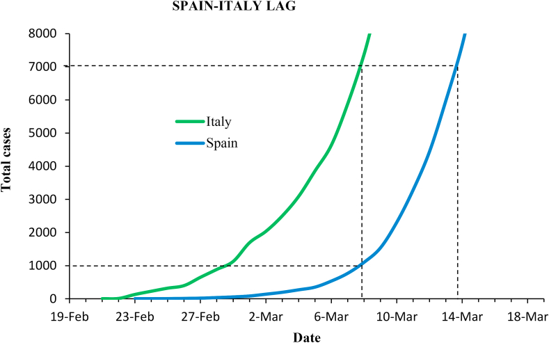
In this global context of pandemic, Spain experienced one of the worst situations. With a population of 47 million people, it has one of the highest rate of affected per million inhabitants, and one of the highest number of deaths per capita. Spain registered the first positive on 31 January 2020, from a German tourist in Canary Islands. Throughout February, Spain confirmed multiple cases related to the Italian cluster. On late February, the transmission was classified as local. In mid-March, cases had been registered in all 50 provinces, and Spain together with Italy were the most affected countries in the EU. On 14 March, a state of alarm and nationwide lockdown and quarantine were imposed to control the spread of the virus. Although Spain was seven days behind Italy in the outbreak, it did not enforced measures until it had more than 7,000 cases, the same than Italy the week before. On 3 April Spain surpassed Italy in total cases. After two months of strict containment measures, the epidemic was apparently under control, and from 14 May Spain began easing measures (NCE, 2020).
In this article, we study the Covid-19 outbreak in Spain, with a double objective: first, to explain the dynamics of the epidemic with the simplest possible model, and, second, to draw some lessons from a mathematical perspective that may be helpful to better understand the growth of an epidemic and to implement control measures. We use a deterministic SIR model, as well as a SEIR equivalent model, to describe the spread of the disease during the three and a half months from the start of the outbreak to its stabilization in Spain. We advocate the simplicity of the model as an advantage to effectively account for the coronavirus epidemic. From determination of a single parameter, the growth rate, we successfully simulate the epidemic curve and make predictions. As the method is directly applicable to other countries, we also study the case of Italy and Germany for comparison. After estimating the reproductive number, we discuss the feasibility of mitigation strategies and then evaluate the effectiveness of the suppression measures adopted in Spain. Likewise, we simulate scenarios to explore the potential impact of variations in the effectiveness. Finally, in this work we present simple analytical expressions that allow, by a simple calculation, to estimate the final size of the outbreak and the benefit of early intervention. This approach could help governments nowcasting the behavior of the outbreaks and designing adequate and prompt containment measures.
2. Methods
2.1. Deterministic SIR model and early growth dynamics
We used a susceptible-infectious-recovered SIR model (Kermack & McKendrick, 1927) to simulate the epidemic:
| (1) |
where , , and were the number of susceptible, infectious, and removed individuals at time t, and N is the total population, so . The coefficients denote: , reproductive number; , average infection period; , transmission (or infection) rate; and , removal rate. The simulation was based on the hypotheses: a) homogenous population, b) the whole population was susceptible, c) removed patients would be no longer infectious, d) infectivity was constant, and e) there was only human-to-human transmission with no zoonotic transmission.
Since the outbreak progression remains under the early growth dynamics, the approximation holds and the growth is purely exponential:
| (2) |
where is the initial infected population, and is the Malthusian coefficient for the exponential growth rate, defined as the solution to the Euler–Lotka equation (Britton & Tomba, 2019):
| (3) |
From Eqs. (1), (2), the removed population is obtained by integration (Appendix A):
| (4) |
2.2. Equivalent SEIR model
We also used a susceptible-exposed-infectious-recovered SEIR model, with governing equations
| (5) |
where , , , and were the number of susceptible, exposed or latent (infected but not yet infectious), infectious, and removed individuals at time t, was the infection period, and the latent period.
The solution of the differential equations yields (Appendix B)
| (6) |
where
| (7) |
and the subindex 1 corresponds to the positive sign in the solution. The growth rate is . Therefore, the early SEIR dynamics is equivalent to the exponential growth obtained with the SIR model choosing properly the parameters:
| (8) |
2.3. Epidemiological constants
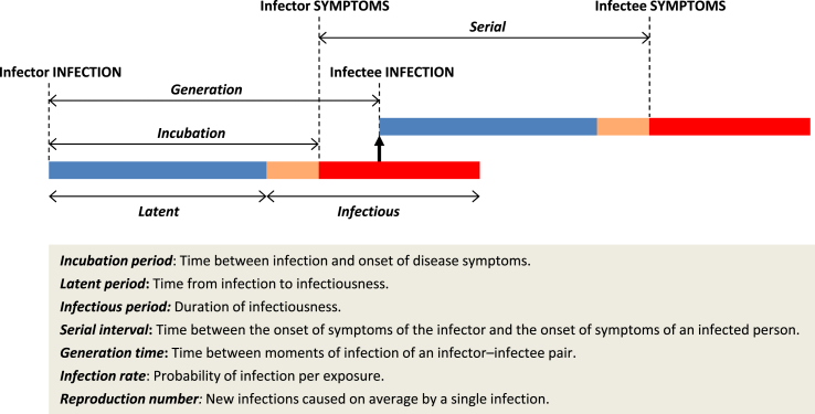
Definitions of epidemiological concepts in connection with mathematical well-defined parameters are often not obvious (Svensson, 2007). Fig. (1) shows the definitions of some epidemic metrics as well as a graphical interpretation. Although the incubation period (time until symptoms) is usually assumed to be similar to the latent period, the novel coronavirus is believed to be infectious during incubation before onset of symptoms (Du et al., 2020; Nishiura et al., 2020), so the serial interval is close to the incubation period. Recent studies (see review in Table 1) showed that the serial interval of COVID-19 ranges between 4 and 8 days, with average of 6 days, and the incubation period is between 2 and 14 days, with average of 5.5 days.
Fig. 1.
Epidemic metrics and graphical interpretation.
Table 1.
Review of epidemiological constants and parameters for SARS-CoV-2.
| Reproductive number | Infection rate (days−1) | Infectious period (days) | Incubation period (days) | Latent period (days) | Serial interval (days) | Ref. |
|---|---|---|---|---|---|---|
| 1.4–2.5 | 7 | WHO (2020) | ||||
| 2.8–3.3 | 5–6 | ECDC (2020) | ||||
| 3.3 | Liu et al. (2020) | |||||
| 1.9–6.5 | 4–6 | 5.3 (4–8) | Park et al. (2020) | |||
| 2.4 (2–2.6) | 5.1 | 6.5 | Ferguson et al. (2020) | |||
| 2.7 (China) | 2.4 | 6 | 6 | 8.4 | Wu et al. (2020) | |
| 2.2 (China) | 5.2 | 7.5 ± 3.4 | Li et al. (2020) | |||
| 3.6–4.6 (China) | 0.8 | 4 | 4 | Choi and Ki (2020) | ||
| 6.5 (China) | 0.2 | 3 | 7 | Tang et al. (2020) | ||
| 2.8 (China) | 0.6–1.7 | 5 | 3 | Lin et al. (2020) | ||
| 1.6–2.6 (China) | 5.2 | Kucharski et al. (2020) | ||||
| 1.5–5.9 (China) | 0.3 | Zhao and Chen (2020) | ||||
| 2–3 (Spain) | Abbott et al. (2020) | |||||
| 2.9 Spain | Caicedo et al. (2020) | |||||
| 2.8–3.3 (Italy) | Remuzzi and Remuzzi (2020) | |||||
| 1-4 Italy | 2.3 | 5.2 | Distante et al. (2020) | |||
| 3 (Italy) | Abbott et al. (2020) | |||||
| 2.1–4.2 (Latin America) | Caicedo et al. (2020) | |||||
| 1 | 10.3 | 7 | Fang et al. (2020) | |||
| 5 (2–14) | Linton et al. (2020) | |||||
| 3–7 | Wang et al. (2020) | |||||
| 5 | Nishiura et al. (2020); You et al. (2020) | |||||
| 5.2 | 5.1 | Zhang et al. (2020) | ||||
| 1.4–6.5 (mean 3) | 0.2–1.7 | 2.3–10.3 (mean 4.6) | 2–14 (mean 5.5) | 3–7 (mean 5) | 4–8 (mean 6) | Range |
In SEIR models the latent period () and the infectious period () appears as fitting parameters, or as constants related with real values that are difficult to measure. In SIR models the infection period may be interpreted as the generation time () (Britton & Tomba, 2019; Svensson, 2007).
Typically, what we observe is not the infection transmission but the clinical onsets (symptoms), i.e. the serial interval (). Although the relationship between and is model-dependent, both have the same mean (Britton & Tomba, 2019). For this reason, we used the serial time as a proxy for the generation time (Fine, 2003):
| (9) |
and we took the average value of 6 days for the serial interval found in the literature review.
2.4. Parameters for the baseline scenario
Growth parameters were inferred from case-incidence reports (Dimitrov & Meyers, 2020; Lipsitch et al., 2003; Wallinga & Lipsitch, 2007). We fixed the removal rate by interpreting as the mean generation time, or serial interval, for COVID-19 ( = 6 days, see Section 2.3). From Eqs. (1), (2) the new daily cases reported are at time t. We linearized this expression to get
| (10) |
Then, the exponential growth rate is obtained from Eq. (10) by least-mean-square fitting of the observations . The reproductive number was calculated (Dimitrov & Meyers, 2020; Ridenhour et al., 2014) as
| (11) |
and the doubling time as
| (12) |
2.5. Outbreak data
Time-series data were obtained from the Ministry of Health of the Government of Spain through the daily reports published by the Health Alert and Emergency Coordination Centre, Ministry of Health (HAECC, 2020), and the National Centre of Epidemiology, Carlos III Health Institute (NCE, 2020).
In the case of Italy and Germany the source of information was the Italian Ministero della Salute (MSI, 2020), the Robert Koch Institut in Germany (RKI, 2020), and the WHO (2020).
2.6. Scenarios after intervention
We simulated the outbreak trend in Spain after the government-issued containment measures, assuming that the transmissibility (rate a) was reduced by 60%, 65%, 70%, 75%, and 80% after lockdown. Since no intensive testing nor contact tracing were implemented in Spain, we kept the removal rate fixed (b = 1/6 days−1). These simulated scenarios correspond to reproductive numbers from 1 to 0.5. Also long-term mitigation scenarios were simulated with r above 1.
The reproductive number after the intervention is
| (13) |
where E is the effectiveness of the measures. Only when falls below 1 (negative growth rate) the epidemic would fade out. Thus, the minimum value of the effectiveness to control the epidemic is
| (14) |
It can be shown (Appendix C) that the total affected population at the end of the epidemic is
| (15) |
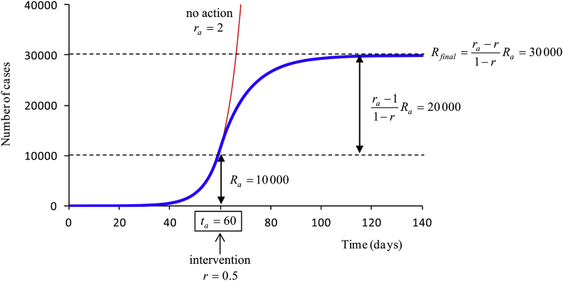
where is the number of affected people when the containment measures take effect, and the reproductive number at that time (Fig. 2).
Fig. 2.
Example of analytical estimation of the total affected population at the end of the epidemic. In this example, the reproductive number is 2 and there are 10,000 cases when control measures are enforced.
We also demonstrate in Appendix C that the total affected population reduces by the factor
| (16) |
if the intervention is performed days before, where is the growth rate at the moment of the intervention.
2.7. Nowcasting and forecasting
Assuming daily time increments, the instantaneous growth rate was calculated as
| (17) |
Time-varying estimates of the growth rate and the reproductive number were made by computing the weighted moving average (WMA) with a 6-day sliding window (Abbott et al., 2020). Rates obtained from this nowcasting were used to forecast the epidemic curve with the SIR model.
2.8. Confidence intervals
Results were expressed as the estimate of the parameter plus/minus the standard error. A confidence interval (CI) of 95% was also reported. The coefficient of determination, , was calculated in lineal regressions.
2.9. Model performance
The goodness-of-fit of the model was evaluated by means of two different statistics:
a) The root-mean-squared-error, as a measure of the residuals, defined as
| (18) |
where and are the real total cases and the total cases predicted with the model, respectively.
b) The coefficient of determination, defined as
| (19) |
where is the mean value of the total cases. This metric measures the proportion of the variance in the observations that is predictable from the model.
2.10. Software
Solving of differential equations, data fitting and parameters calculations were performed in MATLAB software, v 6.5 (The MathWorks, Inc., Natick, MA, USA), by using the statistical toolbox and custom-written routines.
3. Results
3.1. The outbreak dynamics in Spain
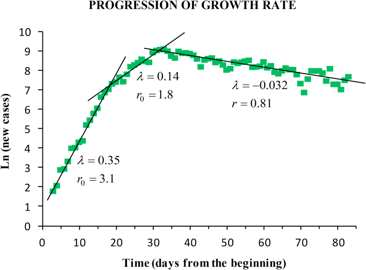
The baseline scenario lasted from the outbreak onset (23 February) until the incidence peak, which arrived on March 26. A delay of 12 days was observed from the start of containment measures (on March 15) to the peak. The fitting of the time-series yielded: average growth rate (95% CI 0.23–0.27; ), doubling time (95% CI 2.6–3.0), basic reproductive number (95% CI 2.3–2.7), and infection rate coefficient (95% CI 0.40–0.44). We estimated a number of 14 infectious people by February 21. During the one-month baseline period the exponential growth showed two different phases (Fig. 3). Until 11 March the epidemic grew faster, with (95% CI 0.33–0.37; ), infection rate (95% CI 0.50–0.54), and doubling time (95% CI 1.8–2.2). The instantaneous reproductive number during this early phase ranged from 2.6 to 3.6, with average (95% CI 2.9–3.3). Between March 12 and 26 March the epidemic began to spread to other regions. Growth rate was (95% CI 0.12–0.16; ), infection rate (95% CI 0.28–0.32), and doubling time (95% CI 4.2–5.8). Reproductive number during this second phase ranged from 1.5 to 2.9, with average (95% CI 1.6–2.0).
Fig. 3.
Lineal fitting of the logarithm of the daily new cases. The progression of the outbreak in Spain showed two phases of exponential growth (baseline scenario), and a steady exponential decrease during the lockdown. The fitting yields the growth rate (days−1) and the reproductive number.
During the lockdown after the incidence peak, the exponential decrease showed a fairly steady behaviour with negative growth rate (95% CI ; ), and average reproductive number (95% CI 0.77–0.85).
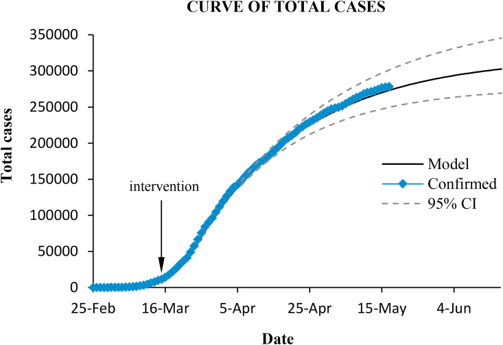
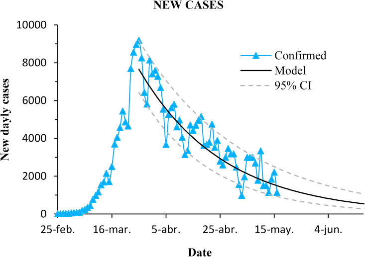
Fig. (4) and Fig. (5) show the cumulative and the daily confirmed cases in Spain, and the curves predicted with the SIR model by using the inferred parameters for the three main stages of the epidemic ( until 12 March; March 12–26; from March 27 onwards).
Fig. 4.
Total confirmed cases in Spain and prediction with the model. Dashed lines enclose the 95% confidence interval.
Fig. 5.
Progression of new daily cases in Spain and prediction with the model. Dashed lines enclose the 95% confidence interval.
The model performs quite well. The coefficient of determination of the prediction was , and the RMSE was 2.8%.
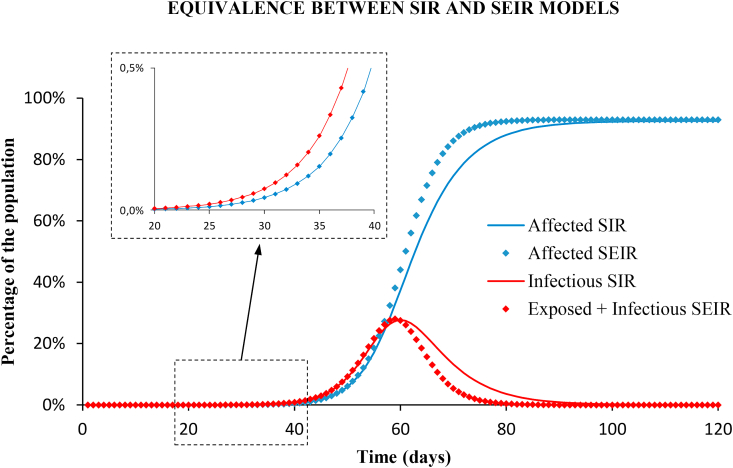
3.2. Equivalence between SIR and SEIR models
Fig. (6) shows the long-term prediction with the SIR and the SEIR models using the parameters of the baseline scenario, with no control measures. The results are almost identical, both for the cumulative cases and for the infectious cases, until reaching the no-intervention peak, which is very far from the early growth interval studied. The root-mean-squared-error (RMSE) between the number of affected population calculated with the SEIR and the SIR models is below 0.01% in the exponential growth phase. Only in the long-term, the results with both models differ by a maximum value of 5% (see Appendix D), but this does not correspond to any of the studied scenarios of the epidemic.
Fig. 6.
Long term prediction with SIR (solid lines) and SEIR (diamonds) models, with no intervention. Blue: cumulative cases of affected people. Red: infectious (note that the infectious compartment of the SIR model is equivalent to the union of latent and infectious groups of the SEIR model). Results with both models are identical in the early growth as shown in the enlarged windows.
For the equivalent SEIR model two different sets of parameters were inferred from Eq. (7) for the latent and the infectious periods: , ; and , .
In order to choose between models, we used the Akaike Information Criterion (AIC) and the Bayesian Information Criterion (BIC) to score the SIR and the SEIR models when applied to the fitting of the total case series (see Appendix E for more details). The SEIR model fits the observations only slightly better than the SIR model, and it is more complex since has one parameter more. Both criteria resulted higher in the SEIR model than in the SIR: , and , which means that the SIR model is the preferred candidate.
3.3. Mitigation scenarios
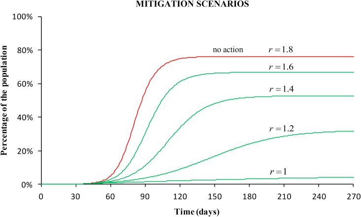
Fig. (7) shows the prediction of the total cases if a mitigation strategy had been adopted instead of strict confinement. At the time of the government intervention, the reproductive number was 1.8. Four mitigation scenarios are shown, corresponding to reproductive numbers 1.6, 1.4, 1.2, and 1. The final number of affected people would decrease to 67%, 53%, 32% and 4%, respectively. These numbers are still very large because of the high case-fatality of the disease (above 10% in Spain).
Fig. 7.
Simulation of four mitigation scenarios. The curves show the percentage of the affected population for decreasing reproductive numbers starting from 1.8 (value at the stage of the intervention) to 1. In these scenarios, the spread slows and population immunity builds up through the epidemic.
3.4. Suppression scenarios. Effectiveness of the containment measures
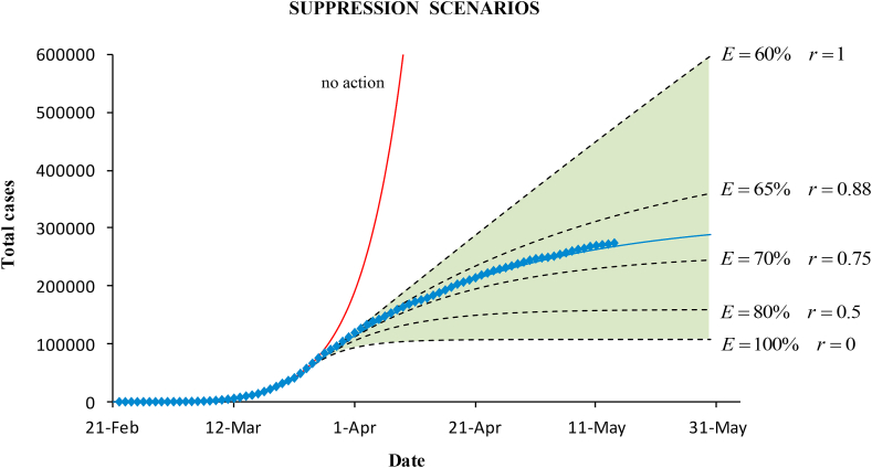
Simulations of suppression scenarios with reproductive numbers below 1 were made on March 27, when the government measures showed the effect. Knowing the baseline average reproductive number, , until March 26, the minimum value of the effectiveness to control the epidemic is . This means that strict containment measures, quarantine and lockdown, were necessary to reduce transmissibility.
Fig. (8) plots the cumulative cases for the different scenarios. The expected trend after the suppression should be within the shaded area limited by the minimum and the maximum effectiveness. Above mitigation would occur. The maximum suppression would be achieved with 100% effectiveness (). The actual confirmed cases and the epidemic modelled curve (for ) are also plotted. The effectiveness of the containment measures in Spain was 68%.
Fig. 8.
Epidemic curves for the cumulative cases obtained with the SIR model under different suppression scenarios (within the green shaded area). Simulations were made on March 27 by using the known baseline dynamics before control intervention, and potential values of the effectiveness of the containment measures.
3.5. Forecasting the final size of the epidemic
When containment measures started to show effect, the number of confirmed cases was , and the reproductive number . By using Eq. (15), we can predict the final number of cases at the end of the epidemic. Table 2 shows the results for the different scenarios after the intervention. The expected number in Spain is approximately 300,000. Results are the same as those obtained with the SIR simulation (Fig. 4). With this simple calculation, the projection in the long term is estimated. Even if the trend of the epidemic is not known a priori, these calculations anticipate what the variation range of the epidemic curve would be.
Table 2.
Final size (in total cases) for different effectiveness of the containment measures, and reduction factor depending on the anticipation time (, ,).
| E | r | (days) | ||
|---|---|---|---|---|
| 65% | 0.88 | 437,000 | 1 | 87% |
| 70% | 0.75 | 239,000 | 4 | 57% |
| 80% | 0.50 | 148,000 | 7 | 38% |
| 100% | 0 | 103,000 | 10 | 25% |
| 68% | 0.81 | 297,000 |
Because the dynamics is nonlinear, a small variation in effectiveness may produce a large difference in growth (Fig. 8) depending on the value of the reproductive number. Above 80% effectiveness (r below 0.5), the decay in total cases is very small; however, for r between 0.75 and 1, the final number of cases changes significantly.
3.6. Early action and reduction factor
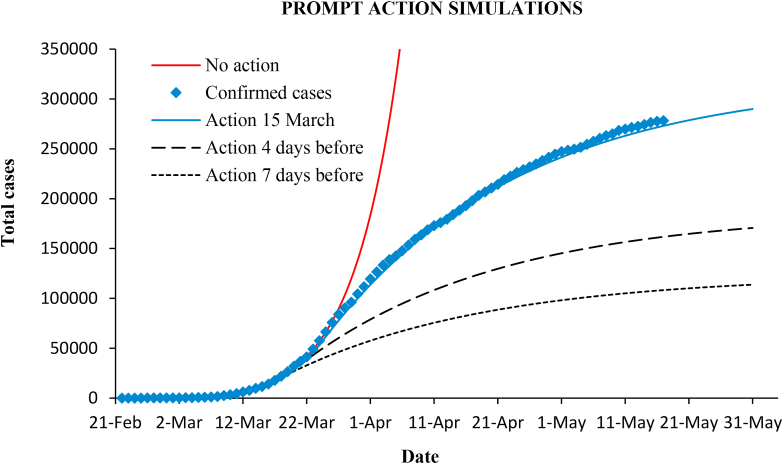
At best, with 100% effectiveness, the maximum suppression would drop the final epidemic size to . Due to the early exponential growth, increases as the intervention is delayed. Therefore, anticipation of control measures suppresses to a much greater degree. Fig. (9) shows simulations considering that measures in Spain had been enforced four or seven days before.
Fig. 9.
Epidemic curves simulation considering four or seven days of anticipation of the measures.
If the intervention is advanced days, the final cases reduce by the factor (Eq. (16)), where at the moment of the intervention. Thus, with = 4 and 7 days, the reduction of cases is 57% and 38%, respectively (as seen in Fig. 9). Table 2 also includes other reduction factors. For example, only one day in advance yields a reduction to 87%.
These results can also be interpreted in another way: prompt action allows enforcement of less severe measures with the same final result. For example, in the case of strong measures of 80% effectiveness to get the final cases (148,000) that would be reached is the same that in the case of lighter measures of 65% () if the intervention were 7.7 days before. Or, in the actual situation of Spain, the expected number of cases (297,000) would be the same having acted 7 days before with much less restrictive measures that drop r only to 0.94.
Spain was approximately one week behind Italy in the outbreak progression, as shown in Fig. (10). Italy recorded nearly 7,000 cases at the date of the government measures (March 8), while Spain counted only 1,000. Spain waited seven more days to act, and on March 15 cases had risen to nearly 10,000.
Fig. 10.
Epidemic curves in Italy and Spain before government-issued containment measures.
3.7. Comparison with Italy and Germany, and between Spanish regions
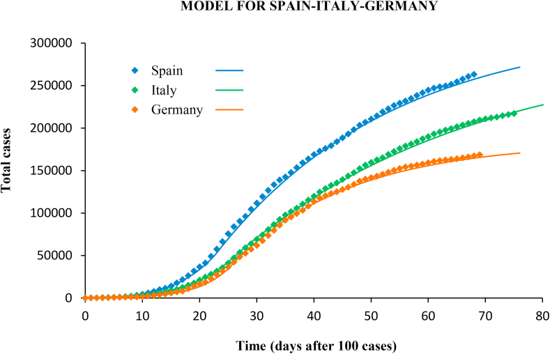
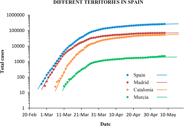
The same methodology was applied to the outbreak in Italy and Germany, and also in different regions in Spain. The confirmed cases and the modelled curves are plotted in Fig. 11, Fig. 12.
Fig. 11.
Confirmed cases (diamonds) and predictions (lines) with the SIR model for Spain, Italy and Germany.
Fig. 12.
Confirmed cases (diamonds) and predictions (lines) with the SIR model for different communities in Spain. The scale is logarithmic.
Italy implemented the government measures on March 8. The incidence peak occurred 13 days later. The average reproductive number before intervention was (95% CI 2.0–2.2), and, as in the case of Spain, the early growth of the epidemic showed two distinct phases with (until March 7) and 1.7 (8–21 March). Suppression measures lowered r to 0.86 (95% CI 0.84–0.88). In Germany the measures were implemented in several steps from March 13, with progressive closure of schools, travel restrictions, limitation of public activities, and curfew in some states. The incidence peak arrived on March 27. In the baseline the reproductive number changed from 3.4 (until March 7) to 2.1 (8–27 March), with average (95% CI 2.3–2.7). After government measures, r dropped to 0.72 (95% CI 0.68–0.76).
The model also performed well in the case of Italy and Germany, with a determination coefficient of in both cases, and RMSE of 2.2% and 2.8%, respectively.
The reproductive number in different communities in Spain shows a similar value, always around 2.5, although it is slightly lower (2.2) in Murcia than in the Community of Madrid and in Catalonia, which are more densely populated and with greater mobility. The containment measures have had a similar effectiveness and the reproductive number has dropped below 1 in all cases (Table 3).
Table 3.
Data of the outbreak in Spain, Italy, Germany, and three communities in Spain: Madrid, Catalonia and Murcia.
| Population | Spain |
Italy |
Germany |
Madrid |
Catalonia |
Murcia |
|---|---|---|---|---|---|---|
| 47M | 60M | 83M | 6.5M | 7.5M | 1.5M | |
| 2.5 | 2.1 | 2.5 | 2.5 | 2.5 | 2.2 | |
| 0.81 | 0.86 | 0.72 | 0.63 | 0.77 | 0.66 | |
| 100 cases | 1-Mar | 22-Feb | 28-Feb | 3-Mar | 10-Mar | 17-Mar |
| Intervention | 15-Mar | 8-Mar | 13-Mar | 15-Mar | 15-Mar | 15-Mar |
| Peak date | 26-Mar | 21-Mar | 27-Mar | 26-Mar | 28-Mar | 25-Mar |
4. Discussion and conclusions
We have proposed a simple and effective method to study the dynamics of the SARS-CoV-2 outbreak, based on the exponential growth and a SIR model. There is a plethora of epidemic models with different advantages and limitations: deterministic compartmental models, logistic and Gompertz models, likelihood-based methods, and stochastic simulations. Despite giving an overly simplified representation, deterministic models can describe the mechanisms in more detail (Ma, 2020). Among them the SEIR model is the most widely adopted for characterizing the COVID-19 epidemic (Fang et al., 2020; Kucharski et al., 2020; Lin et al., 2020; Tang et al., 2020; Wu et al., 2020). We have shown that the SIR and the SEIR models are equivalent by choosing the adequate parameters. A drawback to some models is they involve too many parameters (Ma, 2020). This can lead to an overfitting problem, when the model closely fits a data set but have poor predictive performance in other situations. Our SIR model is in good agreement with the epidemic in Spain as well as in other countries (Italy and Germany), and it has the advantage of being simple and including a single parameter.
We found two distinct phases in the one-month baseline scenario. The epidemic grew faster over the first two weeks (), and slower during the two following (). This was probably due to the strong initial expansion in the Community of Madrid, more populated and with greater mobility, followed by spread to other Spanish areas with less population density and, thus, lower transmissibility. As a result of the containment measures, the average growth rate dropped to . With only these three rates, we have predicted fairly well the epidemic curve with the SIR model over the entire period of more than two months until the stabilization of the curve.
The infection rate () in the baseline scenario is agreement with previous studies (Table 1). The average doubling time in Spain was 2.8 days (2.0 in the initial stage and 5.0 until the peak), which is consistent with the range 3–7 found in a review by Park et al. (2020). The latent and the infectious periods of the equivalent SEIR model (, ; and , ) are in the range found in the literature (Table 1).
We estimated an average of 2.5 for the basic reproductive number in the baseline scenario of the epidemic in Spain. The WHO (2020) reported an interval between 1.4 and 2.5 for the spread of coronavirus, the European Centre for Disease Prevention and Control (ECDC, 2020) a range from 2.8 to 3.3, and the Imperial College (Ferguson et al., 2020) a value of 2.4; Park et al. (2020) found 1.9–6.5 reviewing forty-one papers, and Liu et al. (2020) reported a mean of 3.3 from twelve works; in our own review for China we found 1.9–6.5; in Latin American countries values from 2.1 to 4.2 have been reported for the early stage (Caicedo et al., 2020). In the first two weeks, r in Spain was 3.1, in agreement with other studies of the epidemic in Spain: 2.7–3.1 during the first ten days (Caicedo et al., 2020), and 2–3 during the first two weeks (Abbott et al., 2020).
A limitation of the model is that we fixed the infection period by using the serial intervals from the literature. However, this would only affect the values of the reproductive number, but not the rest of the results and conclusions. We claim that it is possible to model the epidemic using only the growth rate. A value of 0 for this parameter indicates that the epidemic begins to fade up, which is equivalent to the value of 1 for the reproductive number regardless of the infection period.
Other limitations of our study have to do with the complexity and heterogeneity of the populations. In compartmental models, the account of the complex structure of the population requires increasing the number of compartments and defining the mixing between all the population subgroups in the model. Moreover, our mathematical model does not capture heterogeneity at the level of individual contacts, which could be important, for example, in super-spreading events. Finally, lockdown and social distancing do not have a total compliance, and the control measures may have different enforcement and observance in each territory. In our work, we have approached average populations.
Mitigation strategies may reduce the final size of the epidemic to between 70% and 4%, with the best case corresponding to reproductive number of 1 (60% transmissibility reduction), as also noted by Wu et al. (2020). In view of the high mortality rate of the disease, 6.8% worldwide and above 10% in Spain, it is unrealistic to wait for a major immunisation of the population and the “herd immunity” becomes at least controversial. A prevalence study has been conducted in Spain to determine how many people have developed antibodies after virus exposure. The results show that only 5% of Spaniards have been infected (ISCIII, 2020).
The proposed SIR model allows predictions to be made on the curve evolution and on the epidemic size under different scenarios according to the effectiveness of the suppression measures. These simulations are very useful, since they inform a priori about the benefit that the measures would provide depending on whether they were more or less strict, and also indicate to what extent they can relax without leaving the suppression scenarios. It is important to note that, due to the nonlinearity of the dynamics, a small variation in effectiveness will produce large changes in epidemic growth.
Throughout the suppression period we followed-up the instantaneous decrease rate and the reproductive number. We noticed that there is a delay of between 11 and 14 days from the implementation of the containment measures to the incidence peak, which is in agreement with the known reporting delay of about 14 days between infectiousness onset and confirmation (Lin et al., 2020). We found that quarantine measures in Spain played an important inhibitory effect on the outbreak, reducing the reproductive number to 0.81. The effectiveness of the containment measures was approximately 68%. This value is consistent with population mobility studies carried out with Big Data technology and mobile phone monitoring for the management of the COVID-19 crisis in Spain (INE, 2020), according to which mobility was reduced by between 60% and 80% during the lockdown. The effectiveness was similar across the country. However, Spain has started to gradually ease control measures in an asymmetric way because the epidemic reached different levels in each area. The effectiveness in Spain is lower than that achieved in China, where the reproductive number dropped to values of 0.5–0.75 (Zhao & Chen, 2020). Compared with other European countries in which the epidemic has developed approximately at the same time, the average reproductive number during the application of containment measures in Italy (0.86) and in Germany (0.72) has been similar to that of Spain, although the measures in Germany were not as strict than in Italy and Spain (ILO, 2020). In the UK, where the government first opted for mitigation and started later with lockdown measures, r stays at 1.
The reproductive number is a compound parameter. The best strategy to reduce transmissibility is the combination of measures that reduce the infection rate (such as lockdown and social distancing) with measures that reduce the infection period (by massive testing and contact tracing) (Guirao, 2020a; Nussbaumer-Streit et al., 2020). Spain and countries such as Italy have based their response on lockdown measures, which from a mathematical point of view means acting only on the reproductive number numerator. Thus, containment measures must be very strong, above 60%, to keep the epidemic within suppression scenarios. Furthermore, this carries a risk of rebound after easing measures (Guirao, 2020b).
Early action is critical. Spain was relatively slow to respond to the epidemic. A 7-day advance, based on the situation in Italy, in measures implementation would have reduced the impact to 40% in Spain.
This study applied to Spain, and in less detail to Italy and Germany, is useful to predict the trend of Sars-Cov-2 epidemic and provide a quantitative guide for other countries at high risk of outbreak. In addition to the epidemic curve modelling and predictions with the SIR or SEIR models, we have proposed two analytical formulas (Eqs. (15), (16))) that allows us to estimate with a simple calculation (without computing the dynamic equations) the final size of the epidemic in the predicted or other scenarios, and also the potential benefit that can be reached depending on when the control measures start. This provides a theoretical framework for the decision-making of epidemic interventions and prevention.
Declaration of competing interest
The authors declare that they have no known competing financial interests or personal relationships that could have appeared to influence the work reported in this paper.
Acknowledgments
This research is supported by a grant (project COV20/00736) from the Carlos III Health Institute, Ministry of Science and Innovation, Spain, in the framework of the Covid-19 Fund.
Handling editor: Dr. J Wu
Footnotes
Peer review under responsibility of KeAi Communications Co., Ltd.
Appendix A. Exponential growth in the SIR model
In the early growth dynamics and, thus, the equation for infectious
| (A.1) |
gives the solution
| (A.2) |
where is the initial infected population, and is the growth rate. Then, re-arranging the equation for removed gives
| (A.3) |
whose solution after integration is
| (A.4) |
where was the infectious period. Since the exponential function grows rapidly and (no initial removed population), we obtain:
| (A.5) |
That is
| (A.6) |
since .
Both populations grow exponentially but with lag :
| (A.7) |
Appendix B. Exponential growth in the SEIR model
Derivation of the equation for infectious gives
| (B.1) |
In the early growth dynamics , and the equation for exposed is
| (B.2) |
The solution of Eqs. (B.1–2) is
| (B.3) |
where
| (B.4) |
and and are the infection period and the latent period, respectively.
The Eq. (B.3) is the sum of two exponential functions with positive and negative exponents, and . The exponential with the negative exponent decays to zero rapidly. Thus, the exponential growths for the SEIR model are
| (B.5) |
| (B.6) |
| (B.7) |
The infectious group in the SIR model is equivalent to the sum of the infectious and exposed groups of the SEIR model: .
Appendix C. Epidemic size estimate after control measures, and effect of advancing the intervention
Let us consider the instant in which the suppression measures show the effect. At this moment the growth rate changes from to a negative rate , the reproductive number changes from to , and the number of affected people is . We establish this instant as the new origin of time. From there, the recovered people, Eq. (A.4), will follow the expression
| (C.1) |
As this function is a negative exponential, when the time is large enough we obtain
| (C.2) |
From Eq. (A.5):
| (C.3) |
where is the time elapsed from the beginning of the epidemic to the intervention. Therefore, if the measured are adopted days before, then the epidemic size reduces a factor
| (C.4) |
Appendix D. RMSE difference between models
The differences between the epidemic curves of the SEIR and the SIR models were measured with the root-mean-squared-error:
| (D.1) |
where and are the affected total population, calculated with the SEIR and the SIR models, respectively.
Fig. 13.
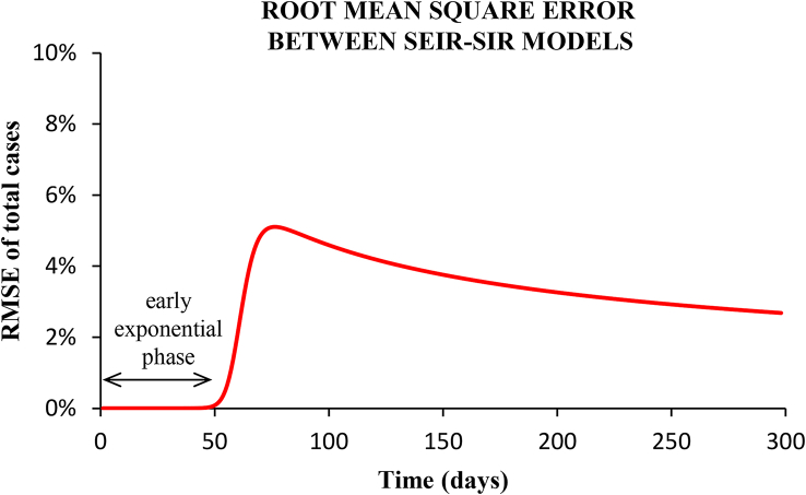
Root-mean-squared-error between the epidemic curves shown in Fig. (6) for the SEIR and the SIR models.
Fig. (13) plots the RMSE as a function of the period of time taken. In the early exponential growth phase, corresponding to the scenarios studied, the difference between models is practically zero (RMSE < 0.01%). Up to the incidence peak (with no-intervention), the RMSE is 0.2%. In the phase of decreasing incidence, the RMSE presents a maximum value of 5%, and afterwards the two epidemic curves converge again (see Fig. 6).
Appendix E. Information criteria for model comparison
In order to compare the relative quality of the models, the Akaike Information Criterion and the Bayesian Information Criterion were used in this paper. These estimators pose the trade-off between the goodness of the fit to the observations and the simplicity of the model. Both criteria include a penalty that is an increasing function of the number of estimated parameters, and that deals with complexity and the risk of overfitting.
The Akaike Information Criterion is defined as (Akaike, 1974)
| (E.1) |
and the Bayesian Information Criterion is defined as (Schwarz, 1978)
| (E.2) |
where k is the number of parameters estimated by the model, n the number of observations, and L the maximum likelihood.
Given a set of models, the preferred model is the one with the minimum AIC or BIC value.
References
- Abbott S., Hellewell J., Munday J.D., Chun J.Y., Thompson R.N., Bosse N.I., Chan Y.W.D., Russell R.W., Jarvis C.I., CMMID nCov working group, Flasche S., Kucharski A.J., Eggo R.M., Funk S. Temporal variation in transmission during the COVID-19 outbreak. 2020. https://cmmid.github.io/topics/covid19/current-patterns-transmission/global-time-varying-transmission.html/
- Akaike H. A new look at the statistical model identification. IEEE Trans. Automat. Contr., AC- 1974;19:716–723. [Google Scholar]
- Britton T., Tomba G.S. Estimation in emerging epidemics: Biases and remedies. Journal of The Royal Society Interface. 2019;16:20180670. doi: 10.1098/rsif.2018.0670. [DOI] [PMC free article] [PubMed] [Google Scholar]
- Caicedo-Ochoa Y., Rebellón-Sánchez D.E., Peñaloza-Rallón M., Cortés-Motta H.F., Méndez-Fandiño Y.R. Effective Reproductive Number estimation for initial stage of COVID-19 pandemic in Latin American Countries. International Journal of Infectious Diseases. 2020;95:316–318. doi: 10.1016/j.ijid.2020.04.069. [DOI] [PMC free article] [PubMed] [Google Scholar]
- Choi S.C., Ki M. Estimating the reproductive number and the outbreak size of COVID-19 in Korea. Epidemiology and Health. 2020;42 doi: 10.4178/epih.e2020011. [DOI] [PMC free article] [PubMed] [Google Scholar]
- Dimitrov N.B., Meyers L.A. Mathematical approaches to infectious disease prediction and control. Tutorials in operations research, informs 2020. 2020. [DOI]
- Distante C., Piscitelli P., Miani A. Covid-19 outbreak progression in Italian regions: Approaching the peak by the end of March in northern Italy and first week of April in southern Italy. International Journal of Environmental Research and Public Health. 2020;17:3025. doi: 10.3390/ijerph17093025. [DOI] [PMC free article] [PubMed] [Google Scholar]
- Dong E., Du H., Gardner L. An interactive web-based dashboard to track COVID-19 in real time. The Lancet Infectious Diseases. 2020;20(5) doi: 10.1016/S1473-3099(20)30120-1. [DOI] [PMC free article] [PubMed] [Google Scholar]
- Du Z., Xu X., Wu Y., Wang L., Cowling B.J., Meyers L.A. Serial interval of COVID-19 among publicly reported confirmed cases. Emerging Infectious Diseases. 2020;26(6):1341–1343. doi: 10.3201/eid2606.200357. [DOI] [PMC free article] [PubMed] [Google Scholar]
- ECDC, European Centre for Disease Prevention and Control Coronavirus disease 2019 (COVID-19) in the EU/EEA and the UK –8thupdate. 2020. https://www.ecdc.europa.eu/
- Fang Y., Nie Y., Penny M. Transmission dynamics of the COVID-19 outbreak and effectiveness of government interventions: A data-driven analysis. Journal of Medical Virology. 2020;92(6):645–659. doi: 10.1002/jmv.25750. [DOI] [PMC free article] [PubMed] [Google Scholar]
- Ferguson N.M., Laydon D., Nedjati-Gilani G., Imai N., Ainslie K., Baguelin M., Bhatia S., Boonyasiri A., Cucunubá Z., Cuomo-Dannenburg G., Dighe A., Dorigatti I., Fu H., Gaythorpe K., Green W., Hamlet A., Hinsley W., Okell L.C., van Elsland S., Ghani A.C. Impact of non-pharmaceutical interventions (NPIs) to reduce COVID19 mortality and healthcare demand. Imperial College COVID-19 Response Team, Report 9. 2020. [DOI]
- Fine P.E.M. The interval between successive cases of an infectious disease. American Journal of Epidemiology. 2003;158(11):1039–1047. doi: 10.1093/aje/kwg251. [DOI] [PubMed] [Google Scholar]
- Guirao A. Entender una epidemia. El coronavirus en España, situación y escenarios. Revista Española de Física. 2020;34(2):3–10. [Google Scholar]
- Guirao A. 2020. Follow-up of the epidemic in Spain.https://www.um.es/phi/aguirao/Covid19/ [Google Scholar]
- HAECC, Health Alert and Emergency Coordination Centre, Ministry of Health Information on the outbreak of pneumonia caused by a new coronavirus (COVID-19) 2020. https://www.mscbs.gob.es/
- Hopkins University J. COVID-19 dashboard by the center for systems science and engineering (CSSE) 2020. https://coronavirus.jhu.edu/map.html/
- ILO, International Labour Organization COVID-19 and the world of work. Country policy responses. 2020. https://www.ilo.org/global/topics/coronavirus/country-responses/
- INE, Ministerio de Transporte y Movilidad, Gobierno de España . Instituto Nacional de Estadística (INE),; 2020. Análisis de la movilidad en España durante el estado de alarma.https://www.mitma.gob.es/ministerio/covid-19/https://www.ine.es/covid/covid_movilidad.htm/ [Google Scholar]
- ISCIII, Instituto de Salud Carlos III, Ministerio de Sanidad, Gobierno de España ENE-COVID19. Estudio nacional de sero-epidemiología de la infección por Sars-Cov-2 en España. 2020. https://portalcne.isciii.es/enecovid19/
- Kermack W.O., McKendrick A.G. A contribution to the mathematical theory of epidemics. Proceedings of the Royal Society of London A. 1927;115:700–721. [Google Scholar]
- Kucharski A.J., Russell T.W., Diamond C., Liu Y., Edmunds J., Funk S., Eggo R.M. Early dynamics of transmission and control of COVID-19: A mathematical modelling study. The Lancet Infectious Diseases. 2020;20:553–558. doi: 10.1016/S1473-3099(20)30144-4. [DOI] [PMC free article] [PubMed] [Google Scholar]
- Li Q., Guan X., Wu P., Wang X., Zhou L., Tong Y., Ren R., Leung K.S.M., Lau E.H.Y., Wong J.Y., Xing X., Xiang N., Wu Y., Li C., Chen Q., Li D., Liu T., Zhao J., Liu M., Feng Z. Early transmission dynamics in wuhan, China, of novel coronavirus infected pneumonia. New England Journal of Medicine. 2020;382(13):1199–1207. doi: 10.1056/NEJMoa2001316. [DOI] [PMC free article] [PubMed] [Google Scholar]
- Linton N.M., Kobayashi T., Yang Y., Hayashi K., Akhmetzhanov A.R., Jung S., Yuan B., Kinoshita R., Nishiura H. incubation period and other epidemiological characteristics of 2019 novel coronavirus infections with right truncation: A statistical analysis of publicly available case data. Journal of Clinical Medicine. 2020;9:538. doi: 10.3390/jcm9020538. [DOI] [PMC free article] [PubMed] [Google Scholar]
- Lin Q., Zhao S., Gao D., Lou Y., Yang S., Musa S.S., Wang M.H., Cai Y., Wang W., Yang L., He D. A conceptual model for the coronavirus disease 2019 (COVID-19) outbreak in Wuhan, China with individual reaction and governmental action. International Journal of Infectious Diseases. 2020;93:211–216. doi: 10.1016/j.ijid.2020.02.058. [DOI] [PMC free article] [PubMed] [Google Scholar]
- Lipsitch M., Cohen T., Cooper B., Robins J.M., Ma S., James L., Gopalakrishna G., Chew S.K., Tan C.C., Samore M.H., Fisman D., Murray M. Transmission dynamics and control of severe acute respiratory syndrome. Science. 2003;300(5627):1966–1970. doi: 10.1126/science.1086616. [DOI] [PMC free article] [PubMed] [Google Scholar]
- Liu Y., Gayle A.A., Wilder-Smith A., Rocklöv J. The reproductive number of COVID-19 is higher compared to SARS coronavirus. Journal of Travel Medicine. 2020;27:1–4. doi: 10.1093/jtm/taaa021. [DOI] [PMC free article] [PubMed] [Google Scholar]
- Ma J. Estimating epidemic exponential growth rate and basic reproduction number. Infectious Disease Modelling. 2020;5:129–141. doi: 10.1016/j.idm.2019.12.009. [DOI] [PMC free article] [PubMed] [Google Scholar]
- MSI, Ministero della Salute, Italia Covid-19 - situazione in italia. 2020. http://www.salute.gov.it/nuovocoronavirus/
- NCE, National Centre of Epidemiology, Carlos III Health Institute, Ministry of Science and Innovation COVID-19 in Spain. 2020. https://cnecovid.isciii.es/
- Nishiura H., Linton N.M., Akhmetzhanov A.R. Serial interval of novel coronavirus (COVID-19) infections. International Journal of Infectious Diseases. 2020;93:284–286. doi: 10.1016/j.ijid.2020.02.060. [DOI] [PMC free article] [PubMed] [Google Scholar]
- Nussbaumer-Streit B., Mayr V., Dobrescu A.I., Chapman A., Persad E., Klerings I., Wagner G., Siebert U., Christof C., Zachariah C., Gartlehner G. Quarantine alone or in combination with other public health measures to control COVID-19: A rapid review. Cochrane Database of Systematic Reviews. 2020;4 doi: 10.1002/14651858.CD013574. [DOI] [PMC free article] [PubMed] [Google Scholar]
- Park M., Cook A.R., Lim J.T., Sun Y., Dickens B.L. A systematic review of COVID-19 epidemiology based on current evidence. Journal of Clinical Medicine. 2020;9(4):967–970. doi: 10.3390/jcm9040967. [DOI] [PMC free article] [PubMed] [Google Scholar]
- Remuzzi A., Remuzzi G. COVID-19 and Italy: What next? Lancet. 2020;395:1225–1228. doi: 10.1016/S0140-6736(20)30627-9. [DOI] [PMC free article] [PubMed] [Google Scholar]
- Ridenhour B., Kowalik J.M., Shay D.K. Unraveling R0: Considerations for public health applications. American Journal of Public Health. 2014;104:32–41. doi: 10.2105/AJPH.2013.301704. [DOI] [PMC free article] [PubMed] [Google Scholar]
- RKI, Robert Koch Institut . 2020. Coronavirus disease 2019 (COVID-19) daily situation report of the Robert Koch Institute Berlin.https://www.rki.de/EN/ [Google Scholar]
- Schwarz G. Estimating the dimension of a model. Annals of Statistics. 1978;6(2):461–464. [Google Scholar]
- Svensson A. A note on generation times in epidemic models. Mathematical Biosciences. 2007;208(1):300–311. doi: 10.1016/j.mbs.2006.10.010. [DOI] [PubMed] [Google Scholar]
- Tang B., Wang X., Li Q., Bragazzi N.L., Tang S., Xiao Y., Wu J. Estimation of the transmission risk of the 2019-nCoV and its implication for public health interventions. Journal of Clinical Medicine. 2020;9(2):462. doi: 10.3390/jcm9020462. [DOI] [PMC free article] [PubMed] [Google Scholar]
- Wallinga J., Lipsitch M. How generation intervals shape the relationship between growth rates and reproductive numbers. Proceedings Biological Sciences. 2007;274(1609):599–604. doi: 10.1098/rspb.2006.3754. [DOI] [PMC free article] [PubMed] [Google Scholar]
- Wang C., Horby P.W., Hayden F.G., Gao G.F. A novel coronavirus outbreak of global health concern. Lancet. 2020;395:470–473. doi: 10.1016/S0140-6736(20)30185-9. [DOI] [PMC free article] [PubMed] [Google Scholar]
- WHO, World Health Organization Coronavirus disease (COVID-19) pandemic. 2020. https://www.who.int/emergencies/diseases/novel-coronavirus-2019/
- Worldometers 2020. https://www.worldometers.info/coronavirus/
- Wu J.T., Leung K., Leung G.M. Nowcasting and forecasting the potential domestic and international spread of the 2019-nCoV outbreak originating in wuhan, China: A modelling study. Lancet. 2020;395:689–697. doi: 10.1016/S0140-6736(20)30260-9. [DOI] [PMC free article] [PubMed] [Google Scholar]
- You C., Deng Y., Hu W., Sun J., Lin Q., Zhou F., Pang C.H., Zhang Y., Chen Z., Zhou X.H. Estimation of the time-varying reproduction number of COVID-19 outbreak in China. International Journal of Hygiene and Environmental Health. 2020;228:113555. doi: 10.1016/j.ijheh.2020.113555. [DOI] [PMC free article] [PubMed] [Google Scholar]
- Zhang J., Litvinova M., Wang W., Wang Y., Deng X., Chen X., Li M., Zheng W., Yi L., Chen X., Wu Q., Liang Y., Wang X., Yang J., Sun K., Longini I.M., Jr., Halloran M.E., Wu P., Cowling B.J., Yu H. Evolving epidemiology and transmission dynamics of coronavirus disease 2019 outside hubei province, China: A descriptive and modelling study. The Lancet Infectious Diseases. 2020;20:793–802. doi: 10.1016/S1473-3099(20)30230-9. [DOI] [PMC free article] [PubMed] [Google Scholar]
- Zhao S., Chen H. Modeling the epidemic dynamics and control of COVID-19 outbreak in China. Quantitative Biology. 2020;8(1):11–19. doi: 10.1007/s40484-020-0199-0. [DOI] [PMC free article] [PubMed] [Google Scholar]


