

Abstract
Sagittarius A* (Sgr A*) is the variable radio, near-infrared (NIR), and X-ray source associated with accretion onto the Galactic center black hole. We present an analysis of the most comprehensive NIR variability data set of Sgr A* to date: eight 24 hr epochs of continuous monitoring of Sgr A* at 4.5 μm with the IRAC instrument on the Spitzer Space Telescope, 93 epochs of 2.18 μm data from Naos Conica at the Very Large Telescope, and 30 epochs of 2.12 μm data from the NIRC2 camera at the Keck Observatory, in total 94,929 measurements. A new approximate Bayesian computation method for fitting the first-order structure function extracts information beyond current fast Fourier transformation (FFT) methods of power spectral density (PSD) estimation. With a combined fit of the data of all three observatories, the characteristic coherence timescale of Sgr A* is minutes (90% credible interval). The PSD has no detectable features on timescales down to 8.5 minutes (95% credible level), which is the ISCO orbital frequency for a dimensionless spin parameter a = 0.92. One light curve measured simultaneously at 2.12 and 4.5 μm during a low flux-density phase gave a spectral index αs = 1.6 ± 0.1 . This value implies that the Sgr A* NIR color becomes bluer during higher flux-density phases. The probability densities of flux densities of the combined data sets are best fit by log-normal distributions. Based on these distributions, the Sgr A* spectral energy distribution is consistent with synchrotron radiation from a non-thermal electron population from below 20 GHz through the NIR.
Keywords: accretion, accretion disks; black hole physics; Galaxy: center; methods: statistical; radiation mechanisms: non-thermal
1. Introduction
The broadband radiation source Sgr A* is located at the heart of the so-called S-star cluster (Sabha et al. 2012) at the center of the Milky Way. Sgr A*’s position is coincident with the dynamical center of the S-stars and therefore coincident with the dynamically derived location (to within ~2 mas) of the central supermassive black hole (SMBH) of our Galaxy (e.g., Yelda et al. 2010). That makes Sgr A* more than 100 times closer than any other supermassive black hole (SMBH), and it can therefore be studied in far greater detail.
Sgr A* is visible as a compact, moderately variable radio source having flux densities between 0.5 and 4 Jy in the range 0.1 to 360 GHz (Balick & Brown 1974; Falcke et al. 1998; Falcke & Markoff 2000; Zhao et al. 2001; Herrnstein et al. 2004; Miyazaki et al. 2004; Mauerhan et al. 2005; Yusef-Zadeh et al. 2006b, 2009; Marrone et al. 2008; Li et al. 2009; Kunneriath et al. 2010; García-Marín et al. 2011; Bower et al. 2015; Rauch et al. 2016; Capellupo et al. 2017). Sgr A* has much dimmer NIR and X-ray counterparts that are variable by up to 30 times the mean flux density in the NIR and up to a factor 500 in the X-rays (Baganoff et al. 2001; Hornstein et al. 2002; Genzel et al. 2003; Ghez et al. 2004; Eisenhauer et al. 2005; Hornstein et al. 2007; Meyer et al. 2008; Porquet et al. 2008; Do et al. 2009; Dodds-Eden et al. 2009, 2011; Sabha et al. 2010; Witzel et al. 2012; Neilsen et al. 2013, 2015; Ponti et al. 2017; Zhang et al. 2017). The X-ray energy output can become comparable to the submm level during the brightest flares. This strong, rapid variability may be associated with accretion processes close to the supermassive black hole’s event horizon. The connection of the variability to regions close to the event horizon is based on (1) the observed timescales of the variability, with common changes of a factor ≳10 within ~10 minutes in the NIR (Genzel et al. 2003; Ghez et al. 2004); (2) the spectral index10 αs ≈ 0.6 (Ghez et al. 2005a; Hornstein et al. 2007; Bremer et al. 2011; Witzel et al. 2014); (3) linear polarization in the NIR and submm (Eckart et al. 2006b; Marrone et al. 2006, 2007; Meyer et al. 2006b; Trippe et al. 2007; Yusef-Zadeh et al. 2007; Eckart et al. 2008a; Nishiyama et al. 2009; Witzel et al. 2011; Shahzamanian et al. 2015); and (4) temporal correlations between the submm, NIR, and X-ray regimes. All of these observational results point to a population of relativistic electrons in a region that is smaller than ~10 light minutes (the distance associated with the light crossing time, <15 Schwarzschild radii) emitting synchrotron radiation at NIR wavelengths. The variable submm and X-ray radiation may be synchrotron emission or may be linked by radiative transfer processes such as adiabatic expansion and inverse Compton or synchrotron self-Compton scattering, respectively (Baganoff et al. 2001; Eckart et al. 2004; Yusef-Zadeh et al. 2006a, 2006b, 2008, 2009, 2012; Eckart et al. 2006a, 2008a, 2008b, 2012; Gillessen et al. 2006; Marrone et al. 2008; Dodds-Eden et al. 2009; Trap et al. 2011; Haubois et al. 2012; Dibi et al. 2016; Mossoux et al. 2016; Rauch et al. 2016; Ponti et al. 2017).
In order to shed light on the physical and radiative mechanisms at work and on the interrelation between wavelengths, many studies have attempted to find and categorize recurring patterns and regularities in the behavior of Sgr A*, both statistically for individual wavelength regimes as well as in the form of correlations between bands (Gillessen et al. 2006; Meyer et al. 2006a, 2006b, 2009, 2014, 2007; Hornstein et al. 2007; Do et al. 2009; Zamaninasab et al. 2010; Dodds-Eden et al. 2011; Witzel et al. 2012; Neilsen et al. 2013, 2015; Dexter et al. 2014; Hora et al. 2014; Subroweit et al. 2017). In recent years, the preponderance of studies has arrived at the following set of phenomenological but statistically rigorous results:
Sgr A* is a continuously variable NIR source that emits above the 2.12 μm detection level (0.05 mJy observed or 0.5 mJy dereddened, 3σ above the noise level of the NIRC2 camera at the Keck II telescope) ~90% of the time (Witzel et al. 2012; Meyer et al. 2014). Its probability density function (PDF) of flux densities11 at 2.18 μm is highly skewed (Dodds-Eden et al. 2011) and can be described by a power law with a slope βIR ≈ 4 (Witzel et al. 2012). The first three moments of the PDF are well defined with mean ≈5.8 mJy dereddened (≈0.6 mJy observed), variance ≈9.4 mJy2 dereddened, and skewness ≈52.3 mJy3 dereddened. The brightest observed NIR peak reached ~30 mJy (dereddened, Dodds-Eden et al. 2009). Peaks with F (2.18 μm) > 10 mJy (dereddened) occur about four times a day (Do et al. 2009; Meyer et al. 2009, 2014; Hora et al. 2014).
The X-ray emission comes from a steady, extended (~1″) source plus outbursts from an unresolved source. Outburst flux densities can be several hundred times the level of the quiescent state. Outbursts (frequently called “flares” in the literature) have the character of distinct events and occur about once per day. The unresolved source is detectable only during outbursts. At other times, fluctuations are sufficiently described by the Poisson distribution expected for the steady source (Neilsen et al. 2015). The flux-density PDF, as for the NIR, is well described by a power-law distribution but with βX ≈ 2. X-ray flares seem always to be accompanied by NIR peaks (Morris et al. 2012 and references therein). However, the reverse is not true, and only about one in four F(2.18 μm) > 10 mJy (dereddened) NIR peaks has an X-ray counterpart (Baganoff et al. 2001; Eckart et al. 2004; Marrone et al. 2008; Porquet et al. 2008; Do et al. 2009; Neilsen et al. 2013, 2015). There is no obvious relationship between X-ray and NIR flux-density levels.
The spectral energy distribution of Sgr A* peaks in the submm (Zylka et al. 1992, 1995; Falcke et al. 1998; Melia & Falcke 2001), where it is visible as a synchrotron source powered by the dominant thermal electron population (Yuan et al. 2003). An analysis by Dexter et al. (2014) of ~10 years of 1.3, 0.87, and 0.43 mm observations with CARMA and SMA shows a steady flux-density level of ~3 Jy with Gaussian fluctuations about that mean. Submm flux-density enhancements rising ~1 Jy above the mean occur approximately 1.2 times per day (Marrone et al. 2008). A time-series analysis of submm light curves gave a mean reversion timescale of ~8 hr (Dexter et al. 2014).
The patterns of correlation between wavelengths are still unclear. Several authors have suggested that the submm peaks often follow bright NIR peaks by 1–3 hr (Eckart et al. 2006a, 2008b, 2009, 2012; Yusef-Zadeh et al. 2006b, 2009, 2011; Marrone et al. 2008), but most observations remain inconclusive in this regard because of the lack of simultaneous multi-wavelength data of sufficient length and overlap. Indeed, there are counterexamples. Recent observations obtained with the Spitzer Space Telescope, the Chandra X-ray Observatory, the SMA, and the W. M. Keck Observatory suggest that the phenomenology of these correlations is not simple (Fazio et al. 2018). In particular, SMA and Spitzer observed the first example of an effectively synchronous sequence of variations in the submm and NIR. Another example obtained with SMA, Chandra, and Keck showed an even more surprising sequence in which a submm peak precedes an X-ray flare, which in turn was followed by a NIR peak. Albeit not conclusive due to the limitations of ground-based observations, such a sequence of peaks contradicts the canonical phenomenology of simultaneous X-ray and NIR followed by delayed submm variations.
There are many previous studies of the statistical properties of Sgr A*ʼs variability. Initially, these studies focused on putative quasi-periodicity (QPO) at timescales between 10 and 20 minutes and its relation to the innermost stable orbit of the 4 × 10⁶ M⨀ SMBH (Genzel et al. 2003; Meyer et al. 2006a, 2006b, 2007; Trippe et al. 2007; Zamaninasab et al. 2010; Karssen et al. 2017). Do et al. (2009) found no evidence for such a QPO based on available data at the time. Consequently, the scope of the statistical analysis was broadened with a determination of the red-noise correlation timescale ( minutes) in the NIR (Meyer et al. 2009) that allowed for a comparison of Sgr A* with black holes of different mass regimes. This comparison revealed that the mass and characteristic timescale of Sgr A* are consistent with a linear mass–timescale relation without a luminosity correction term as proposed by, for example, McHardy et al. (2006), who discussed characteristic timescales of AGN and black hole X-ray binaries (BHXRB). In this context, Meyer et al. (2009) pointed out the exceptional value of Sgr A* because it is the SMBH with the most precise mass determination so far: Mbh = (4.02 ± 0.16 ± 0.04) × 106 M⨀ (Boehle et al. 2016), where the error bar terms give the statistical and systematic uncertainties, respectively.
Another line of inquiry has considered the possibility of a dichotomy of the NIR variability into statistically different processes (or “states”) with either different flux-density PDFs or different timing behavior or both. These inquiries have been motivated by some NIR flares having X-ray counterparts while others do not (Dodds-Eden et al. 2011). The statistics of the variations have been shown to be consistent with a single variability state without evidence for multiple superimposed or interleaved variability processes (Witzel et al. 2012; Meyer et al. 2014).
A variety of NIR spectral index values have been reported. While some authors found a strong dependence of the spectral index on the flux-density level, other high-cadence and high-signal-to-noise studies at K-band-equivalent flux densities >0.2 mJy showed only minor intrinsic fluctuations around an H- (1.65 μm) to L-band (3.8 μm) spectral index αs = 0.6 (Ghez et al. 2005a; Eisenhauer et al. 2005; Gillessen et al. 2006; Krabbe et al. 2006; Hornstein et al. 2007; Bremer et al. 2011; Witzel et al. 2014).
Sgr A* is linearly polarized in the NIR. Shahzamanian et al. (2015) statistically analyzed time series and found typical polarization of (20 ± 10)% and a preferred position angle of (13 ± 15)°.
In summary, the NIR variability is well characterized as a red-noise process—that is, it has a power spectral density (PSD)12 that is a power law with a slope γ1 ≈ 2 for timescales in the range ~20 to ~150 minutes. The process is a damped random walk—that is, it has a correlation (or characteristic) timescale. For timescales longer than the correlation timescale ( minutes at the 90% credible level13; Meyer et al. 2009), the process is uncorrelated white noise, and the PSD becomes flat for the corresponding lowest frequencies (see Appendix B.1). Based on the available data sets, no evidence for periodicity, quasi-periodicity, or changes in its statistical behavior (e.g., a two-state variability model) could be found. In fact, the existing knowledge of the NIR variability of Sgr A* can be described statistically by as few as five parameters: the PSD slope and break timescale, the slope and normalization of the power-law flux-density PDF, and the NIR spectral index. Two more parameters are needed to describe the linear polarization: the fixed polarization fraction and position angle. Considering the large amplitudes of flux-density fluctuations, such constancy of statistical and physical parameters over the period of existing data is surprising.
Specific scenarios for producing NIR variability have invoked magnetic reconnection events, disk instabilities, ejection and expansion of plasma blobs, unsteady jet emission, or accretion of magnetic fields (Sharma et al. 2007; Dodds-Eden et al. 2010; Yuan & Bu 2010; Eckart et al. 2012). However, these theoretical efforts to model the turbulent accretion flow and the variability caused by the accretion cannot fully explain all observations to date. In particular, the peak NIR flux densities are higher than predicted by radiative transfer models of three-dimensional general relativistic magnetohydrodynamic (GRMHD) simulations with a thermal electron distribution function that matches millimeter flux densities. The observed NIR variability may therefore be due to the acceleration of electrons out of the dominant thermal component of the distribution function into a non-thermal tail (e.g., Dodds-Eden et al. 2010).
GRMHD models with a thermal electron distribution, while producing only relatively weak variability (Dolence et al. 2012), have an interesting feature in their power spectrum near fISCO, the orbital frequency of the innermost stable circular orbit (ISCO). In particular, these models show an approximately f −2 power spectrum at f < fISCO, a bump in power close to fISCO, and a break in the spectrum to approximately f −4 at f > fISCO. This is consistent with the notion that variability in the disk at frequencies above the orbital frequency is associated with disk turbulence, which is known from simulations to have a steeply declining spatial power spectrum (e.g., Guan et al. 2009). This would naturally give rise to a steeply declining temporal power spectrum as well. With Spitzer (Hora et al. 2014), in combination with ground-based 8–10 m telescopes, the predicted PSD short-timescale structure is testable.
This work presents the first analysis of the NIR PSD of Sgr A* that includes continuous data sets for all relevant timescales from 24 hr down to the sub-minute level. We use an unprecedented data set from three different observatories: the W. M. Keck Observatory, the European Southern Observatory Very Large Telescope (ESO/VLT), and the Spitzer Space Telescope. The observatories contribute complementary information about the PSD: the Keck data have the best signal-to-noise and can detect Sgr A* variations at timescales below 1 minute. A limitation is that most of the Keck data sets have a duration of ⩽2 hr. The VLT data cover timescales between 4 minutes and 6 hr, and the Spitzer data timescales from ~7 minutes to 24 hr, much longer than the previously derived correlation timescale. Together, these data enable the most precise estimate possible today of the correlation timescale and a test for PSD features at timescales below 50 minutes.
To exploit the combined data sets, we have developed an entirely new algorithm. It uses the first-order structure function as the central tool for analyzing the timing of Sgr A* and a customized population Monte Carlo approximate Bayesian computation (PMC-ABC) sampler to derive parameter values. The goals of this paper are to
provide this extensive data set to the community with a full statistical characterization;
introduce the new PMC-ABC algorithm that will have wide application to variable sources;
determine the PSD of the variability process of Sgr A*, including a new determination of the correlation timescale;
determine the Sgr A* flux-density PDF in both K- and M-band (4.5 μm);
characterize the Sgr A* spectral index between these two bands; and
characterize the instrumental performance of this kind of space-based variability study in comparison to ground-based AO telescopes.
Section 2 describes the observations and data sets used in this work. Section 3 and Appendix B present the newly developed algorithm for analyzing non-deterministic stationary linear time series and the results of our analysis of the Sgr A* light curves. Sections 4 and 5 discuss the results and present our conclusions. Readers mainly interested in the mathematical foundation of our methodology are referred to Appendices B–D. Readers only interested in our main results are refereed to Figures 10, 13, 17, and 19, and Tables 5 and 6.
Figure 10.

Results of the Bayesian structure function fit for Case 3 (log-normal/log normal; see Section 3). Contours show the joint (posterior) probability density for each parameter pair, and panels along the upper right edge show histograms of the marginalized posterior of each parameter defined in Table 5. For each histogram, the dashed lines mark the 16%, 50%, and 84% quantiles. Upper limit for 1/fb,2 with a probability of 95% is 8.5 minutes, about the same as Cases 1 and 2.
Figure 13.

Credible contours (68%, 95%, 99%) for the parameters γ1 and fb (Table 5). The upper panel shows Case 1 and the lower panel shows Case 3. The blue contours are from Figure 3 of Meyer et al. (2009), and the black contours show results of the present analysis. The posteriors have been marginalized over all other parameters.
Figure 17.

K-band to M-band spectral index as a function of K-band flux density. The filled red circle in the left panel shows the result of the simultaneous data (Figure 4), and the solid line shows the relation from Equation (7) with parameter posteriors of Case 3. Shaded areas show the 68% and 95% credible contours. Absolute values of αs are based on extinctions AK = 2.46 mag and AM = 1.0 mag, and the black error bar in the lower right indicates the uncertainty in the spectral index due to uncertainties in these reddening values. The right panel shows the histogram of αs marginalized over the actually observed flux-density range. The dashed lines show (vertical) the typical flux-density level and (horizontal) the corresponding αs. Previous studies (e.g., the Hornstein et al. 2007 determination of αK−L) became noise dominated below ~0.2 mJy. Gray curves show values of αs predicted by a simple synchrotron model (Equation (52)) for several values of as labeled.
Figure 19.

Observed and model spectral energy distributions for Sgr A*. Green and red points show, respectively, the 2.18 and 4.5 μm dim-phase luminosity densities of Sgr A*, as derived from the modes of the Case 3 analysis. The inset on the right shows several percentiles of the expected flux-density PDF as defined in Equation (13). The gray connection lines indicate the change of the νLν spectral slope 1 − αs with luminosity. The blue line shows an SED model (Yuan et al. 2003) derived and normalized entirely from the radio part of the SED. The SED model assumes synchrotron radiation from electron populations with thermal and non-thermal energy distributions for the radio to NIR, and inverse Compton and bremsstrahlung emission for the higher frequencies. The black, dashed curve shows the non-thermal synchrotron model component (Yuan et al. 2003).
Table 5.
Priors and Posteriors of Bayesian Analysis
| Parameter | Prior | Mean of Posterior | Description |
|---|---|---|---|
| Case 1: K power-law/M power-law model | |||
| γ1 | flata on [1.2, 3.5] | primary PSD slope | |
| γ2b | flata on [1.2, 10.0] | secondary PSD slope | |
| fb [10−3 minutes−1] | Flatv on [1.0, 600.0] | primary correlation frequency | |
| fb,2 [minutes−] | flata on [0.001, 0.6] | secondary break frequency | |
| >0.120 | (95% credible level) | ||
| F0 [mJy] | Gaussian (p = −0.36, o = 0.05) | pole of the power-law flux-density PDF (K- and M-band) | |
| βk | Gaussian (p = 4.22, o = 0.6) | slope of the power-law flux-density PDF in K-band | |
| βm | Gaussian (p = 4.22, o = 0.6) | slope of the power-law flux-density PDF in M-band | |
| s | flat on [0.01, 24.0] | M to K flux density ratio | |
| σKeck [mJy] | Gaussian (p = 0.017, o = 0.008) | measurement noise of the Keck observations | |
| σVLT [mJy] | Gaussian (p = 0.034, o = 0.008) | measurement noise of the VLT observations | |
| σIRAC [mJy] | Gaussian (p = 0.65, o = 0.2) | measurement noise of the IRAC observations | |
| Case 2: K power-law/M log-normal model | |||
| γ1 | flata on [1.2, 3.5] | primary PSD slope | |
| γ2b | flata on [1.2, 10.0] | secondary PSD slope | |
| fb [10−3 minutes−1] | flata on [1.0, 600.0] | primary correlation frequency | |
| fb,2 [minutes−1] | flata on [0.001, 0.6] | secondary break frequency | |
| >0.112 | (95% credible level) | ||
| F0 [mJy] | Gaussian (μ = −0.37, o = 0.05) | pole of the power-law flux-density PDF in K-band | |
| βK | Gaussian (μ = 4.22, o = 0.6) | slope of the power-law flux-density PDF in K-band | |
| μlogn,M | flat on [−6.0, 6.0] | log-normal mean in M-band | |
| σlogn,M | flat on [0.001, 4.0] | log-normal standard deviation in M-band | |
| σKeck [mJy] | Gaussian (μ = 0.017, o = 0.008) | measurement noise of the Keck observations | |
| σVLT [mJy] | Gaussian (μ = 0.034, o = 0.008) | measurement noise of the VLT observations | |
| σIRAC [mJy] | Gaussian (μ = 0.65, o = 0.2) | measurement noise of the IRAC observations | |
| Case 3: K log-normal/M log-normal model + spectral information from synchronous data | |||
| γ1 | flata on [1.2, 3.5] | primary PSD slope | |
| γ2b | flata on [1.2, 10.0] | secondary PSD slope | |
| fb [10−3 minutes−1] | flata on [1.0, 600.0] | primary correlation frequency | |
| fb,2 [minutes−1] | flata on [0.001, 0.6] | secondary break frequency | |
| >0.118 | (95% credible level) | ||
| μlogn,K | flat on [−8.3, 3.7] | log-normal mean in K-band | |
| σlogn,K | flat on [0.001, 4.0] | log-normal standard deviation in K-band | |
| μlogn,M | flat on [−6.0, 6.0] | log-normal mean in M-band | |
| σlogn,M | flat on [0.001, 4.0] | log-normal standard deviation in M-band | |
| OKeck [mJy] | Gaussian (μ = 0.017, o = 0.008) | measurement noise of the Keck observations | |
| σVLT [mJy] | Gaussian (μ = 0.034, o = 0.008) | measurement noise of the VLT observations | |
| σIRAC [mJy] | Gaussian (μ = 0.65, o = 0.2) | measurement noise of the IRAC observations | |
Notes.
The joint prior distributions are flat under the conditions fb,2 > fb and γ2 > γ1, respectively; see Appendix B.3.
Unconstrained by the data; posterior is a minor alteration of the prior.
Table 6.
Percentiles of the Expected Flux-density PDFs
| Percentile | F(K) (mJy) | VkLvk (1034 erg s − 1) | F(M) (mJy) | VMLvM (1034 erg s−1) |
|---|---|---|---|---|
| 5th | 0.055 | 0.60 | 0.94 | 1.30 |
| 15th | 0.110 | 1.19 | 1.49 | 2.06 |
| 25th | 0.158 | 1.71 | 1.92 | 2.65 |
| 35th | 0.208 | 2.26 | 2.33 | 3.21 |
| 45th | 0.263 | 2.85 | 2.75 | 3.79 |
| 55th | 0.325 | 3.52 | 3.19 | 4.40 |
| 65th | 0.398 | 4.31 | 3.70 | 5.10 |
| 75th | 0.489 | 5.29 | 4.33 | 5.98 |
| 85th | 0.618 | 6.69 | 5.22 | 7.20 |
| 95th | 0.877 | 9.49 | 6.94 | 9.57 |
| 99th | 1.190 | 12.88 | 9.12 | 12.58 |
Note. Percentile flux densities for Case 3 (log-normal/log-normal parametrization). The luminosities were derived assuming a distance of the Galactic center of 8.3 kpc and extinctions AK = 2.46 mag and AM = 1.0 mag. The uncertainties of these quantities are not included in the calculations of expected luminosities.
Different authors (e.g., Genzel et al. 2003; Do et al. 2009; Dodds-Eden et al. 2011) have used different values for interstellar extinction to Sgr A*, making it difficult to compare studies. To avoid ambiguity and simplify comparisons, data are given here without correction for interstellar extinction, contrary to prior practice (e.g., Witzel et al. 2012). Where extinction is needed, for example to compare with models or discuss an intrinsic spectral index, we adopt a 2.12 and 2.18 μm extinction AK = 2.46 ± 0.10 mag (Schödel et al. 2010, 2011) and a 4.5 μm extinction value of AM = 1.00 ± 0.14 mag.14 To place our K-band flux densities on the same scale as Dodds-Eden et al. (2011) or Witzel et al. (2012), multiply by 9.64 (AK = 2.46). To compare with Genzel et al. (2003) or Eckart et al. (2006a), multiply by 13.18 (AK = 2.8). To compare with Do et al. (2009), multiply by 20.89 (AK = 3.3), and to compare with Hornstein et al. (2007), multiply by 19.23 (AK = 3.2).
2. Observations and Data Reduction
2.1. Spitzer/IRAC Observations
All observations in this Spitzer Space Telescope program (Program IDs 10060, 12034, and 13027) used IRAC subarray mode, which reads a 32 × 32-pixel region of the IRAC 4.5 μm detector array 10 times per second. Each subarray data collection event obtains 64 consecutive images (a “frame set”) of these pixels, and there is typically 2 s idle time between images. The subarray pixel area starts at pixel (9,9) of the full 256 × 256-pixel array, and the angular scale is per pixel.
Each of eight Spitzer observing epochs used the same basic observing procedure. This comprised an initial peakup from a reference star to place Sgr A* at the center of pixel (16,16), making a small map, during which time the telescope temperature settled down, a second peakup, a staring mode observation lasting ~12 hr, a third peakup, and a second stare. The staring observations in 2013 and 2014 used custom Instrument Engineering Requests (IERs) to obtain two 11.6 hr monitoring periods at each epoch. The 2016 observations used standard Astronomical Observation Requests (AORs) to do the same, but with 2 × 12 hr of monitoring. The 2017 observations used new IERs to decrease the effective data rate by truncating the lowest four bits of each 0.1 s pixel value. Because of the high source brightness in the Galactic center, these bits contain random noise and therefore do not compress. Removing them reduced the data volume to 65% of what it would have been without truncating. Prior to making the 2017 observations, we used our earlier Sgr A* measurements to verify that truncating these bits would increase the noise by only ~1.3%, which does not affect our ability to measure flux density fluctuations at expected levels. Further details of the observations are given by Hora et al. (2014), and all AORKEYs are in Table 1.
Table 1.
IRAC Observation Log
| AORKEY | AOR Start Time (UTC)a | Frame Setsb | Type |
|---|---|---|---|
| 50123264 | 2013 Dec 10 03:48:56 | 92 | Map |
| 50123520 | 2013 Dec 10 04:20:24 | 5000 | Stare part 1 |
| 50123776 | 2013 Dec 10 16:04:21 | 5000 | Stare part 2 |
| 51040768 | 2014 Jun 02 22:32:00 | 126 | Map |
| 51041024 | 2014 Jun 02 22:59:37 | 5000 | Stare part 1 |
| 51041280 | 2014 Jun 03 10:43:22 | 5000 | Stare part 2 |
| 51087616 | 2014 Jun 17 18:29:35 | 126 | Map |
| 51087872 | 2014 Jun 17 18:57:17 | 5000 | Stare part 1 |
| 51088128 | 2014 Jun 18 06:41:01 | 5000 | Stare part 2 |
| 51344128 | 2014 Jul 04 13:21:59 | 126 | Map |
| 51344384 | 2014 Jul 04 13:49:41 | 4999 | Stare part 1 |
| 51344640 | 2014 Jul 05 01:33:25 | 5000 | Stare part 2 |
| 58115840 | 2016 Jul 12 18:04:23 | 156 | Map |
| 58116352 | 2016 Jul 12 18:37:45 | 5142 | Stare part 1 |
| 58116608 | 2016 Jul 13 06:41:14 | 5142 | Stare part 2 |
| 58116096 | 2016 Jul 18 11:44:02 | 156 | Map |
| 58116864 | 2016 Jul 18 12:17:25 | 5142 | Stare part 1 |
| 58117120 | 2016 Jul 19 00:20:54 | 5142 | Stare part 2 |
| 60651008 | 2017 Jul 15 22:28:54 | 156 | Map |
| 63303680 | 2017 Jul 15 23:02:17 | 5142 | Stare part 1 |
| 63303936 | 2017 Jul 16 11:05:46 | 5142 | Stare part 2 |
| 60651264 | 2017 Jul 25 22:39:33 | 156 | Map |
| 63304192 | 2017 Jul 25 23:12:57 | 5142 | Stare part 1 |
| 63304448 | 2017 Jul 26 11:16:26 | 5141 | Stare part 2 |
Notes.
Start times are UTC at the Spitzer observatory. Corresponding times at Earth are a few minutes earlier. Light curves given in Table 3 have heliocentric times.
Frame set numbers include only frame sets with 0.1 s frame times. As explained by Hora et al. (2014), 2013–14 observations also included images with 0.02 s frame times. These are not included in the counts.
The data reduction used an improved version of the technique described by Hora et al. (2014). The first image of every frame set was removed because of calibration difficulties, and the remaining 63 frames were averaged. The major remaining problem is that telescope pointing jitter introduces fluctuations into the flux measured by pixel (16,16). Those can be largely removed by fitting the measured flux as a function of the (X, Y) coordinates of Sgr A* in each frame set, with (X, Y) being determined by cross-correlating each frame set with a standard one having Sgr A* centered on pixel (16,16). However, this basic scheme does not work as well for the epoch 2–8 observations (2014 June–July) as it did for the first epoch (2013 December). This may be due to the observations being performed at a different rotation angle on the array than the first epoch. The new angle did not allow the same simple correction to yield similar quality as in the first epoch, probably due to the inherent structure of the source and the details of how it falls on the pixel array. For some reason, the (X, Y) coordinates do not capture all of the apparent background variability. Several methods were tried to improve the fit. We found that the dependence of the pixel output F(Xi, Yi) on the X, Y position on the array for the object and reference pixels could be well-modeled by using the second-degree polynomial
| (1) |
where a, b, c, d, e, f, gn, hn, and kn are constant coefficients to be derived; i is the sample number in the time sequence; Xi and Yi represent the position of Sgr A* on the array for sample i in units of pixels (relative to the center of pixel (16,16)); and Pi,n are the data values of the four pixels that are direct neighbors to the pixel output being analyzed. For example, for the analysis of pixel (16, 16), these neighbor pixels were (15,16), (17,16), (16,15), and (16,17). The values of the coefficients were determined by least-squares fitting, minimizing the residuals between F(Xi, Yi) and the pixel (16,16) values in the monitoring data. The fit was done iteratively, removing frame sets in which Sgr A* showed detectable flux. That typically left about 7000 frame sets to fit out of an initial >10,000 available in each epoch. Coefficients derived for each epoch are given in Table 2.
Table 2.
IRAC Flux Correction Coefficients
| Coeffcient Name | 2013 Dec 10 | 2014 June 2 | 2014 June 17 | 2014 July 4 | 2016 July 12 | 2016 July 18 | 2017 July 15 | 2017 July 25 |
|---|---|---|---|---|---|---|---|---|
| a | 7537.1 | 5358.9 | 3693.5 | 6684.6 | −877.31 | 4748.0 | 4555.274 | 6938.5 |
| b | −17216 | −1336.0 | 3173.4 | −9461.1 | −22340 | 27.372 | −4669.305 | 15146.3 |
| c | 3730.1 | −2696.0 | 1679.9 | −12401 | −12402 | −2525.2 | −4963.178 | 13822.1 |
| d | −11716 | −6104.9 | 9248.1 | 9199.4 | −6054.6 | −9.3296 | −102.5009 | 14876.4 |
| e | 3396.5 | −1074.1 | 7629.8 | 5026.4 | 9508.4 | −5798.4 | −3444.561 | 2254.8 |
| f | −3025.0 | −760.80 | 16120 | 15750 | 10070 | 391.47 | 5618.444 | 23499.7 |
| g1 | 0.0054 | 0.3611 | −0.0049 | 0.1732 | 0.3128 | −0.0004 | 0.05112 | 0.05934 |
| g2 | −0.0451 | −0.2359 | 0.1518 | −0.2194 | 0.3267 | 0.4427 | 0.03646 | −0.1593 |
| g3 | −0.0007 | 0.1785 | 0.0344 | −0.2423 | 0.1124 | −0.1267 | 0.06231 | 0.1074 |
| g4 | 0.04063 | −0.2422 | 0.1685 | 0.1462 | 0.0672 | −0.2089 | 0.05674 | −0.02738 |
| h1 | 0.2897 | −0.7424 | −0.2675 | −0.5568 | 1.3735 | −0.2927 | 0.4828 | 0.1101 |
| h2 | 1.338 | 0.5666 | −0.4242 | 0.9940 | 1.1245 | −0.7833 | 0.8234 | 0.8551 |
| h3 | 0.1075 | −0.6004 | 0.4291 | 0.9720 | 1.0763 | 1.5937 | 0.1941 | −1.3753 |
| h4 | 0.4762 | 1.1260 | −0.6078 | −0.2426 | 0.9778 | 1.1396 | 0.6042 | −0.9479 |
| K1 | 0.0679 | −0.7136 | 0.6420 | −0.5358 | 0.0466 | −1.0620 | −0.0834 | −0.0098 |
| K2 | 0.1133 | 0.8440 | −0.7912 | 0.9836 | −0.1290 | −1.0258 | −1.3781 | −1.0708 |
| K3 | −0.3432 | −0.2633 | −0.1390 | 1.6669 | −0.0074 | −0.3891 | 0.1371 | 0.3808 |
| K4 | −0.0905 | 0.5196 | −0.3543 | −0.3662 | −0.0981 | 0.9668 | 1.0882 | 0.6798 |
Note. This table refers to the coefficients defined in Equation (1). For coefficients g, h, and k, the subscripts n = 1 to 4 refer to neighboring pixels in the order (15,16), (17,16), (16,15), and (16,17).
As a test of our method, we also extracted and modeled the output of a reference pixel in the same way as for pixel (16,16). The reference pixel was at an image location with a significant gradient and not on a local maximum, similar to pixel (16,16) but far enough away from it that the pixel will not see the variability from Sgr A*. For the 2013 December epoch, we used pixel (18,19) as a reference, as did Hora et al. (2014). Because of the different rotation angle in all subsequent epochs, we used pixel (14,14).
One limitation of the reduction technique is that it cannot provide an absolute zero point for the Sgr A* flux density. Instead, F = 0 corresponds to the average flux density in the frame sets used to derive the coefficients. The actual flux density corresponding to F = 0 is a parameter derived from subsequent fitting of the time-series data.
The eight light curves are plotted in Figure 1, and the time series data are given in Table 3. The new reduction of the 2013 epoch is very similar to the original result of Hora et al., but the artifacts in the reference pixel are smaller compared to the original reduction. The peaks of emission from Sgr A* in the 2013 epoch are in the same locations and very similar in amplitude and structure.
Figure 1.

Excess 4.5 μm flux density for Sgr A* and for the reference pixel for each of the eight Spitzer epochs. Flux densities are in mJy with no correction for interstellar extinction. The flux density zero point cannot be determined by the data reduction method. In each panel, the gray lines show the flux density for each 6.4 s frame set, and the black lines show the data binned in 1 minute intervals. The lower lines show the Sgr A* flux densities, and the upper lines are for a reference pixel with 7 mJy added to the flux density. The 2013 December epoch uses pixel (18,19) as the reference, and all other epochs use pixel (14,14). The values plotted are the difference between the observed value of the pixel in the 6.4 s frame set and the predicted value based on Equation (1) and the measured (X, Y) offset of each frame set. Flux density values have been corrected to total flux density for a point source by the position-dependent ratio of total flux density to central-pixel signal. The horizontal axis shows the time in minutes relative to the start time (given in Table 1) of the first monitoring 6.4 s frame set for that epoch.
Table 3.
Sgr A* Light Curve Data
| Observation Date (HMJD) | Sgr A* Flux Density (Jy) | Reference Flux Density (Jy) |
|---|---|---|
| Spitzer/IRAC | ||
| ⋯ | ||
| 57581.7781761 | 0.001056 | 0.000016 |
| 57581.7782728 | 0.001576 | −0.000329 |
| 57581.7783700 | 0.001055 | 0.000182 |
| 57581.7784676 | −0.000623 | 0.000908 |
| 57581.7785647 | 0.001590 | −0.000180 |
| 57581.7786621 | −0.000930 | −0.001045 |
| 57581.7787590 | 0.000980 | −0.000776 |
| 57581.7788565 | −0.000085 | 0.000744 |
| 57581.7789539 | 0.000819 | −0.000939 |
| 57581.7790510 | −0.000407 | 0.000747 |
| ⋯ | ||
| VLT/NaCo | ||
| 52803.1129224 | 0.0001745 | ⋯ |
| 52803.1133356 | 0.0001585 | ⋯ |
| 52803.1137607 | 0.0000846 | ⋯ |
| 52803.1141797 | 0.0001671 | ⋯ |
| 52803.1145983 | 0.0001632 | ⋯ |
| 52803.1150173 | 0.0001849 | ⋯ |
| 52803.1154358 | 0.0001362 | ⋯ |
| 52803.1158572 | 0.0001725 | ⋯ |
| 52803.1162806 | 0.0001702 | ⋯ |
| 52803.1166930 | 0.0001488 | ⋯ |
| ⋯ | ||
| Keck/NIRC2 | ||
| 53212.3510956 | 0.0004091 | ⋯ |
| 53212.3529755 | 0.0005316 | ⋯ |
| 53212.3532755 | 0.0004738 | ⋯ |
| 53212.3539055 | 0.0006439 | ⋯ |
| 53212.3550154 | 0.0005638 | ⋯ |
| 53212.3555354 | 0.0003294 | ⋯ |
| 53212.3796940 | 0.0000225 | ⋯ |
| 53551.3979607 | 0.0000009 | ⋯ |
| 53581.3320382 | 0.0001165 | ⋯ |
| 53581.3369779 | 0.0001175 | ⋯ |
| ⋯ |
All eight Spitzer epochs showed flux-density variations intrinsic to Sgr A* in the range of ~0–8.5 mJy (not dereddened; see Figure 2). The first and the sixth epochs (2013 December 10, 2016 June 18) showed the highest peaks and the longest-duration excursions from zero. In contrast, the epoch of 2014 June 2 showed only minor excursions during the >23 hr of observations. The noise characteristics of the Spitzer data can be estimated using the flux-density PDF of the reference pixels (shown in Figure 2), which has a standard deviation σIRAC = 0.66 mJy for one 6.4 s frame set.
Figure 2.

Normalized flux density distributions for the combined IRAC data. Black curves show the observed distributions: the reference pixel in the upper panel and Sgr A* in the lower panel. The red dashed curve in both panels shows a Gaussian distribution centered at x0 = −0.02 mJy and with a standard deviation σ = 0.66 mJy. As explained in Section 2.1, the zero points correspond to the average flux density during times when the flux density was small, not to an absolute zero.
2.2. Ground-based Observations with VLT and Keck
The VLT data (previously reported by Witzel et al. 2012) were taken with the adaptive optics camera Naos Conica (NaCo; Lenzen et al. 2003) in Ks-band (2.18 μm). The NaCo images have 68 mas resolution and integration times of 30–40 s. Data were taken between 2003 June 13 and 2010 June 16. The complete data set, after rejecting images with unstable zero points, contains 10,639 images. The average cadence of the observations is one image per 1.2 minutes, the cadence being limited by deliberate telescope offsets (“dithering”) between frames. Witzel et al. (2012) provided an observing log, and described the data reduction and calibration.
The Keck data were obtained with the NIRC2 camera (PI: Keith Matthews) in the K′-band (2.12 μm). Images have 53 mas resolution and a fixed integration time of 28 s. The data set contains 3157 images between 2004 July 16 and 2013 July 19. The average cadence was one image per 1.1 minutes, again limited by dithering. Table 4 lists the Keck epochs analyzed here.
Table 4.
Keck/NIRC2 Observation Log
| Date (UT) | Start Time (UT) | Stop Time (UT) | Duration (minutes) | Number of Frames |
|---|---|---|---|---|
| 2004 Jul 26 | 08:18:50 | 09:00:01 | 41.18 | 7 |
| 2005 Jul 30 | 07:51:43 | 08:47:24 | 55.68 | 4 |
| 2006 May 03 | 11:03:03 | 13:14:12 | 131.14 | 26 |
| 2006 Jun 20 | 08:59:22 | 11:04:45 | 125.38 | 90 |
| 2006 Jun 21 | 08:52:27 | 11:36:53 | 164.43 | 163 |
| 2006 Jul 17 | 06:47:50 | 09:54:03 | 186.22 | 63 |
| 2007 May 17 | 11:08:23 | 13:52:39 | 164.26 | 81 |
| 2007 Aug 10 | 06:54:19 | 08:21:05 | 86.77 | 78 |
| 2007 Aug 12 | 06:47:09 | 07:44:37 | 57.47 | 60 |
| 2008 May 15 | 10:32:40 | 13:05:16 | 152.59 | 129 |
| 2008 Jul 24 | 06:21:14 | 09:20:04 | 178.83 | 173 |
| 2009 May 01 | 11:50:04 | 14:51:44 | 181.67 | 186 |
| 2009 May 02 | 11:48:28 | 12:49:31 | 61.04 | 53 |
| 2009 May 04 | 12:48:42 | 13:40:32 | 51.84 | 57 |
| 2009 Jul 24 | 07:09:43 | 09:25:34 | 135.85 | 138 |
| 2009 Sep 09 | 05:23:34 | 06:19:27 | 55.87 | 49 |
| 2010 May 04 | 11:42:12 | 14:45:44 | 183.54 | 118 |
| 2010 May 05 | 13:34:16 | 14:41:24 | 67.13 | 75 |
| 2010 Jul 06 | 07:23:03 | 09:28:04 | 125.02 | 130 |
| 2010 Aug 15 | 05:45:35 | 08:01:03 | 135.47 | 138 |
| 2011 May 27 | 10:37:31 | 13:16:23 | 158.87 | 150 |
| 2011 Aug 23 | 05:57:35 | 07:30:44 | 93.15 | 105 |
| 2011 Aug 24 | 05:49:56 | 07:26:34 | 96.62 | 107 |
| 2012 May 15 | 10:56:28 | 14:00:01 | 183.54 | 203 |
| 2012 May 18 | 10:29:53 | 12:54:26 | 144.54 | 74 |
| 2012 Jul 24 | 06:05:04 | 09:25:28 | 200.40 | 208 |
| 2013 Apr 26 | 12:59:28 | 14:52:09 | 112.69 | 119 |
| 2013 Apr 27 | 12:53:26 | 15:09:22 | 135.93 | 137 |
| 2013 Jul 20 | 06:04:26 | 09:32:51 | 208.42 | 234 |
| 2016 Jul 12 | 06:59:04 | 10:08:59 | 188.21 | 204 |
Note. This table lists the data sets used in this work and by Meyer et al. (2009). Times are UTC at the observatory, not heliocentric.
For both the NaCo and NIRC2 data sets, Sgr A* flux densities were derived from aperture photometry on deconvolved images. Flux-density calibration used 13 non-variable stars throughout all epochs with consistent flux densities adopted for both telescopes. (Exact details are given by Witzel et al. 2012.) We corrected both data sets for flux-density background levels caused by extended point spread functions of nearby sources (source confusion) based on yearly minimums of Sgr A*. This procedure is justified by the fact that the mean flux density of Sgr A* is constant within the uncertainties over ~20 years of observations (Z. Chen et al. 2018, in preparation) The (Gaussian) measurement noise was 0.033 mJy for NaCo and 0.017 mJy for NIRC2. Typical background flux densities estimated in the direct vicinity of Sgr A* are 0.06 mJy (NaCo) and 0.03 mJy (NIRC2). Observed flux densities ranged from 0 to 2.9 mJy with NaCo and from 0 to 2.3 mJy with NIRC2. We have calibrated the flux densities at the NIRC2 effective wavelength of 2.12 μm with the same magnitudes and zero point as for NaCo with an effective wavelength of 2.18 μm. This introduces a systematic error of <1%, much smaller than the overall flux-density calibration uncertainty of 10%. The relative calibration uncertainty is ~2%. For a discussion of the conversion between NaCo Ks and NIRC2 K′ photometry, see Do et al. (2013, appendix). Figure 3 and Table 3 give the K light curve data.
Figure 3.

K-band light curve of Sgr A* observed with ground-based observatories. The data were taken in hours-long segments over more than a decade and are here joined together on a linear abscissa for display. Black points show data taken with VLT/NaCo at 2.18 μm (Table 2 of Witzel et al. 2012). Red points show data taken with Keck/NIRC2 (Table 4) at 2.12 μm. Flux densities are as observed with no correction for interstellar extinction. The combined K-band data have been used previously by Meyer et al. (2014).
2.3. Simultaneous Observations with NIRC2 and IRAC
A key data set was the one on 2016 July 13, when we observed Sgr A* with NIRC2 at 2.12 μm during IRAC 4.5 μm observations that began July 12. The AO correction for the NIRC2 data set was comparatively poor due to the atmospheric conditions for this night, but the frames show a significant enough flux-density excursion to be taken into account in this paper. Because of the lower data quality, the standard reduction methods described above gave poor results. However, the UCLA Galactic center group developed a new software package “AIROPA” (Witzel et al. 2016) based on the PSF-fitting code StarFinder (Diolaiti et al. 2000). This package was designed to take atmospheric turbulence profiles, instrumental aberration maps, and images as inputs, and then fit field-variable PSFs to deliver improved photometry and astrometry on crowded fields. AIROPA uses improved StarFinder subroutines, in particular a much improved PSF extraction that also benefits local, static (non-field-dependent) PSF-fitting as applied to these data. Running AIROPA in static PSF mode and using the resulting PSFs to deconvolve the individual frames of 2016 July 13 improved the signal-to-noise of the light curve by a factor of three in comparison to the standard reduction. Figure 4 shows the IRAC and NIRC2 light curves.
Figure 4.

Observations with Spitzer/IRAC (black) and Keck/NIRC2 (blue) on 2016 July 12–13. The inset shows both light curves on an expanded abscissa and with K flux density multiplied by a factor of 12.4 and then 1.74 mJy subtracted (see Appendix A and Figure 5) to match M. Light curves are given in observed flux density with no interstellar extinction correction. This is the only simultaneous data set from both observatories that shows significant variability.
It is remarkable how well the NIRC2 light curve is matched by the IRAC data. These two light curves impose strong limits on the F(M)/F(K) ratio (from here on denoted ), at least for the observed flux-density levels, which have medians of 0.15 and 0.94 mJy at K and M, respectively (but with the M-band zero point offset as noted in Section 2.1). In K-band, this value is about 5% of the maximum flux densities seen at this wavelength. Despite confusion with the first Airy ring of the bright star S0–2 (S0–2ʼs closest approach to Sgr A* is anticipated for 2018), we were able to extract K-band fluxes at the position of Sgr A* and its vicinity with essentially zero flux density offset. The remaining low-level flux density floor was determined in “empty” apertures without obvious point sources next to Sgr A* and subtracted from the K-band light curve. In order to properly determine the relative offset and the flux-density ratio between the two bands, we resampled the M-band light curve (which has much higher cadence) to the cadence of the K-band light curve, and then used an MC-MC implementation in Pystan (Carpenter et al. 2017) to derive the Bayesian posteriors for the offset and the ratio while taking into account the two different measurement noise amplitudes (see Appendix A). The resulting corner plot is shown in Figure 5, and the resulting uncorrected flux-density ratio . The relative offset c = −1.72 ± 0.08, and the total dispersion σdisp = 0.33 ± 0.03. These values are the integrated ratio and relative offset over the entire 204 frames and ~3 hr. Instantaneous ratio values can be even higher, and around t = 820–825 minutes, there is a significant deviation with .
Figure 5.

Results of the MCMC analysis for from the simultaneous IRAC and NIRC2 data (Section 2.3, Appendix A). Contours show the joint (posterior) probability density for each parameter pair, and panels along the upper right edge show histograms of the marginalized posterior of each parameter. For each histogram, the dashed lines mark the 16%, 50%, and 84% quantiles. Parameters are the ratio , the dispersion σdisp in the ratio, and the constant offset c.
3. Bayesian Light Curve Modeling and Results
The goal of the analysis, as it was for Hora et al. (2014), is to find the parameters that best describe the statistical variability of the observed light curves. Compared to the earlier work, the present study uses seven additional 24 hr IRAC data sets, 123 additional epochs of ground-based observations, and a more rigorous method to explore the parameter space. Simple periodograms, as shown in Figure 6, demonstrate the overall properties of the variability but do not provide the required fidelity in PSD parameter estimation. A break near 0.01 minutes−1 is evident, but the noise does not permit a precise determination of the break frequency.
Figure 6.

FFT periodograms of the eight IRAC data sets. Gray lines show the individual data sets, and the black line shows their average at each frequency. The calculation is facilitated by the IRAC light curve points being almost equally spaced in time.
The analysis method used here is simple in principle but computationally expensive. A set of statistical parameters was chosen based on prior knowledge of the variability properties. From each parameter set, many mock light curves were generated and compared to the real ones. The parameters were then modified iteratively, and new sets of mock light curves generated, seeking parameter values that minimized the differences between the real and mock data. Such an approximate Bayesian computation15 (ABC) gives approximate posterior distributions for the model parameters, including proper uncertainties and correlations between the parameters, without needing an analytic likelihood function. The approximation accuracy is contingent on the selected distance function—the function that quantifies the difference between real and mock data (see Appendix B.2).
The variability analysis needs to model flux density differences as a function of time lag between measurements. Our analysis is therefore based on the structure function rather than the light curves themselves. The first-order16 structure function V(τ) of a light curve F(t) is defined as
| (2) |
that is, as the variance of the process at a given time lag τ (Simonetti et al. 1985; Hughes et al. 1992). The structure functions derived from the three data sets are shown in Figure 7.
Figure 7.

Logarithmically binned structure functions (Equation (2)) for the light curve data. The lower panel shows the NaCo structure function in green and the NIRC2 structure function in red. The upper panel shows the IRAC structure function.
The underlying model is based on the results of earlier analyses:
The long-term flux-density PDF in K-band is a highly skewed distribution, well described by either a power law with a slope β = 4.2 and a pole F0 = −0.37 mJy (Witzel et al. 2012) or by a log-normal distribution.
The PSD has the form of a power-law with a slope γ1 ≈ 2 and a break at a couple of hundred minutes (Do et al. 2009; Witzel et al. 2012; Hora et al. 2014; Meyer et al. 2014; Figure 6).
The noise properties of the individual data sets are well described by Gaussians. (For the VLT and Keck data, see Witzel et al. 2012; Meyer et al. 2014; for the Spitzer data, see Section 2.1.)
The uncorrected average flux-density ratio for bright phases (F(K) > 0.2 mJy) of Sgr A* . This corresponds to NIR spectral index αs = 0.6 ± 0.2 (Hora et al. 2014; Witzel et al. 2014).
Two crucial parts of the ABC algorithm are (1) a method to simulate mock data from the model parameters, and (2) a distance function that describes how closely the mock data resemble the observed sample. Our PMC-ABC implementation, which follows that of Ishida et al. (2015), is an iterative one that first chooses random values for each of 11 parameters (listed in Table 5) according to the current probability distribution for each. (For the first iteration, the probability distribution is given by the priors.) Each parameter set is used to generate a mock light curve for NIRC2, NaCo, and IRAC, and each light curve is transformed to its structure function. For this step, the range and binning of time lags must match those of the real data.
Many structure functions are generated this way, each from new values of the 11 parameters but with the probability distributions fixed. These structure functions are compared with the structure functions of the real data via a distance function (see Appendix B). The parameter sets that give structure functions closest to the real data are used to modify the parameter probability distributions, and the cycle is repeated.
The structure function is blind to DC offsets, which is important in the context of the arbitrary flux-density zero points of the Spitzer epochs. It encodes information on the flux-density PDF, the measurement noise, the intrinsic correlations of the variability process, and the cadence and window function of the observations. (For detailed discussions of the structure function, see Emmanoulopoulos et al. 2010 and Kozłowski 2016.) The intrinsic variability process and the window function are hard to disentangle, and for our analysis it is important to choose a representation that emphasizes the parts of the structure function that are dominated by the intrinsic correlations. With increasing time lag, a decreasing number of point pairs contribute to the structure function bins. For time lags longer than half the observing window (i.e., 12 hr for Spitzer), not all flux-density measurements contribute to every structure function bin, and the variance of the structure function increases dramatically without carrying much information about the intrinsic variability. Therefore we chose a logarithmic binning scheme, roughly equally spaced in logarithmic time lags, with a spacing large enough to allow for a similar number of points in the long-time-lag bins. We included time lags up to half the size of the observing window, ~700 minutes in the case of the IRAC data. For the NaCo and the NIRC2 data, which have a wide range of observing window durations, we used points of similar variance increase in the structure function, 300 minutes and 40 minutes, respectively. For the ranges of [160, 700] minutes (IRAC), [50, 300] minutes (NaCo), and [10.5, 40] minutes (NIRC2), we used a single large bin with three times the weight in the distance function as the lower bins (see Equation (27)).17 This approach makes conservative use of the complementary but overlapping information provided by each instrument, with IRAC providing the longest timescales covering the coherence timescale, NaCo at medium timescales between 100 and 10 minutes, and NIRC2 at the shortest timescales to below 1 minute.
The slope of the structure function is related to the slope of the underlying PSD but is also a function of the overall variance of the process and the variance of the measurement noise. In particular, for red noise with quickly decreasing amplitudes toward higher frequencies, the structure function at the shortest timescales close to the data cadence τcad is
| (3) |
with σ the measurement noise. If the red-noise process has finite variance, then at timescales much larger than the coherence timescale τb, the structure function is
| (4) |
with Var[F(t)] the variance of the variability process.
Ishida et al. (2015) implemented ABC sampling in Python and gave a detailed description of the method. Following their approach, we developed our own C++ implementation.18 Appendix B gives a more detailed description of the algorithm and the underlying model.
We tested three models of the flux density PDFs:
Case 1 (exploratory): independent power-law parametrizations of the flux-density PDFs in K-band and M-band
Case 2 (exploratory): a power-law parametrization of the flux-density PDF in K-band and a log-normal parametrization in M-band
Case 3 (main result): independent log-normal parameterizations of the flux-density PDFs in K- and M-band while including from the synchronous K- and M-band data (Section 2.3)
All of the above parametrizations describe the data in the limited flux-density range observed, and at least in the K-band, they are equally valid. The choices were informed by the analyses of Dodds-Eden et al. (2011) and Witzel et al. (2012). While a log-normal distribution can be expected from accretion variability processes (e.g., Uttley et al. 2005), and indeed a log-normal distribution can also describe the observed K-band flux densities, the log-normal parameters derived are related to the location of the mode of the PDF. For the NaCo data, which constitute the majority of the K-band data, the mode is close to the white-noise-dominated part of the distribution. This makes both parameters difficult to determine with precision. In contrast, power-law parameters—slope and normalization—describe mainly the tail, which is well above the white noise. For K-band, Witzel et al. (2012) showed that the power-law description is advantageous, but it makes the simplifying (and possibly unphysical) assumption that the PDF increases monotonically toward smaller flux densities until hitting a sharp cutoff at zero flux density. Nevertheless, the baseline Case 1 fit uses a power law for both bands. Because we do not have, a priori, a detailed understanding of the M-band distribution, and also motivated by (but not explicitly using) the additional information drawn from synchronous data, Case 2 investigates a log-normal distribution for M-band. Finally, adding constraints from simultaneous K + M data lets even the double log-normal parametrization give well-constrained parameters, and Case 3, our preferred model, gives results for this possibility.
To simultaneously fit the structure functions of the three data sets, the model parameters (Table 5) are as follows:
In all cases the respective instrumental measurement uncertainties σ and four PSD parameters: slopes γ1 and γ2 and break frequencies fb and fb,2
For Case 1, flux-density PDF parameters F0 (pole), βK and βM (power-law slopes), and the M- to K-band ratio factor s19
For Case 2, K power-law parameters F0 (pole) and βK and M log-normal parameters μlogn,M and σlogn,M.
For Case 3, two pairs of log-normal parameters μlogn,K, σlogn,K, μlogn,M, and σlogn,M. The Case 3 analysis is additionally based on a modified distance function (Equation (42)) to select combinations of log-normal PDFs that result in (see Section 4.4 for details).
Table 5 lists the priors for each of the parameters (see also Appendix B.3). We used informative Gaussian priors for the measurement noise levels, which are independently determined, and for the power-law parameters in exploratory Cases 1 and 2. The reasons are further discussed in Section 4.2. For Case 3, we used flat priors for the unknown parameters in order to let the data dominate the posteriors.
Developing and running the ABC algorithm required an extensive effort in optimization of code and adaptation of the distance function to the problem to achieve the results presented here. The large number of calculations involved in the massive iterative generation and evaluation of light curves—including both test and final analysis runs—required in total about 60,000 CPU hours on our UCLA Hoffman cluster node and 250,000 CPU hours on the XSEDE super clusters Stampede1, Comet, and Bridges (Towns et al. 2014). Each of the runs reported here took 2 days on 24 cores, and the last iteration with 10,000 parameter sets took about 1 day each on 800–1200 cores executing ~2 × 10¹⁰ FFTs. The results of our Bayesian analyses are shown in Figures 8–10, and the weighted averages and standard deviations are listed in Table 5.
Figure 8.

Results of the Bayesian structure function fit for Case 1 (power-law/power-law; see Section 3). Contours show the joint (posterior) probability density for each parameter pair, and panels along the upper right edge show histograms of the marginalized posterior of each parameter defined in Table 5. For each histogram, the dashed lines mark the 16%, 50%, and 84% quantiles. The upper limit for 1/fb,2 with a probability of 95% is 8.3 minutes.
For Case 1 (power-law/power-law), all parameters are well constrained with the exception of the secondary break frequency fb,2 and slope γ2. The secondary break frequency has a lower limit fb,2 > 0.120 minutes−1 or equivalently an upper limit for the secondary break timescale of 8.3 minutes at the 95% credible level. The main break timescale minutes (90% credible level).
For Case 2 (power-law/log-normal), all parameters are similarly well constrained, again with the exception of the secondary break frequency and slope. The limit is fb,2 > 0.112 minutes−1 or equivalently an upper limit for the secondary break timescale of 9.0 minutes (95% credible level). The main break timescale minutes (90% credible level).
For Case 3 (log-normal/log-normal), again all parameters but the secondary break frequency fb,2 and slope γ2 are well constrained. The limit is fb,2 > 0.118 minutes−1 or equivalently an upper limit for the secondary break timescale of 8.5 minutes (95% credible level). The main break timescale minutes (90% credible level).
4. Discussion
4.1. Validation of the Distance Function
The posterior distributions derived from our analysis depend on the choice of distance function. The ABC posterior will only approach the actual distribution if the distance correctly encapsulates all information relevant to parameter estimation. Without an analytic likelihood function, determining the validity of the distance function is difficult. However, given a mock data set derived from a set of assumed parameters, we can determine whether our analysis and distance function recover the known parameters. We tested our algorithm on mock data sets constructed with τb = 270 minutes and γ1 = 2.25 and with the same cadence and flux-density PDFs as the real data. For the secondary break timescale and slope, we explored two cases: one with τb,2 = 70 minutes and γ2 = 4.5 and another with τb,2 = 15 minutes and γ2 = 5.5. For both cases, we were able to recover the secondary break frequency and all other input parameters except γ2. Inability to constrain γ2 is a result of the data being dominated by instrumental white noise at the shorter timescales. In other words, while a secondary break to a slope γ2 distinctly steeper than γ1 changes the variance at short timescales enough to be detected in the mock data structure function, the actual value for the secondary slope is dominated by the white noise variance. As a result a precise measurement of γ2 is impossible, but the data can reveal a break if one is present.
4.2. Quality of the Statistical Analysis
The mock structure functions resulting from the derived posterior distributions (Table 5) are in excellent agreement with the observed structure functions. Based on the final Case 3 iteration, we created 10,000 structure functions for each instrument, and these closely resemble the measured structure functions as shown in the upper panel of Figure 11. This figure additionally shows the short- and long-timescale white noise levels of the processes (see Equations (3) and (4)). The latter were directly derived from the Case 3 log-normal parameters. The measured structure functions asymptotically approach the calculated levels.
Figure 11.

Structure functions and power spectral density. The upper panel shows structure functions (Equation (2)) for the three instruments. Solid lines show the observed data (as presented in Figure 7), and corresponding dashed curves show the median of 10,000 Case 3 (see Section 3) model structure functions for the respective instruments. The shaded envelopes denote the model 68% credible intervals for each time lag. The vertical dashed line marks the derived correlation timescale 1/fb. Pairs of horizontal short-dashed lines, color-coded for each instrument, mark the two noise levels of each measurement. The lower line of each pair indicates the measurement noise (Equation (3)), and the upper line the intrinsic red noise of the Sgr A* variability when sampled at timescales ≫τb combined with measurement noise (Equation (4)). (The upper lines for NaCo and NIRC2 are nearly indistinguishable.) The details of generating the structure functions, including the choice of time lag ranges, are described in Section 3 and Appendix B.2. The slope of the structure function relates to the slope of the PSD but also depends on the underlying white noise level and is therefore different for each observatory despite the common PSD. The lower panel shows power spectral densities of 10,000 mock IRAC light curves derived from the final Case 3 parameters. The mock light curves have the same cadence as the IRAC data but the lower white noise of the NIRC2 data. The solid line shows the median for each frequency, and the shaded areas show the 68% credible intervals. Because the PSD is a function of frequency, short time lags are to the right. The units of the PSD are mJy2 · minutes, but the scaling of PSD values shown here is arbitrary. The slight break in slope around 0.2 minutes−1 is well within the 1σ envelope. It arises from the condition γ2 > γ1 and the lack of sensitivity to structure below 9 minutes, close to the white noise level.
Figure 12 shows the excellent agreement of the cumulative distribution functions (CDFs) of the M- and K-band data with the Case 3 posteriors. Light curves derived for Cases 1 and 2 show agreement between mock and observed data similar to Case 3. However, for the power-law parametrization in these cases, we could not use wide, flat priors because the resulting parameters for the K-band CDF did not describe the observed distribution. The reason seems to be that a power law is simply not the correct model for the lowest flux densities. In order to force the proper description of the K-band CDF, we used informative priors based on earlier analysis (Witzel et al. 2012). In Case 3 this reliance on informative priors is not needed.
Figure 12.

Cumulative distribution functions of Sgr A* 4.5 μm, 2.18 μm, and 2.12 μm flux densities (top to bottom). The black lines show the CDFs observed by the respective instruments. For the VLT and Keck, the dashed sections of the black lines indicate flux densities that stem from the single brightest flux density excursion observed with that instrument (discussed in Section 4.4). The dashed blue lines show the median CDFs from the Case 3 model, and shaded areas show 68% and 95% credible intervals derived from 10,000 light curves drawn from the Case 3 parameters (Section 3 and Table 5).
4.3. Power Spectral Density of NIR Variability
Based on our combined modeling of the PSD and the flux-density PDFs (and in Case 3 the additional constraints from K- to M-band spectral properties), we can derive a well-constrained estimate of the PSD of the Sgr A* NIR variability. The lower panel of Figure 11 shows a PSD synthesized from the final Case 3 parameters. This synthesized PSD shows a well-constrained shape over three orders of magnitude in frequency. The IRAC data fully cover the coherence timescale of the variability process (as expected), and there is no significant evidence for a second break timescale below 20 minutes. However, FFT periodograms on real data with white noise and irregular sampling are not statistically consistent estimators and not well suited for precision measurements of the PSD parameters, motivating our use of the ABC sampler. The coherence timescale for Case 1 is minutes at the 90% credible level. Case 2 gives much the same timescale minutes but with a larger uncertainty because of the uncertainty in the log-normal parameters. Case 3 shows a slightly different (but consistent within 1σ) and more precise minutes. The validity of the smaller error bars is dependent on whether or not one considers derived from the synchronous data as representative of the true ratio at that flux density. All three cases give the most precise determination of the PSD parameters so far, and all are consistent with the earlier estimate minutes (Meyer et al. 2009). Figure 13 compares the credible contours of the respective analyses.
Break timescales of several hours are consistent with viscous timescales rather than with dynamical timescales (e.g., orbital modulations due to inhomogeneities in the accretion flow; Dexter et al. 2014). Dexter et al. analyzed the characteristic timescale of Sgr A* from 230, 345, and 690 GHz submm data and found minutes at the 95% credible level. The authors pointed out that the timescale of ~8 hr in the submm is more than 3σ larger than the former NIR timescale of ~2.5 hr (Meyer et al. 2009). Dexter et al. (2014) discussed the possibility of the NIR emission originating from the same process as the submm but at smaller radii. The dependence of the viscous timescale on the radius is tvisc ∝ R3/2. Therefore the timescales above suggest the NIR radius to be ~0.5 of the submm radius. For a canonical size Rsubmm = 3 RS of the submm emission region (with RS the Schwarzschild radius), this puts the entire NIR emitting process very close to the ISCO (which is unlikely). The authors concluded that a difference in radius is likely not the reason for the different timescales and suggested that adiabatically expanding plasma with delayed submm emission at larger sizes could be a natural explanation of the timescales.
Our findings change the interpretation of the relative timescales. minutes is statistically consistent with the submm values. This suggests a more direct relation between the NIR and submm emission (e.g., both wavelengths stemming from the same optically thin synchrotron source). A detailed analysis of a larger submm data set with similar statistical tools as used here and further simultaneous observations are needed to refine this relation.
Despite the ability of the ABC algorithm to detect secondary timescales in mock data, there is little indication of a second break in the real data, regardless of the choice of parametrization. Indeed, a second break can be restricted to timescales <9 minutes. Only Case 3 has even a small peak in the posterior with 1/fb,2 ≈ 6 minutes. (See the fb,2 histogram in Figure 10.) Shorter break times are consistent with the data, and the secondary break slope γ2 is unconstrained. The existing data therefore do not require a second break at all.
Several models predict modulation of the NIR light at frequencies related to motion at the innermost stable circular orbit (ISCO) of the black hole, either as a QPO (Meyer et al. 2006a; Zamaninasab et al. 2010; Dolence et al. 2012) or a loss of PSD power below the ISCO timescale. Either would create a second break (Dolence et al. 2012). If these or other processes near the ISCO modulate the light curve of Sgr A*, the absence of a secondary break in the PSD implies a lower limit on the black hole spin. The orbital period for a direct-rotation, equatorial orbit at the ISCO is
| (5) |
where 0 ⩽ a < 1 is the dimensionless black hole spin, and xISCO, the radius of the ISCO in units of GMbh/c2, is given by
| (6) |
Here Z1 ≡ 1 + (1 − a2)1/3[(1 + a)1/3 + (1 − a)1/3] and (Bardeen et al. 1972). Figure 14 shows P(a) for Mbh = 4 × 10⁶ M⨀. Only ISCO modulation periods shorter than the 9 minutes upper limit and therefore black hole spins a > 0.9 are consistent with the light curve data, unless there are no NIR flux variations at the frequency of the ISCO. The hint of a posterior peak for case 3 at about 6 minutes would, if taken seriously, point to maximum spin if the power is generated at the ISCO. The models as presented by, for example, Meyer et al. (2006a, 2007) and Zamaninasab et al. (2010) can be ruled out because they predict NIR variability with typical timescales of 15–20 minutes.
Figure 14.

ISCO orbital period (Equation (5)) as a function of black hole spin in the Kerr metric for a black hole mass 4 · 106 M⨀. The horizontal dashed line indicates a period of 8.5 minutes, the upper limit on a secondary break timescale. The vertical dashed line shows the corresponding dimensionless spin a.
4.4. Sgr A*’s NIR Spectral Index
The K- to M-band ratio derived from the Case 1 (power-law/power-law) ABC fit (1σ) is in excellent agreement with the value calculated from the published NIR source spectral index αs = 0.6 ± 0.2. That index was derived from synchronous 1.6 μm to 3.7 μm measurements (Hornstein et al. 2007; Witzel et al. 2014). However, s ≈ 6 is in striking disagreement with derived from the simultaneous K and M data during its particularly dim flux-density level with a median of F(K ) = 0.15 mJy (Section 2.3).
In order to test how s ≈ 6 is related to our choice of prior, we attempted to alter the prior such that a higher value of s was preferred. In all tests with Gaussian priors centered around s > 6.0, the ABC sampler consistently found a posterior about 1σ below the mean value of the prior to approach s = 6.0. Altering the prior for s to exclude s = 6.0 and prefer higher values led to significantly different power-law indices β for the flux-density PDFs in the two bands (and thus to a flux-density-dependent spectral index; see Appendix D). In the case of flat priors wide enough to encompass s = 6.0, the ABC code always reverted to a posterior s ≈ 6.0 (Figure 8). This behavior shows that, integrated over the entire data sets and in the absence of simultaneous data, s = 6.0 describes the data well enough to match the total variance in both bands (i.e., the levels and shapes of the structure functions at longer time lags). This result, however, requires use of informative priors for the power-law PDF parameters. Flat priors produced flatter, but still equal, power-law slopes for the K- and M-band PDFs but gave a poor fit to the K-band PDF. The ratio s preferred higher values but remained only loosely constrained.
The tension in Case 1 with informative priors between the statistically derived ratio s and the observed (Figure 4) ratio suggests a variable spectral index, in particular a trend of αs with flux-density level. All three parametrizations allow the NIR spectral index to be a function of flux-density level. Based on the fact that the light curves at different wavelengths within the NIR are almost identical in shape (ignoring the minor short-timescale fluctuations discussed in Section 2.3 and Witzel et al. 2014), the basic assumption is that if one NIR band rises or falls, the other rises or falls too. As a consequence, the quantiles of the flux-density PDFs must be equal for corresponding flux densities, and it is possible to derive the flux-density ratio between two bands as a function of flux density in one of the bands and the PDF parameters. These dependencies are calculated in Appendix D for our three different combinations of power-law and log-normal PDFs. In Case 1 our posterior distributions for F0, βK, βM, and s result in an almost perfectly constant independent of FK. This is expected because the posteriors of the power-law slopes βK and βM are almost identical, and the PDFs in both bands are the same except for a factor .
In the context of matching quantiles, larger values for at low flux-density levels imply different distributions for K and M-band flux densities, in particular a flattening of the M-band flux-density PDF toward low flux densities relative to the K-band PDF. The IRAC data set is competitive with the S/N of the ground-based telescopes (Hora et al. 2014). The measured large value for is an indicator that, in contrast to K-band, in M-band we start to discern the intrinsic turnover at the mode of the flux-density PDF despite measurement noise. Dodds-Eden et al. (2011) originally suggested a log-normal flux-density PDF parametrization for Sgr A*. Parameterizing the M-band PDF as a log-normal while keeping the power-law parametrization for K-band (as a well-constrained reference) is one way to test for the presence of an intrinsic turnover in the M-band PDF. Case 2 analyzes this possibility.
Figure 15 illustrates how the different K and M PDFs lead to a variable flux-density ratio that naturally reaches at the average offset-corrected flux density Favg = 0.15 mJy measured for the 2016 data. Unfortunately, because the log-normal parameters cannot be well constrained from non-synchronous data only, the marginalized distribution of the flux density ratios is much wider in Case 2 than in Case 1 (Figure 15). At low flux densities, the 1σ and 2σ contours cover a huge range of possible flux-density ratios. However, the distributions peak at about the same ratio, and the flux-density ratio at high flux densities is about the same in both cases. This suggests that the power-law/log-normal parametrization of Case 2 can naturally explain both the redder spectral indices observed for low phases of Sgr A* (Eisenhauer et al. 2005; Gillessen et al. 2006; Krabbe et al. 2006; Bremer et al. 2011; Ponti et al. 2017) and the bluer spectral indices during brighter phases (Ghez et al. 2005a; Hornstein et al. 2007; Bremer et al. 2011; Witzel et al. 2014).
Figure 15.

Flux-density ratio as a function of K-band flux density, as derived from our posteriors for Cases 1 and 2. The central panel shows the median and 68% and 95% credible contours for Case 1 in green and for Case 2 in blue. The red point denotes the flux-density ratio derived from the simultaneous observations (Section 2.3). The upper panel shows the CDFs for Case 2: M-band in purple and K-band in orange. Shading indicates the limits at the 68% credible level. In order to make the CDFs comparable, the abscissa of the M-band CDF (i.e., the M-band flux densities) has been scaled by a factor 1/5.9 (with 5.9 being the average in Case 1) to place them on the same scale as the K-band flux densities. The right panel shows histograms of marginalized over the actually observed flux-density range. Case 1 is in green and Case 2 in blue.
This discussion takes at face value despite evidence for short-timescale fluctuations. However, this value is integrated over ~3 hr during which the source fluctuated around the low level of FK ~ 0.15 mJy with a maximal variation amplitude of ΔFK ≈ 0.1 mJy. In the following, we assume that this ratio is representative for FK ≈ 0.15 mJy.
In Case 3 we assumed a log-normal parametrization for both bands. (It would be surprising for the K-band PDF to have a fundamentally different form than the M-band PDF.) This case exploits the additional information from the synchronous data in our statistical analysis of the non-synchronous data sets. This is achieved by a modification of the distance function, as given by Equation (42). This approach has immense constraining power and allows us to derive tight posteriors for the log-normal parameters of both bands. Equation (41) gives as a function of F(K) as derived from the posteriors. Figure 16 shows the drastic improvement of the 1σ and 2σ envelopes. Interestingly, the flux density distributions derived from the posteriors predict F(K ) ⩽ 0.15 mJy to occur with a probability of only ~23% (this flux density is located left of the peak of most distributions in the particle system), and the flux-density-ratio histogram in the range directly observed is peaked around , close to the value derived in Case 1.
Figure 16.

Flux-density ratio as a function of K-band flux density for Case 3. The central panel shows the median and 68% and 95% credible contours for Case 1 in green and for Case 3 in blue. The red point denotes the flux-density ratio derived from the simultaneous observations (Section 2.3). The upper panel shows the CDFs for Case 3: M-band CDF in purple and K-band CDF in orange. Shading indicates the 68% credible intervals. In order to make the CDFs comparable, the abscissa of the M-band CDF (i.e., the M-band flux densities) has been scaled by a factor 1/5.9 (with 5.9 being the average in Case 1) to place them on the same scale as the K-band flux densities. The right panel shows histograms of marginalized over the actually observed flux-density range. Case 1 is in green and Case 3 in blue.
In summary, in all three cases at high flux density is consistent with αs ≈ 0.6 (e.g., Hornstein et al. 2007 and reddening values from Section 1). At F(K) = 0.15 mJy, αs = 1.64 ± 0.06. This is the most precise determination of a spectral index change with flux density in the existing literature. This value is consistent with αs = 1.7 determined by Gillessen et al. (2006) for their off-state-subtracted dim state. The combined data are consistent with well-constrained log-normal parameters for both M and K and require αs to depend on the flux-density level. For Case 3, an empirical equation for αs as a function of observed F(K ) is
| (7) |
with ξ = −0.93 ± 0.16 and η = 2.7 ± 0.1 (1σ uncertainties). Equation (45) shows how Equation (7) was derived, and Figure 17 illustrates the resulting αs dependence on flux density. The correlation between ξ and η is ρ(ξ, η) = C(ξ, η)/(σξση) = 0.87 (with C(ξ, η) = 0.0115 the cross-covariance)—that is, the two parameters are strongly correlated.20 For F(K) < 0.35 mJy, Case 3 predicts a deviation of more than 2σ from the constant spectral index of Case 1.
The change of αs with flux density is in the same direction but less extreme than found by Eisenhauer et al. (2005), Krabbe et al. (2006), or Ponti et al. (2017). A direct comparison between the studies is difficult because of the following:
Different S/N from the various instruments; for Gaussian white measurement noise, αs at low, noise-dominated flux densities becomes the logarithm of a Cauchy-distributed random variable (i.e., a distribution with extreme tails in both directions)
Different levels of background contamination and different methods of background subtraction
Intrinsic momentary variations outside the general trend (which we determined here with integral methods; e.g., the simultaneous K and M data presented here show an extreme value of αs ⩾ 1.9 in one brief time interval)
The present analysis benefits from two advantages: (1) The comparably high S/N in both bands thanks to the IRAC M-band data. (2) The determination of αs from flux-density PDFs, which themselves are derived from structure functions (i.e., from flux-density differences rather than from absolute flux-density levels). Background contamination is only an issue for the simultaneous data set, which is one of the longest Keck light curves available and which has a distinct shape. That makes the determination of the relative offset and the flux-density ratio very accurate.
The intrinsic short-timescale variations of αs seem to be based on small flux-density deviations of one band relative to the shape of the other. As a consequence, they significantly change the spectral index only at low flux-density levels. As the flux-density levels rise, the spectral index should follow the trend of Equation (7) with increasing precision. A simple comparison with the Hornstein et al. (2007) and Witzel et al. (2014) data suggests consistency with such a mild trend. An in-depth analysis of additional data will be published separately.
While the Case 3 log-normal parametrization is consistent with most of the data, the K-band CDFs (Figure 12) show tails at high flux density outside the 68% credible level (but within the 95% level). These are caused by a single particularly bright flux density excursion in the NaCo data and one similarly bright in the NIRC2 data. While these tails were one reason Witzel et al. (2012) chose a power-law approach, the spectral properties discussed in Section 4.4 are a strong indication that for the majority of flux densities, a log-normal parametrization is preferred over a power-law. The need for informative priors in Case 1 is another hint that a power-law parametrization is not an appropriate model. Dodds-Eden et al. (2011) interpreted the tail in the VLT data as an indication for a second population of power-law-distributed flux densities. It is intriguing that the independent Keck data set shows a similar tail as the VLT data. However, both tails constitute about 1% of the K-band observed time. If M-band (which does not show any indication of a higher rate of occurrence at higher flux densities) is included, they constitute only about 0.6%. Whether the extreme flux densities are extraordinary or not crucially depends on the baseline model. One way to integrate the spectral properties at the lowest flux densities with the extended tails without adding more parameters would be a log-log-normal (double logarithmic) parametrization as proposed and used by Meyer et al. (2014). In the context of accretion processes, however, a log-normal distribution is the better established choice (e.g., Gandhi 2009). More data are needed to properly test whether a different PDF or a second population of extreme events is needed, but the Case 3 log-normal model is adequate for the existing data.
4.5. Implications of the Flux-density-dependent Spectral Index for a Radiative Model
For the parametrization of Case 3, we can provide a physical context why the spectral index is a linear function of log[F(K)]. In the following we analytically compare our results to the submm/NIR variability model discussed by Eckart et al. (2006a) and Bremer et al. (2011). Eckart et al. (2006a) argued that the submm (>1 THz) to NIR emission is pure synchrotron radiation or synchrotron radiation with an additional contribution from synchrotron self-Compton emission. During brighter phases of Sgr A*, αs = 0.6 is close to the canonical value for optically thin synchrotron radiation (αs = 0.7; e.g., Moffet 1975). The turnover of the synchrotron spectrum from optically thick to optically thin is assumed to be at frequencies ≲1 THz. The steeper spectral indices during dim phases discussed in the literature (Eisenhauer et al. 2005; Ghez et al. 2005b; Gillessen et al. 2006; Krabbe et al. 2006) are interpreted as the result of a changing electron energy distribution with a changing exponential cutoff at high energies due to synchrotron losses. As derived in Appendix E, the dependence of αs on S(ν) is
| (8) |
with and being parameters related to the observing frequencies and submm spectral index and flux density and defined in Appendix E. Equation (8) has the same form as Equation (7), and one can see this as a motivation to use the log-normal/log-normal parametrization in the context of this model. With ν1 = 6.66 × 10¹³ Hz (M-band) and ν = ν2 = 1.375 × 10¹⁴ Hz (K-band), (i.e., the spectral index slope for this model is in excellent agreement with the empirical slope determined in Case 3). This is illustrated in Figure 17. Our findings in Case 3 therefore imply that variations of the cutoff frequency ν0 are sufficient to explain the observed flux density and spectral index variations. Equation (54) then implies a linear relation between the submm spectral index and the submm flux density independent of F(K). Equations (50) and (7) give for the break-off frequency ν0
| (9) |
with the condition
| (10) |
This last inequality states that , and consequently , can only be constant for a certain flux range (e.g., 0 mJy < F (K) < 3.0 mJy for ). For flux densities higher than this range, needs to become smaller. However, no flux densities higher than this range have been observed.
Figure 18 shows ν0 as a function of F(K ) in the range of 0.4–1.5 mJy for a constant, optically thin spectral index and at a submm frequency . The required flux-density of the optically thin submm component is ~2.3 Jy for . This value is similar to, but somewhat smaller than, the typical submm levels, which indicates that such an optically thin submm component might not account for all submm radiation. The predicted cutoff frequencies for moderately bright phases in the NIR are between 50 THz and 200 THz. Even if a constant combination of and seems sufficient to explain the NIR statistics, Equations (54) and (10) leave open the possibility for a rich interdependence of F(K ), and that is testable with synchronous observations. Indeed, a close correlation between submm fluctuations seen with SMA and the 2014 June 18 IRAC light curve has been observed (Fazio et al. 2018). However, other studies have found evidence for optically thick synchrotron radiation at submm wavelengths (e.g., Yusef-Zadeh et al. 2008). The simple model presented here only begins to address the question of how the NIR and an optically thin submm component might be related. It does not provide any explanation about the origin of the variability in the submm, the origin of the non-thermal electrons, the acceleration mechanisms, or the link to the X-rays, which are crucial for understanding the high energy end of the electron distribution (see, e.g., Ponti et al. 2017).
Figure 18.

Synchrotron cutoff frequency as a function of observed K-band flux density according to Equation (9) for . Solid lines show the median and shaded areas of the 68% and 95% credible contours.
4.6. The Sgr A* Spectral Energy Distribution
In Case 3, the inferred log-normal parameters allow us to derive the mode and the expected flux-density PDF for each band. These quantities provide information on the lower limits of NIR flux densities. The modes of the log-normal distributions are
| (11) |
for the M- and K-band, respectively. With a Galactic center distance of 8.3 kpc (and extinctions given in Section 1), these flux densities correspond to
| (12) |
The error bars do not include uncertainties in the extinction or distance. These values are in full agreement with previously published upper limits (Genzel et al. 2003 and references therein).
In order to put the NIR flux densities in context, it is important to understand how the SED was estimated in the radio regime. The radio levels were obtained as average flux densities of multiple observations (e.g., Falcke et al. 1998). Because of the symmetry of the intrinsic flux-density PDFs in the radio regime, the average is identical with the mode. The NIR modal values, being the most probable flux densities of Sgr A* during its least variable moments, are the natural counterparts to these radio flux density levels and can be interpreted as characteristic flux densities of Sgr A* within their bands. In this picture, a distinction between a quiescent (or steady) and a variable NIR state, as often proposed in the literature, is unnecessary. The modal values are merely particular flux densities within the distributions of variable flux densities.
Despite its attractive simplicity, representing the variable flux densities of Sgr A* by a single value is misleading. A full characterization of flux densities is provided by the expected flux-density PDF. This PDF incorporates information on both the intrinsic variability and the uncertainty in the parameters of the log-normal distributions given our data, and therefore is the proper tool for comparing SED models with our findings. The expected PDF is defined as
| (13) |
with the log-normal PDF defined in Equation (22)) and the approximate posterior defined in Equation (33). To estimate these, for each mock parameter set, we drew 100 flux density values from the corresponding log-normal distribution and assigned each the weight corresponding to the parameter set. We then derived weighted quantiles from the resulting 106 values. The results are presented in Table 6 and Figure 19.
Figure 19 represents the first systematic characterization of Sgr A*’s SED in the NIR at the lowest flux densities. The lowest quantiles are extrapolations to flux densities that are unobservable because of measurement noise. They are valid under the assumptions of Case 3, which has 5th percentiles F5%(K) = 0.055 mJy and F5%(M) = 0.94 mJy. These can serve as lower limits for the typical flux density range. In contrast, the quantiles above 25% are above the 3σ detection levels of NIRC2, and the median level is above the 3σ for IRAC.
Characterization of the dim-phase SED of Sgr A* constrains the radiative processes at work. For radio wavelengths >3 cm, the SED is dominated by synchrotron radiation from non-thermal electrons with a power-law energy distribution (Mahadevan 1998; Özel et al. 2000; Yuan et al. 2003). The models predict a significant contribution of this non-thermal electron population to the NIR. Figure 19 compares the corresponding luminosities with the Yuan et al. (2003) spectral energy distribution model (as shown in their Figure 1). The NIR flux densities agree remarkably well with the model of synchrotron radiation, which was derived entirely from the radio part of the SED for a slope of the electron energy distribution of 3.5.
4.7. Black Hole Mass, Luminosity, and Rate of Stochastic Variability Power
Meyer et al. (2009) found their Sgr A* break timescale consistent with mass–timescale relations of AGN in X-rays. However, it can be very difficult to obtain reliable break timescales from AGN light curves (Kelly et al. 2013). Kelly et al. analyzed X-ray and 0.51 μm light curves of 39 AGN by introducing a parameter called “rate of stochastic variability power” (RSVP, designated ξ2). This parameter is defined for damped random walks and quantifies the rate at which stochastic power driving the random walk is inserted. The RSVP is related to the total variance of the Ornstein-Uhlenbeck (OU) variability process (Kelly et al. 2009, 2013) by
| (14) |
For the 39 AGN observed by Kelly et al., ζ2 measured in X-rays correlates closely with black hole mass. While ζ2 as determined from visible light curves also scales with black hole mass, the (anti-)correlation with luminosity is even tighter.
As we have found here, Sgr A* is well described by an OU-process with a PSD slope of ~2 with one break timescale (see also Meyer et al. 2014.). Therefore we can use Equation (14) to derive ζ2 from the variance of the flux-density PDF and the break timescale. For Sgr A* at M, . The value predicted by the empirical mass–RSVP relation (Kelly et al. 2013) is logζ2 ≈ −7.4, about five orders of magnitude smaller. This discrepancy might be expected because AGN are highly accreting objects, whereas Sgr A* has a tiny Eddington ratio. However, it is remarkable that the empirical luminosity–RSVP relation (Kelly et al. 2013) predicts logζ2 ≈ −3.63, close to the value for Sgr A*. Figure 20 compares Sgr A* with the Kelly et al. AGN, which have luminosities about nine orders of magnitude larger. While the uncertainties of the empirical relation put Sgr A* just outside the 1σ envelope, the agreement is striking. These findings are even more surprising considering that the Kelly et al. (2013) interpretation for the luminosity–RSVP anti-correlation identifies the likely origin of the visible radiation as blackbody radiation from the outer parts of a thick accretion disk, whereas for Sgr A*, the NIR emission is non-thermal synchrotron radiation from the innermost accretion region.
Figure 20.

Rate of stochastic variability power (RSVP, Section 4.7) as a function of luminosity. Blue points denote 39 AGN observed by Kelly et al. (2013), and the solid line shows those authors’ Equation (29). Dashed lines show the corresponding uncertainty envelope. The red point shows the RSVP for Sgr A* derived here.
4.8. Telescope Photometric Performance
While the observations from ground-based observatories do not include data after 2010 for the VLT and after 2013 for Keck (except the single 2016 data set), the VLT and Keck data used here constitute the most comprehensive and best characterized data sets available. They include most of the previously published K-band data for Sgr A*. In particular, they have been used in the statistical analyses of Witzel et al. (2012) and Meyer et al. (2014) and therefore provide a well understood baseline for the analysis of the 4.5 μm Spitzer data. Our analysis of the flux-density PDFs tells us which flux-density level in M-band corresponds to which level in K-band. This enables us to compare the relative sensitivity of each observatory to a given flux-density excursion. For a representative clock time of ≈1 minutes (for which the Spitzer 8.4 s noise scales down by to σIRAC = 0.05 mJy) and large flux densities, the S/N proportions IRAC:NaCo:NIRC2 are 1:1.7:3.7. For low flux densities where , S/N proportions become 2:1.7:3.7 (i.e., Spitzer/IRAC observing in M-band is competitive in S/N with ground-based AO imaging with 8–10 m-class telescopes observing in K). The future James Webb Space Telescope should be far superior at these wavelengths.
5. Conclusions
The existing 2.2 and 4.5 μm variability data of Sgr A* can be explained by a relatively simple model. The model incorporates log-normal PDFs at both wavelengths and a broken power-law PSD with a single break near 4 hr. The two brightest observed epochs of Sgr A* hint at but do not require either a separate process for these rare events or a PDF that is not log-normal.
This paper has aimed to do the following:
Presented the most comprehensive available set of NIR light curves of Sgr A*. Data were compiled from three observatories: the Spitzer Space Telescope, the ESO VLT, and the Keck observatory.
Demonstrated the value of the new PSF extraction and fitting tool AIROPA on photometry for Sgr A*
Introduced a new Bayesian method to determine the power spectral density of irregularly sampled, red-noise-dominated time series with non-Gaussian flux-density PDFs
Determined the power spectral density and characteristic timescale minutes of the variability process with unprecedented precision
Excluded PSD structure at timescales of 10–100 minutes. Such timescales correspond to the innermost stable circular orbit for black hole spin parameter a < 0.9.
Determined the spectral NIR properties of Sgr A* and the intrinsic flux-density PDFs with unprecedented accuracy. In particular, we confirmed the NIR spectral index of αs ≈ 0.6 for flux densities above 0.3 mJy and found a redder spectral index at lower flux densities.
Explored the spectral index dependence on flux density within the context of a electron energy distribution with exponential cutoff. We find the predicted submm levels and variability amplitudes to be consistent with the observed submm properties.
Determined the dim-phase SED in the NIR based on synchronous K- and M-band data, assuming a log-normal parametrization for the flux-density PDFs
Demonstrated that Sgr A* is in agreement with the anti-correlation between luminosity and rate of stochastic variability power derived from visible light curves of more luminous AGN
Showed that the Spitzer Space Telescope has relative photometric performance at 4.5 μm on Sgr A* competitive with ground-based AO observations at 2.18 μm
These results are especially of interest for the GRAVITY interferometric experiment at the Galactic Center. One of its goals is to measure the astrometric signature of hot spots moving close to the ISCO of the black hole. We expect that GRAVITY will not detect any such signature at timescales longer than 9 minutes, as we do not find any NIR ISCO signature at these timescales. It seems imperative to design GRAVITY to operate at timescales significantly shorter than 10 minutes.
Another interesting result is the indication of the intrinsic turnover of the flux-density PDF at low flux-density levels in M-band. This means that M-band space-based observations are uniquely suited to explore all relevant timescales and the low flux-density regime, where the changes in timing and flux-density PDF possibly carry essential information about the physical processes at work. Sgr A* will be an essential target for the much more sensitive James Webb Space Telescope.
It is surprising how steady the statistical, spectral, and polarimetric parameters describing the variability of Sgr A* have been since the beginning of AO observations. The fact that the PSD parameters can be determined more precisely with a more extensive data set and a better method implies that the PSD and PDF parameters are indeed self-consistent and nearly stationary over the last ~15 years. (We have, however, not strictly tested stationarity in this analysis.) While one might expect the accretion process to be susceptible to abrupt changes in the supply of material (e.g., material stripped off G1 or G2), the NIR variability process shows no indication of that. The timescales at which matter travels from the typical periapsis distance of the G sources or S-stars (>100–200 au) are not clear. The interaction of infalling matter with the large number of fast-orbiting stars in the S-cluster might prevent larger clumps of gas from coherently finding their way to the innermost accretion region, thus regulating the steady supply of matter.
Supplementary Material
Figure 9.

Results of the Bayesian structure function fit for Case 2 (power-law/log normal; see Section 3). Contours show the joint (posterior) probability density for each parameter pair, and panels along the upper right edge show histograms of the marginalized posterior of each parameter defined in Table 5. For each histogram, the dashed lines mark the 16%, 50%, and 84% quantiles. Upper limit for 1/fb,2 with a probability of 95% is 8.6 minutes, nearly the same as Case 1. The strong correlation between the M log-normal parameters is expected when the mode of the intrinsic log-normal distribution is below the white noise level.
Acknowledgments
We thank the anonymous referee for helpful comments. We thank Arno Witzel, Rainer Schödel, Andreas Eckart, Dan Marrone, Stefan Gillessen, Matthew Malkan, Aurelien Hees, Zhiyuan Li, Leo Meyer, and Silke Britzen for fruitful discussions. We thank Jean Turner for giving us access to her UNIX server for debugging our C++ code. We thank Nick Robertson for his excellent IT support. This work is based on observations made with the Spitzer Space Telescope, which is operated by the Jet Propulsion Laboratory, California Institute of Technology, under a contract with NASA. We thank the staff of the Spitzer Science Center for their help in planning and executing these demanding observations. The W. M. Keck Observatory is operated as a scientific partnership among the California Institute of Technology, the University of California, and the National Aeronautics and Space Administration. The authors wish to recognize that the summit of Mauna Kea has always held a very significant cultural role for the indigenous Hawaiian community. We are most fortunate to have the opportunity to observe from this mountain. The observatory was made possible by the generous financial support of the W. M. Keck Foundation. Support for this work was provided by NSF grants AST-0909218, AST-1412615. The Keck observations were conducted in the framework of the UCLA Galactic Center Orbits Initiative. R.N. was supported by the NSF grant AST-1312651. C.F.G. is supported by NSF grant AST-1333612 and AST-1716327. This work used the Extreme Science and Engineering Discovery Environment (XSEDE), which is supported by National Science Foundation grant number ACI-1548562. The XSEDE allocation IDs are TG-AST170006 and TG-AST080026N. The computations were executed on the clusters Stampede, Comet, Bridges, and SuperMIC. This work used the UCLA Hoffman2 cluster.
Software: Astropy (Astropym Collaboration:Robitaille et al. 2013), Matplotlib (Hunter 2007), AIROPA (Witzel et al. 2016), StarFinder (Diolaiti et al. 2000), FFTW (Frigo & Johnson 2005), NumPy (Jones et al. 2001), Stan (Carpenter et al. 2017), corner.py (Foreman-Mackey 2016).
Facilities: Spitzer/IRAC, Keck/NIRC2, VLT/NaCo.
Appendix A
Bayesian Estimation of the Flux-density Ratio from Synchronous Data
Figure 4 shows simultaneous K and M light curves that match very closely. In order to derive the best flux-density ratio from these data, we modeled the M flux-density as F (M) = s · F(K) + c, where s and c are constants to be derived from the light curves. Each data point in the observed light curves can be modeled as
| (15) |
| (16) |
| (17) |
where denotes a random variable distributed according to a normal distribution with mean μ and standard deviation σ. Fobs(M) and Fobs(K ) are the observed flux densities including measurement white noise; Freal(M) and Freal(K) are idealized flux densities without measurement noise; σdisp is an additional dispersion to allow the ideal ratio of Freal(M) and Freal(K) to differ as implied by the previously observed low-level and short-timescale spectral index fluctuations (Witzel et al. 2014). Integrating over the model parameters Freal(M) and Freal(K) gives
| (18) |
We implemented this likelihood function with a MCMC Bayesian sampler in Pystan. With σM = 0.212 (the M-band measurement noise for the rebinned IRAC data) and σK = 0.015, we obtained the posteriors shown in Figure 5.
Appendix B
Bayesian Structure Function Analysis
For time series analyses of non-Gaussian-distributed light curves, there is generally no analytic expression for the likelihood function. That rules out a standard Bayesian approach, and instead we use a population Monte Carlo approximate Bayesian computation (PMC-ABC), which requires no prior knowledge of the likelihood function. The procedure was described by Ishida et al. (2015), but we have created our own C++ implementation tailored to the task of time series analysis. Our analysis procedure has four functional components:
A method to randomly simulate data that mimic the observations as closely as possible. The method is based on a model parameterized by the quantities one wishes to determine. The model can be either statistical or deterministic or a combination.
A distance function that quantifies how close the simulated data come to the available observations
A prior distribution for each parameter
The PMC-ABC sampler itself, which calls the three components above in the proper order
A previous approach to the PMC-ABC sampler was described by Ishida et al. (2015) and to data simulation by Witzel et al. (2012) and Hora et al. (2014). Notation and details for this work are explained below.
B.1. Simulating NIR Light Curves of Sgr A*
The power spectral density of the simulated data is a red-noise power-law spectrum with breaks at two frequencies, fb and fb,2 (Figure 21). The first break transitions between a slope γ0 = 0 (for low frequencies corresponding to long time lags) to slope γ1 and the second (at high frequencies corresponding to short time lags) from γ1 to γ2:
| (19) |
Figure 21.

PSD model before and after nonlinear transformation. The black lines show an example PSD model with two break timescales. Because the abscissa is in frequency space, short timescales are to the right. In the notation used here, the first break frequency at ~3 × 10⁻³ minutes−1 is fb, and the second break frequency at ~0.1 minutes−1 is fb,2. Slopes of the three segments are from left to right γ0 = 0, γ1, and γ2. The last is indeterminate in the actual data, because no second break can be found. The blue curves show a simulated measurement of the example PSD (Appendix B.1) based on an average FFT periodogram of 1000 equally sampled light curves with 6 s cadence and a duration of 104 minutes.
For long time intervals t ≫ τb ≡ 1/fb, the flux-density PDF (denoted ) is well described by a power law:
| (20) |
where β is the power law index and F0 < 0 is the pole of the power-law. The cumulative distribution function is then
| (21) |
An alternative distribution that describes the data in the observed range is a log-normal:
| (22) |
with
| (23) |
where F ∈ [0, inf], μlogn ∈ [− inf, +inf], and σlogn ∈ [0, inf].
To create light curves from the PSD in Equation (19) that show the flux-density PDF of Equation (20), we used the Timmer & Koenig (1995) method as further developed by Witzel et al. (2012):
Draw Fourier coefficients for each frequency from a Gaussian distribution with a variance proportional to the value of the PSD at that frequency.
Fourier transform to the time domain giving normal-distributed random variable y, and normalize y to unit variance.
Sample y to the cadence of the observed light curve.
-
Transform y into a power-law distributed random variable T(y) that takes on values 0 < T (y) < ∞:
(24) where “erf” is the Gaussian error function, β is the power-law index, and F0 is the power-law pole of Equation (20). For the alternative log-normal distribution, use instead(25) Draw Gaussian noise (independent for each point), and add it to each point to account for the measurement errors.
The above method allows generating light curves according to any calibrated PSD of the form of Equation (19)—that is, distributed as the observed data on all timescales. In particular, it enables comparison of the absolute values of the structure functions of simulated light curves with the observed structure function. The transformation of Equations (24) or (25) changes the PSD of the generated light curve slightly (Figure 21), but the break timescales are invariant under this transformation.
B.2. The Distance Function
The distance function ϕ quantifies the difference between two data sets. This function is used in the PMC-ABC algorithm to compare randomly drawn mock data sets to the measured data (see Appendix B.4 below). We based our distance function on the first-order structure function defined by
| (26) |
that is, the sum of [F(tj) − F(tk)] over all ni existing pairs whose time lags (tj − tk) fall within the bin [τi, τi+1]. We defined the distance between two light curves as the weighted L2 norm of the difference between the logarithms of the respective structure function’s binned values:
| (27) |
with wi the weights for the chosen binning. These weights control the relative influence of each data set on the results, not the accuracy to which the structure function is approximated. For a sufficient number of iterations, any weighting scheme converges to the same result, but speed of convergence depends on the weights. For this work, weights were chosen by trial and error to give consistent and equal convergence in all bins of all three structure functions. The relative weights adopted were unity for each structure function bin, except for the single wide bin at large time lags (see Section 3 and Figure 7), which had a weight of 3. This last bin had to be wide in order to compensate for the intrinsic variance of the structure function at high time lags. However, using a wide bin lowers the effective weight of high time lags, which are essential for determining the characteristic timescale. Using weight 3 let the mock structure function converge onto the last bin as fast as onto all the others. Additionally, we weighted the structure function from the NIRC2 data with 0.67 relative to the IRAC and NaCo data because the relatively short durations of NIRC2 observations led to higher variance in the structure function. Even with its higher variance, the NIRC2 structure function carries most of the information about the shortest timescales. The adopted weights enable the ABC algorithm to first determine the posteriors of the well-determined parameters before finding the best fits for the second break timescale and slope. Searching for fb,2 and γ2 before settling on good values for the other parameters would have been hopelessly inefficient.
B.3. Prior Distributions
We used a combination of flat and Gaussian priors. The latter are appropriate for the few cases of independently well-determined parameters such as the measurement noise. In order to guarantee a monotonically decreasing function for the PSD, we applied the conditions
| (28) |
to the flat joint prior distributions for the PSD, and . While the joint prior distributions of γ1, γ2, fb, and fb,2 are uniform, their marginalized distributions are not because of the conditions in Equation (28). In this case, the cumulative distribution functions of the marginalized probabilities are quadratic in their respective parameters. Therefore drawing from a joint uniform probability distribution subject to the constraints in Equation (28) can be obtained by
| (29) |
| (30) |
and
| (31) |
| (32) |
where and are random variables uniformly distributed on [0,1].
B.4. The PMC-ABC Sampler
Approximate Bayesian Computation (ABC) is a useful computational algorithm for Bayesian parameter space exploration where explicit likelihood evaluations are either impossible or not feasible (Marjoram et al. 2003; Sisson et al. 2007; Cameron & Pettitt 2012). The goal is to estimate the posterior by finding a set of mock light curves (~10,000 in our case) that agree with the actual data within specified limits. The input parameter sets from which these light curves were generated provide an approximation of the source parameters’ posterior if these variability parameters were drawn from distributions that are statistically consistent with the priors. In principle, one could simply draw from the prior as often as it takes to find 10,000 accepted light curves. However, this approach becomes computationally impossible for tight limits. Instead, the PMC-ABC algorithm implemented here is iterative and informed by the posterior estimate of the previous iteration, focusing its search on regions of parameter space in which acceptable light curves are most likely to be found.
At its core, the basic ABC algorithm consists of two Monte Carlo sampling steps and an acceptance step. Each iteration starts by selecting a random model parameter set θ from a predefined probability distribution . Given the parameter set, a random mock data set is drawn from the likelihood . This mock data set is compared to the actual data set through the distance function . If , where ϵ is a chosen limit, the drawn parameter set is accepted. These steps repeat until enough mock data sets are accepted.
The ABC algorithm explores the approximate posterior probability distribution:
| (33) |
where is a top-hat window function with width ϵ. Given an adequate distance function, the approximate posterior becomes exact as ϵ → 0, but the chance of accepting a drawn parameter set becomes vanishingly small. Therefore, as mentioned, a naive application of the ABC algorithm would be computationally infeasible. The PMC-ABC algorithm is a variant of the normal ABC algorithm that attempts to improve ABC performance by iteratively applying a population Monte Carlo technique to “learn” the important regions of parameter space (Drovandi & Pettitt 2011; Ishida et al. 2015). The PMC-ABC algorithm iteratively modifies a population of parameter combinations (a “particle system” ) and a list of weights corresponding to each parameter combination. With each iteration, the weighted particle system asymptotically approaches the target posterior distribution. Each iteration’s parameter combinations are drawn from a distribution inferred from the previous iteration’s particle system. In our implementation, we smooth over the previous iteration’s particle system using a Gaussian kernel whose dispersion is the dispersion of the previous particle system ({θn − 1, i}), thereby selecting from a distribution of
| (34) |
where is a Gaussian kernel with dispersion Σ. is truncated to be within the prior range. The mock data set is then drawn, and the resulting parameter combination is accepted if the distance from the real data is below ϵ. ϵ is decreased for each iteration by selecting the 45th percentile largest distance value from the previous iteration’s accepted parameter sets. Because the parameter values at stages after the first are not selected from the prior but from a “proposal distribution” based on the previous posterior estimate, the resultant parameter points must be reweighted by a factor . This reweighting makes the proposal distribution statistically consistent with the prior. The algorithm is iterated until the acceptance ratio decreases to a user-specified value. The diagram Algorithm 1 summarizes the required steps.
Appendix C
Efficient Calculation of the First-order Structure Function
The time-series analysis technique used here requires multiple structure function calculations that share the same observing cadence. This can be resource-intensive because the number of operations needed to calculate each structure function (Equation (26)) is proportional to the square of the number N of light curve data points. Direct calculation made this step the primary computational bottleneck. To reduce computation time, we developed a more efficient algorithm for calculating structure functions that share identical observing cadences. Central to our algorithm is the comparison of a “perfect” structure function defined by
| (35) |
| (36) |
| (37) |
to the actual structure function calculated from Equation (26), which needs to be evaluated only once. This is advantageous because the number of operations for the second term of Equation (37) goes as N log N when calculated via fast Fourier transforms. The first term can be calculated recursively , which is linear in N. Replacing flux pairs in the actual binned structure function (Equation (26)) with the corresponding perfect structure function values therefore shortens computation time. Unfortunately, some perfect structure function values will be shared between multiple bins, and these values will need to be split between these bins. In such cases, light curve pairs must be explicitly calculated and added to or subtracted from the affected bins. In practice, for observing cadences that are fairly even, few light curve pairs need to be calculated directly, and these have negligible effect on computational performance. For observing cadences that are very uneven, up to 30% of the light curve pairs require direct calculation. Even in such cases, though, the above algorithm still offers significant performance improvements for multiple structure function calculations that share the same observing cadence.
Algorithm 1.
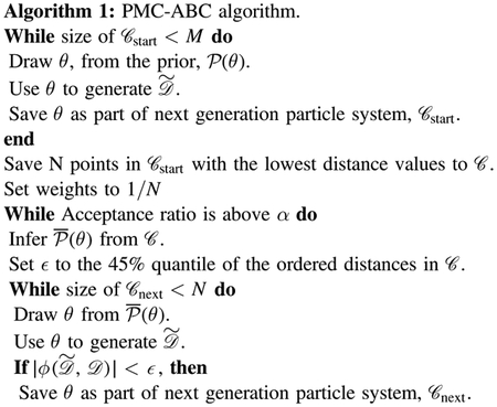
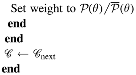
Appendix D
Ratio between M- and K-band Derived from Power-law and Log-normal Distributions
Any model that allows different flux-density PDFs for M-and K-band predicts a varying F(M)/F(K) ratio as a function of F(K ). This is true even when both distributions are power laws if the power-law index β differs for the two bands. A simple way to calculate the ratio function—that is, the ratio as a function of F(K)—is the assumption that the cumulative distribution functions (as defined in Equations (21) or (23)) are equal for all corresponding pairs [F(K ), (F(M)]. This is simply asking for a match of the lowest 5% in K-band with the lowest 5% in M-band, the lowest 10% with the lowest 10%, and so on. In other words, it assumes that when K-band rises, M-band rises, and when K-band falls, M-band falls. The simultaneous NIR (1.65–3.8 μm) light curves in the literature indeed demonstrate this behavior. Under this assumption, we get for Case 1 (power-law/power-law):
| (38) |
with F0,M, F0,K < 0. For Case 2 (power-law/log-normal),
| (39) |
with
| (40) |
and with F0,K < 0. For Case 3 (log-normal/log-normal),
| (41) |
In order to use the information about the flux-density ratio determined from the synchronous data , we can use this equation and extend the Equation (27) distance function to
| (42) |
with and w a chosen weight. (Here, w = 0.002 relative to the weights defined in Appendix B.2.)
The corresponding NIR spectral index
| (43) |
where AM and AK are the adopted interstellar extinctions in magnitudes. For our case with
| (44) |
and with λM = 4.5 μm and λK = 2.18 μm,
| (45) |
Appendix E
NIR Spectral Index as a Function of Flux Density
For synchrotron radiation from an electron energy distribution with an exponential cutoff, the spectrum in the optically thin frequency regime is a power-law with an exponential cutoff at a frequency ν0 (e.g., Bregman 1985). The flux density S(ν) at a given frequency ν in the optically thin regime is
| (46) |
with the spectral index of the optically thin power-law spectrum and k0 a proportionality constant. For typical electron energy cutoffs, ν0 will be located in or slightly above the NIR frequency range. Thus varying flux densities in the NIR and a flux-density-dependent NIR spectral index could be the consequence of a changing energy cutoff in the electron energy distribution.
We want to derive the flux-density dependence of the spectral index for this scenario. For a frequency (but still in the optically thin regime; i.e., in the submm regime close to 1 THz), Equation (46) becomes
| (47) |
and we can eliminate the proportionality factor:
| (48) |
This equation implies that while the flux density in the NIR overall scales with flux density in the submm, for a given submm flux density the NIR variability is caused by the changes in ν0. The flux-density ratio between two frequencies ν1 and ν2 is
| (49) |
and
| (50) |
Equation (48) gives
| (52) |
Inserting Equation (51) in Equation (50) gives
| (53) |
with
| (54) |
and
| (55) |
Footnotes
Supporting material: machine-readable table
The spectral index is defined here as .
The PDF of flux densities is the probability that an independent observation will yield a flux density in a particular interval.
The PSD is the Fourier transform of the autocorrelation function (e.g., Timmer & Koenig 1995, Equation (48)). In other words, the PSD measures how much the flux densities of two measurements separated in time are likely to differ, but the independent variable is spectral frequency—that is, 1/(time difference).
The terms “credible interval” and “credible limit” refer to intervals and their upper and lower limits that have a specified probability of containing the true value. In the Bayesian context, these intervals are directly derived from the posteriors.
Error bars include both statistical and estimated systematic uncertainties. The AM error bar is a corrected value from R. Schödel (2018, private communication).
ABC algorithms are routinely used in cosmology (see, e.g., Akeret et al. 2015).
In the variability literature as followed here, the definition of the structure function is such that a structure function of order M removes polynomials of order M − 1 from the data—that is, the first-order structure function is blind to DC offsets in the data. In the literature about turbulent media, V(τ) as defined here is called the second-order structure function.
It is not necessary to densely sample the shape of the structure function around the break timescale. Because the mock data are computed as the Fourier transform of the PSD, the break frequency contributes to all timescales. However, the plateau of the structure function at the longest timescales is directly related to the variance of the process and crucially helps constrain the PSD parameters.
Our C++ implementation (Appendix B) is based on FFTW, uses an efficient algorithm (Appendix C) for calculating structure functions, and is fully parallelized for large computational clusters.
This choice of parametrization was motivated by the reports that is invariant within uncertainties, at least over a wide range of timescales (except for very minor short-timescale fluctuations) and flux-density levels (Hornstein et al. 2007; Witzel 2014 but disputed by, e.g., Ponti et al. 2017). However, this parametrization permits a flux-density-dependent if βK≠ βM. In this case s loses its meaning as the M- to K-band ratio factor (see Appendix D).
When explaining results from Equation (7), we will use the variables ξ and η instead of their numerical values. With the uncertainties of ξ and η being strongly correlated, numerical values with uncertainties could be misinterpreted as independent.
References
- Akeret J, Refregier A, Amara A, Seehars S, & Hasner C 2015, JCAP, 8, 043 [Google Scholar]
- Astropym Collaboration, Robitaille TP, Tollerud EJ, et al. 2013, A&A, 558, A33 [Google Scholar]
- Baganoff FK, Bautz MW, Brandt WN, et al. 2001, Natur, 413, 45. [DOI] [PubMed] [Google Scholar]
- Balick B, & Brown RL 1974, ApJ, 194, 265 [Google Scholar]
- Bardeen JM, Press WH, & Teukolsky SA 1972, ApJ, 178, 347 [Google Scholar]
- Boehle A, Ghez AM, Schödel R, et al. 2016, ApJ, 830, 17 [Google Scholar]
- Bower GC, Markoff S, Dexter J, et al. 2015, ApJ, 802, 69 [Google Scholar]
- Bregman JN 1985, ApJ, 288, 32 [Google Scholar]
- Bremer M, Witzel G, Eckart A, et al. 2011, A&A, 532, A26 [Google Scholar]
- Cameron E, & Pettitt AN 2012, MNRAS, 425, 44 [Google Scholar]
- Capellupo DM, Haggard D, Choux N, et al. 2017, ApJ, 845, 35 [Google Scholar]
- Carpenter B, Gelman AD, Hoffman M, et al. 2017, JSS, 76, 1. [DOI] [PMC free article] [PubMed] [Google Scholar]
- Dexter J, Kelly B, Bower GC, et al. 2014, MNRAS, 442, 2797 [Google Scholar]
- Dibi S, Markoff S, Belmont R, et al. 2016, MNRAS, 461, 552 [Google Scholar]
- Diolaiti E, Bendinelli O, Bonaccini D, et al. 2000, Proc. SPIE, 4007, 879 [Google Scholar]
- Do T, Ghez AM, Morris MR, et al. 2009, ApJ, 691, 1021 [Google Scholar]
- Do T, Lu JR, Ghez AM, et al. 2013, ApJ, 764, 154 [Google Scholar]
- Dodds-Eden K, Gillessen S, Fritz TK, et al. 2011, ApJ, 728, 37 [Google Scholar]
- Dodds-Eden K, Porquet D, Trap G, et al. 2009, ApJ, 698, 676 [Google Scholar]
- Dodds-Eden K, Sharma P, Quataert E, et al. 2010, ApJ, 725, 450 [Google Scholar]
- Dolence JC, Gammie CF, Shiokawa H, & Noble SC 2012, ApJL, 746, L10 [Google Scholar]
- Drovandi CC, & Pettitt AN 2011, Biometrics, 67, 225. [DOI] [PubMed] [Google Scholar]
- Eckart A, Baganoff FK, Morris M, et al. 2004, A&A, 427, 1 [Google Scholar]
- Eckart A, Baganoff FK, Morris MR, et al. 2009, A&A, 500, 935 [Google Scholar]
- Eckart A, Baganoff FK, Schödel R, et al. 2006a, A&A, 450, 535 [Google Scholar]
- Eckart A, Baganoff FK, Zamaninasab M, et al. 2008a, A&A, 479, 625 [Google Scholar]
- Eckart A, García-Marín M, Vogel SN, et al. 2012, A&A, 537, A52 [Google Scholar]
- Eckart A, Schödel R, García-Marín M, et al. 2008b, A&A, 492, 337 [Google Scholar]
- Eckart A, Schödel R, Meyer L, et al. 2006b, A&A, 455, 1 [Google Scholar]
- Eisenhauer F, Genzel R, Alexander T, et al. 2005, ApJ, 628, 246 [Google Scholar]
- Emmanoulopoulos D, McHardy IM, & Uttley P 2010, MNRAS, 404, 931 [Google Scholar]
- Falcke H, Goss WM, Matsuo H, et al. 1998, ApJ, 499, 731 [Google Scholar]
- Falcke H, & Markoff S 2000, A&A, 362, 113 [Google Scholar]
- Fazio GG, Marrone D, Hora JL, et al. 2018, ApJ, in press [Google Scholar]
- Foreman-Mackey D 2016, JOSS, 1, 24 [Google Scholar]
- Frigo M, & Johnson SG 2005, Proc. IEEE, 93, 216 [Google Scholar]
- Gandhi P 2009, ApJL, 697, L167 [Google Scholar]
- García-Marín M, Eckart A, Weiss A, et al. 2011, ApJ, 738, 158 [Google Scholar]
- Genzel R, Schödel R, Ott T, et al. 2003, Natur, 425, 934. [DOI] [PubMed] [Google Scholar]
- Ghez AM, Hornstein SD, Lu JR, et al. 2005a, ApJ, 635, 1087 [Google Scholar]
- Ghez AM, Salim S, Hornstein SD, et al. 2005b, ApJ, 620, 744 [Google Scholar]
- Ghez AM, Wright SA, Matthews K, et al. 2004, ApJL, 601, L159 [Google Scholar]
- Gillessen S, Eisenhauer F, Quataert E, et al. 2006, ApJL, 640, L163 [Google Scholar]
- Guan X, Gammie CF, Simon JB, & Johnson BM 2009, ApJ, 694, 1010 [Google Scholar]
- Haubois X, Dodds-Eden K, Weiss A, et al. 2012, A&A, 540, A41 [Google Scholar]
- Herrnstein RM, Zhao J-H, Bower GC, & Goss WM 2004, AJ, 127, 3399. [DOI] [PubMed] [Google Scholar]
- Hora JL, Witzel G, Ashby MLN, et al. 2014, ApJ, 793, 120 [Google Scholar]
- Hornstein SD, Ghez AM, Tanner A, et al. 2002, ApJL, 577, L9 [Google Scholar]
- Hornstein SD, Matthews K, Ghez AM, et al. 2007, ApJ, 667, 900 [Google Scholar]
- Hughes PA, Aller HD, & Aller MF 1992, ApJ, 396, 469 [Google Scholar]
- Hunter JD 2007, CSE, 9, 90 [Google Scholar]
- Ishida EEO, Vitenti SDP, Penna-Lima M, et al. 2015, A&C, 13, 1 [Google Scholar]
- Jones E, Oliphant T, Peterson P, et al. 2001, SciPy: Open source scientific tools for Python, http://www.scipy.org/
- Karssen GD, Bursa M, Eckart A, et al. 2017, MNRAS, 472, 4422 [Google Scholar]
- Kelly BC, Bechtold J, & Siemiginowska A 2009, ApJ, 698, 895 [Google Scholar]
- Kelly BC, Treu T, Malkan M, Pancoast A, & Woo J-H 2013, ApJ, 779, 187 [Google Scholar]
- Kozłowski S 2016, ApJ, 826, 118 [Google Scholar]
- Krabbe A, Iserlohe C, Larkin JE, et al. 2006, ApJL, 642, L145 [Google Scholar]
- Kunneriath D, Witzel G, Eckart A, et al. 2010, A&A, 517, A46 [Google Scholar]
- Lenzen R, Hartung M, Brandner W, et al. 2003, Proc. SPIE, 4841, 944 [Google Scholar]
- Li J, Shen Z-Q, Miyazaki A, et al. 2009, ApJ, 700, 417 [Google Scholar]
- Mahadevan R 1998, Natur, 394, 651 [Google Scholar]
- Marjoram P, Molitor J, Plagnol V, & Tavaré S 2003, PNAS, 100, 15324. [DOI] [PMC free article] [PubMed] [Google Scholar]
- Marrone DP, Baganoff FK, Morris MR, et al. 2008, ApJ, 682, 373 [Google Scholar]
- Marrone DP, Moran JM, Zhao J-H, & Rao R 2006, ApJ, 640, 308 [Google Scholar]
- Marrone DP, Moran JM, Zhao J-H, & Rao R 2007, ApJL, 654, L57 [Google Scholar]
- Mauerhan JC, Morris M, Walter F, & Baganoff FK 2005, ApJL, 623, L25 [Google Scholar]
- McHardy IM, Koerding E, Knigge C, Uttley P, & Fender RP 2006, Natur, 444, 730. [DOI] [PubMed] [Google Scholar]
- Melia F, & Falcke H 2001, ARA&A, 39, 309 [Google Scholar]
- Meyer L, Do T, Ghez A, et al. 2008, ApJL, 688, L17 [Google Scholar]
- Meyer L, Do T, Ghez A, et al. 2009, ApJL, 694, L87 [Google Scholar]
- Meyer L, Eckart A, Schödel R, et al. 2006a, A&A, 460, 15 [Google Scholar]
- Meyer L, Schödel R, Eckart A, et al. 2006b, A&A, 458, L25 [Google Scholar]
- Meyer L, Schödel R, Eckart A, et al. 2007, A&A, 473, 707 [Google Scholar]
- Meyer L, Witzel G, Longstaff FA, & Ghez AM 2014, ApJ, 791, 24 [Google Scholar]
- Miyazaki A, Tsutsumi T, & Tsuboi M 2004, ApJL, 611, L97 [Google Scholar]
- Moffet AT 1975, in Strong Nonthermal Radio Emission from Galaxies, ed. Sandage A, Sandage M, & Kristian J (Chicago, IL: Univ. Chicago Press; ), 211 [Google Scholar]
- Morris MR, Meyer L, & Ghez AM 2012, RAA, 12, 995 [Google Scholar]
- Mossoux E, Grosso N, Bushouse H, et al. 2016, A&A, 589, A116 [Google Scholar]
- Neilsen J, Markoff S, Nowak MA, et al. 2015, ApJ, 799, 199 [Google Scholar]
- Neilsen J, Nowak MA, Gammie C, et al. 2013, ApJ, 774, 42 [Google Scholar]
- Nishiyama S, Tamura M, Hatano H, et al. 2009, ApJL, 702, L56 [Google Scholar]
- Özel F, Psaltis D, & Narayan R 2000, ApJ, 541, 234 [Google Scholar]
- Ponti G, George E, Scaringi S, et al. 2017, MNRAS, 468, 2447 [Google Scholar]
- Porquet D, Grosso N, Predehl P, et al. 2008, A&A, 488, 549 [Google Scholar]
- Rauch C, Ros E, Krichbaum TP, et al. 2016, A&A, 587, A37 [Google Scholar]
- Sabha N, Eckart A, Merritt D, et al. 2012, A&A, 545, A70 [Google Scholar]
- Sabha N, Witzel G, Eckart A, et al. 2010, A&A, 512, A2 [Google Scholar]
- Schödel R, Morris MR, Muzic K, et al. 2011, A&A, 532, A83 [Google Scholar]
- Schödel R, Najarro F, Muzic K, & Eckart A 2010, A&A, 511, A18 [Google Scholar]
- Shahzamanian B, Eckart A, Valencia SM, et al. 2015, A&A, 576, A20 [Google Scholar]
- Sharma P, Quataert E, Hammett GW, & Stone JM 2007, ApJ, 667, 714 [Google Scholar]
- Simonetti JH, Cordes JM, & Heeschen DS 1985, ApJ, 296, 46 [Google Scholar]
- Sisson SA, Fan Y, & Tanaka MM 2007, PNAS, 104, 1760. [DOI] [PMC free article] [PubMed] [Google Scholar]
- Subroweit M, García-Marín M, Eckart A, et al. 2017, A&A, 601, A80 [Google Scholar]
- Timmer J, & Koenig M 1995, A&A, 300, 707 [Google Scholar]
- Towns J, Cockerill T, Dahan M, et al. 2014, CSE, 16, 62 [Google Scholar]
- Trap G, Goldwurm A, Dodds-Eden K, et al. 2011, A&A, 528, A140 [Google Scholar]
- Trippe S, Paumard T, Ott T, et al. 2007, MNRAS, 375, 764 [Google Scholar]
- Uttley P, McHardy IM, & Vaughan S 2005, MNRAS, 359, 345 [Google Scholar]
- Witzel G 2014, AAS Meeting, 223, 238.04 [Google Scholar]
- Witzel G, Eckart A, Bremer M, et al. 2012, ApJS, 203, 18 [Google Scholar]
- Witzel G, Eckart A, Buchholz RM, et al. 2011, A&A, 525, A130 [Google Scholar]
- Witzel G, Lu JR, Ghez AM, et al. 2016, Proc. SPIE, 9909, 99091O [Google Scholar]
- Witzel G, Morris M, Ghez A, et al. 2014, in IAU Symp. 303, The Galactic Center: Feeding and Feedback in a Normal Galactic Nucleus, ed. Sjouwerman LO, Lang CC, & Ott J (Cambridge: Cambridge Univ. Press; ), 274 [Google Scholar]
- Yelda S, Lu JR, Ghez AM, et al. 2010, ApJ, 725, 331 [Google Scholar]
- Yuan F, & Bu D-F 2010, MNRAS, 408, 1051 [Google Scholar]
- Yuan F, Quataert E, & Narayan R 2003, ApJ, 598, 301 [Google Scholar]
- Yusef-Zadeh F, Bushouse H, Dowell CD, et al. 2006a, ApJ, 644, 198 [Google Scholar]
- Yusef-Zadeh F, Bushouse H, Wardle M, et al. 2009, ApJ, 706, 348 [Google Scholar]
- Yusef-Zadeh F, Roberts D, Wardle M, Heinke CO, & Bower GC 2006b, ApJ, 650, 189 [Google Scholar]
- Yusef-Zadeh F, Wardle M, Cotton WD, Heinke CO, & Roberts DA 2007, ApJL, 668, L47 [Google Scholar]
- Yusef-Zadeh F, Wardle M, Dodds-Eden K, et al. 2012, AJ, 144, 1 [Google Scholar]
- Yusef-Zadeh F, Wardle M, Heinke C, et al. 2008, ApJ, 682, 361 [Google Scholar]
- Yusef-Zadeh F, Wardle M, Miller-Jones JCA, et al. 2011, ApJ, 729, 44 [Google Scholar]
- Zamaninasab M, Eckart A, Witzel G, et al. 2010, A&A, 510, A3 [Google Scholar]
- Zhang S, Baganoff FK, Ponti G, et al. 2017, ApJ, 843, 96 [Google Scholar]
- Zhao J-H, Bower GC, & Goss WM 2001, ApJL, 547, L29 [Google Scholar]
- Zylka R, Mezger PG, & Lesch H 1992, A&A, 261, 119 [Google Scholar]
- Zylka R, Mezger PG, Ward-Thompson D, Duschl WJ, & Lesch H 1995, A&A, 297, 83 [Google Scholar]
Associated Data
This section collects any data citations, data availability statements, or supplementary materials included in this article.