Identifying statistically significant chromatin contacts from Hi-C data with FitHiC2

Abstract

Fit-Hi-C is a programming application to compute statistical confidence estimates for Hi-C contact maps to identify significant chromatin contacts. By fitting a monotonically non-increasing spline, Fit-Hi-C captures the relationship between genomic distance and contact probability without any parametric assumption. The spline fit together with the correction of contact probabilities with respect to bin- or locus-specific biases accounts for previously characterized covariates impacting Hi-C contact counts. Fit-Hi-C is best applied for the study of mid-range (e.g., 20 kb−2 Mb for human genome) intra-chromosomal contacts; however, with the latest reimplementation, named FitHiC2, it is possible to perform genome-wide analysis for high-resolution Hi-C data, including all intra-chromosomal distances and inter-chromosomal contacts. FitHiC2 also offers a merging filter module, which eliminates indirect/bystander interactions, leading to significant reduction in the number of reported contacts without sacrificing recovery of key loops such as those between convergent CTCF binding sites. Here, we describe how to apply the FitHiC2 protocol to three use cases: (i) 5-kb resolution Hi-C data of chromosome 5 from GM12878 (a human lymphoblastoid cell line), (ii) 40-kb resolution whole-genome Hi-C data from IMR90 (human lung fibroblast), and (iii) budding yeast whole-genome Hi-C data at a single restriction cut site (EcoRI) resolution. The procedure takes ~12 h with preprocessing when all use cases are run sequentially (~4 h when run parallel). With the recent improvements in its implementation, FitHiC2 (8 processors and 16 GB memory) is also scalable to genome-wide analysis of the highest resolution (1 kb) Hi-C data available to date (~48 h with 32 GB peak memory). FitHiC2 is available through Bioconda, GitHub and the Python Package Index.

Introduction

Analysis of chromosome conformation capture data

Powered by high-throughput DNA sequencing methods, chromatin conformation capture has enabled genome-wide analysis of the 3D folding of DNA within the eukaryotic cell nucleus^1–7. Specifically, the improvements in the efficiency, applicability and cost of Hi-C experiments have transformed our understanding of the principles governing domain-level organization of the genome as well as regulation of genes through distal enhancer elements⁸. Hi-C measures the pairwise contact frequency of genomic regions by a process that can be summarized as follows: crosslink, cut, label, religate, shear, enrich and sequence^4–7. Mapping, filtering and binning^9–11 of the millions or billions of paired-end reads that are sequenced from a Hi-C experiment provide rich information about genome-wide proximity between each possible pair of regions/bins (i.e., contact count) in a matrix format, which we refer to as contact maps here. However, the resulting raw contact counts heavily depend on the linear (i.e., one-dimensional) distance between interacting regions due to the random polymer looping effect and are confounded by technical biases of the Hi-C experiment and sequencing in general^12,13. A crucial computational task is to properly model all these known dependencies and biases, to tease apart the biologically meaningful and important interactions involving genes, gene regulatory elements and structural anchor points of the genome from Hi-C data. Our earlier method, Fit-Hi-C¹⁴, proposed a computational method to model the distance decay and account for technical biases, to find statistically significant intra-chromosomal Hi-C contacts. The protocol described here, named FitHiC2, extends Fit-Hi-C by incorporating various new computational modules and utilities (described below in detail) and an efficient reimplementation that allows FitHiC2 to scale for high-resolution Hi-C maps. This protocol walks through the steps necessary to run FitHiC2.

Improvements compared to the original Fit-Hi-C implementation

FitHiC2 is a significantly more powerful version of Fit-Hi-C. Chief among the changes is the introduction of new options and modules, performance enhancements, pre/post-processing utilities and an easily installable command line version of the tool. More specifically:

• (i)The re-implementation described here allows the tool to run on the highest-resolution Hi-C datasets currently available (1 and 5 kb) while retaining the same statistical significance estimation procedure as our previous version. These improvements were made possible by significantly refactoring the code and developing more efficient data structures to hold possible interactions at higher resolutions, especially when the user specifies that the Hi-C data will be analyzed at fixed-size genomic bins, which is a widely used practice in the analysis of Hi-C data. This is a substantial improvement because the previous version would not scale to such high-resolution maps due to memory usage.
• (ii)Another important change is the addition of new options such as ‘-x’, which allows the user to analyze different portions of their dataset such as inter-chromosomal-only, intra-chromosomal-only or all interactions. The recommended settings for each option are described in detail in the Procedure and in Table 1, and options that were added only in FitHiC2 are marked with an asterisk.
• (iii)We also introduce a new module named ‘merging filter’ that we recently used for HiChIP data analysis¹⁵, which helps eliminate indirect/bystander interactions happening around direct contacts between loop anchors. For high-resolution and deeply sequenced Hi-C maps, this module allows elimination of a significant portion of reported contacts without sacrificing recovery of key loops such as those between convergent CTCF binding sites.
• (iv)Further, we developed a number of utilities to aid analysis both before and after FitHiC2 is run. These utilities span use cases from generating the input files from commonly used Hi-C data formats, to visualizing and exploring a hypertext markup language (HTML) summary of the results as well as scripts to convert FitHiC2 output to formats accepted by commonly used browsers such as the WashU Epigenome Browser (http://epigenomegateway.wustl.edu) and the UCSC Genome Browser (http://genome.ucsc.edu).
• (v)Finally, FitHiC2 is now easily installable on the command line through the Bioconda distribution platform or through the Python Package Index.

Table 1 |.

Description and flag of each of FitHiC2’s options Options

Option flag	Description of option
—help, -h	Displays help message of all available options
—interactions, -i	Path to the interactions file being used. This flag is required.
—fragments, -f	Path to the fragments file being used. This flag is required.
—outdir, -o	Path to a directory where all the output files will be written. If the directory is not already made, FitHiC2 will automatically create it. This flag is required.
—resolution, -r (*)	Resolution of dataset being used. If the dataset is not fixed size, then a value of 0 should be used here. This flag is required.
—biases, -t	Path to the bias file being used. This flag is highly recommended.
—passes, -p	Number of spline passes. If no refinement to the null model is desired, then provide 1. The default value is 1.
—noOfBins, -b	Number of equal occupancy bins into which the locus pairs within the specified genomic distance range are divided. This parameter does not have a significant impact on the spline fit in general. We suggest using 100 or 200 in most cases.
—mappabilityThres, -m	This is the minimum coverage necessary to call a locus mappable and include it in the calculations. The default value of 1 could also be used as a binary filter if the input file has 1 for mappable and 0 for unmappable regions. Higher values may be desired if the data is of high sequencing depth and input files correctly reflect the coverage for each locus.
—lib, -l	The library name being utilized. This changes the name of the prefix appended to the outputs of FitHiC2. This value has no effect on actual analysis, and its default is fithic.
-distUpThres, -U	This value determines the upper bound of interaction distances to be considered.
—distLowThres, -L	This value determines the lower bound of interaction distances to be considered.
—biasUpperBound, -tU (*)	This value determines the upper bound above which a locus and all contacts involving the locus will be discarded. The default value is 2.
—biasLowerBound, -tL. (*)	This value determines the lower bound below which a locus and all contacts involving the locus will be discarded. The default value is 0.5.
—visual, -v	Visual option if graphs would like to be outputted. These will be outputted in the same directory as specified in -o.
—contactType, -x. (*)	Option to determine which interactions would be studied. The options are interOnly, intraOnly and All. The default value is intraOnly (intra-chromosomal interactions).
—version, -V	Version number is outputted, and FitHiC2 exits.

^*Option is exclusive to FitHiC2.

The purpose of this protocol is to walk users, old and new, through a series of representative use cases to aid in their own analyses conducted with this new version of Fit-Hi-C named FitHiC2.

Overview and development of the method

FitHiC2 is a programming application designed to compute statistical confidence estimates to Hi-C contact counts by jointly modeling the random polymer looping effect and potential technical biases in Hi-C data sets¹⁴. FitHiC2 first learns an empirical null using observed contact counts to model the expected contact count or contact probability conditioned on the genomic distance between interacting regions. This is achieved by first using an equal occupancy binning strategy that divides the total number of contact counts (N, i.e., sum of the Hi-C matrix entries) between all locus pairs in range (M pairs) into a user-specified number of bins (b bins), each with approximately equal number of contacts (~N/b). Such binning is achieved by sorting all locus pairs with a non-zero contact count with respect to increasing genomic distance between the two ends of the pair and breaking this sorted list into b bins, where the first bin has all the pairs with the smallest genomic distances whose total contact count is at least N/b. FitHiC2 employs tiebreak conditions to avoid assigning two pairs with the same genomic distance into two different bins, and, hence, the total contact count per bin may show a slight deviation from the desired bin total of N/b. For each such bin, we then compute the average genomic distance (x-axis) and contact probability (y-axis) among all pairs (including possible pairs with zero contact counts) in that bin. FitHiC2 then fits a cubic smoothing spline (third degree polynomial) to these x, y values (one per bin) to learn a continuous function that relates these two entities. Equal occupancy binning, instead of fixed-size bins with respect to genomic distance intervals, prevents having high variance bins such as bins for long genomic distances with only a small number of contact counts, whereas the smoothing spline fit allows contact probability to be defined (i.e., exact look up from the spline function) for each possible genomic distance. FitHiC2 also allows for the refinement of the initial spline fit by removing ‘positive outliers’ that correspond to bona fide (i.e., non-null) interactions and refitting the spline to the remaining interactions that belong to the random (i.e., null) portion of the data.

Another feature of FitHiC2 is that it corrects expected contact probabilities learned from the spline fit described above through integrating normalization factors (i.e., bias values), which are computed per locus/bin by matrix balancing–based Hi-C normalization methods such as iterative correction and eigenvector decomposition (ICE)¹² or Knight and Ruiz (KR)^4,16. Using the corrected contact probability and the observed contact count for each entry in the raw contact map, FitHiC2 computes a binomial P value for the significance of observing a contact count that is at least equal to the observed integer count value or higher. All P values are then subjected to multiple testing correction using the Benjamini-Hochberg procedure to gather Q values, which represent the minimum false discovery rate (FDR) threshold at which the contact is deemed significant¹⁷. Overall, FitHiC2 computes accurate empirical null models of contact probability without any distribution assumption, uses these probabilities for calculation of a binomial P value; successfully corrects for binning artifacts, distance dependence and technical biases; and provides biologically relevant statistical confidence estimates that capture known interactions¹⁴.

Step-by-step workflow of FitHiC2

The procedure described here outlines the complete workflow starting from generation of FitHiC2 input files to final analysis and visualization of the statistical confidence estimates computed (Fig. 1). This procedure assumes that the user has used an existing tool to align and filter the sequencing data from a Hi-C assay. Through several utility functions, the FitHiC2 package allows multiple possible input formats and entry points to the overall pipeline (Fig. 1). FitHiC2 first reads the nonzero interaction counts within the user-specified range and builds an index of genomic distances and their associated contact counts. These contact counts are placed into equal occupancy bins, and the associated genomic range of each bin is recorded. Next, FitHiC2 utilizes the fragments file to either enumerate all possible fragment pairs (in the case of non-fixed-size data) or loop through the possible fragment pairs (in the case of fixed-size data) to compute for each equal occupancy bin the number of all possible fragment pairs that fall within the bin’s distance interval and in turn, the average contact count and average distance of all pairs within that specific bin. FitHiC2 then reads and stores the estimated bias value for each fragment/locus if a bias values file is inputted (not required but very strongly suggested). Finally, the null model of a univariate cubic spline function is fit to the average distance versus the average contact count for each bin, and the resulting spline is subjected to antitonic regression to ensure that it is non-increasing with respect to increasing distance.

Fig. 1 |. FitHiC2 flowchart.

a, A brief overview of the main stages of analysis performed by FitHiC2. b, A more complete overview of all scripts and utilities incorporated into the FitHiC2 repository. FitHiC2 provides multiple different entry points to the workflow (denoted by i1 and i2), thereby allowing several file formats to be converted to expected input files, namely, contact counts, fragments and bias values files. For b, the numbers listed in boxes represent the corresponding steps in the Procedure section.

Once the spline is fit, the P value calculation consists of reading each entry (i.e., a pair of loci with a non-zero contact count) from the contact count file, computing the prior contact probability of this locus pair using their genomic distance by a lookup from the spline fit, multiplying that prior probability by the bias value for each locus and plugging that corrected probability P into a binomial distribution, where n is the observed total sum of contact counts, and k is the observed contact count for that given interaction (see Fig. 1 of Ay et al.¹⁴). After correcting for multiple testing, these P values and their corresponding Q values are appended to the entry/line read from the contact counts file and outputted to a significance file. If the user specifies through the ‘number of passes’ parameter, additional passes of spline fit will be performed on the refined null models. At each pass, positive outliers will be filtered using a stringent P value threshold of 1/M, where M is the total number of locus pairs, to refine the null. Such outliers are removed from observed as well as from possible pairs of loci during spline fit; however, they will be considered again and assigned confidence estimates alongside non-outliers. Our recommendations with respect to this step are discussed in detail in the Procedure section.

Applications of the method

FitHiC2 may easily be applied to the study of intra-chromosomal, inter-chromosomal, and whole genome interactions and is perfectly suited to complement any and all Hi-C analysis pipelines. Our Google Group (https://groups.google.com/forum/#!forum/fithic) provides a community for users and allows the free exchange of knowledge and ideas. In addition, the tool is freely available and easily installable through GitHub and the Python Package Index.

An important aspect of FitHiC2 is that it does not make any assumptions about the size or the structure of the genome besides expecting that the contact probability will not increase with increasing genomic distance on average. It also does not require a strict minimal sequencing depth or a minimum or maximum resolution for contact maps. These features allowing FitHiC2 to be very flexible are mainly due to our use of an empirical null model that adjusts to the input data. Even though used mostly for human and mouse Hi-C data, FitHiC2 has found use in studies of a wide range of organisms, including yeasts, malaria parasites and plants including cotton and Arabidopsis thaliana^18–22.

While FitHiC2 may be applied in many different settings where statistical confidence estimates of chromosomal interactions are of interest, we suggest that it be used to interrogate only the range and type of interactions that are of biological relevance and are reasonable to study with the sequencing depth and resolution at hand. More specifically, it may make sense to study all inter- and intra-chromosomal interactions for a small genome (e.g., yeast) at a moderate bin size (e.g., 5 or 10 kb) or for a large genome with big window sizes (e.g., human genome at 40 or 100 kb). Such an analysis may reveal preferences of large genomic regions on different chromosomes to colocalize with each other. However, it will not be as appropriate to analyze all inter- and intra-chromosomal interactions with no distance limit for the human or mouse genome at 5- or 1-kb resolution without sufficient sequencing depth. Moreover, by interrogating a very large distance range and including inter-chromosomal interactions, say at 5-kb resolution, the statistical power of detecting significant interactions at more relevant ranges, say up to 2 Mb, will be hampered due to a very heavy multiple-testing burden. Regardless, we provide options and parameter settings that allow users to study any subset or all interactions as they desire.

We also designed FitHiC2 to have versatile, human-readable inputs (Boxes 1–4) to enable users to select from a wide array of Hi-C analysis tools, which can then feed into our workflow. One such tool, HiCPro¹⁰, is commonly used and provides a conversion script between their output and FitHiC2’s input format. Such conversion of file formats is also described in our Procedure. HiCPro already provides a script for Hi-C normalization using ICE. However, the normalization procedure, unlike the steps of mapping, filtering and contact map generation, is not included by default in most of the existing Hi-C data-processing tools. In view of this, we also developed HiCKRy, a Python implementation of the KR algorithm for matrix balancing¹⁶, and bundled it with our release of FitHiC2. Regardless of which algorithm is used to normalize Hi-C data (ICE, KR, etc.), integration of per-locus bias values from the normalization to FitHiC2 is critical for reducing the number of false positives and can be accomplished through creating a very simple file, the format of which is described in Box 3.

Box 1 |. validPairs file format

The validPairs file is produced by most Hi-C assay analysis pipelines such as HiCPro¹¹ and Juicer³⁷; although its exact name and format may vary from tool to tool, the essential set of fields is mostly present. This file is the result of mapping fastq files for each read end to the reference genome and joining them using the read identifiers to get a set of paired-end reads with both ends mapped to unique locations. Depending on the pipeline, this set may or may not contain chimeric read ends that are mapped only after a second round of read mapping. This file could also be filtered using stringent mapping quality criteria (MAPQ >30) and/or from unwanted chromosomes or contigs. Typically, the first column corresponds to a read identifier pertaining to the fastq read, the next six columns refer to the chromosome, coordinate and strand where the first read end and the second read end of the paired-end read mapped, respectively. The last column refers to the total distance of read mapping coordinates to the nearest restriction enzyme cut site location for each end. FitHiC2’s provided script requires only chromosome identifiers and mapping coordinates (columns 2, 3, 5 and 6) while converting the valid pairs file to contact maps. Therefore, any file with the relevant chromosome and coordinate information located in those columns (maintaining the expected ordering of columns) will be successfully converted to a contact counts file to be used as the input of FitHiC2 (Boxes 1–4).

validPairs file format

Identifier 1	chr2	147501087	+	chr7	120502771	–	180
Identifier 2	chr8	95345354	+	chr13	72476846	+	296
Identifier 3	chr11	8481536	+	chr11	8527887	–	455

Box 4 |. FitHiC2 compatibility with other tools

HiCPro

FitHiC2 also provides a utility to automatically generate its input files directly from the output of a commonly used Hi-C mapping tool, HiCPro. This conversion script is provided within utilities as well as by HiCPro under their bin/utils/hicpro2fithic.py. This script uses HiCPro’s bed and matrix files simultaneously to generate the input files for FitHiC2 as described in Box 2. In addition, the bias files generated through HiCPro’s ICE normalization method (for HiCPro version 2.10 or newer) can also be inputted and formatted, alongside other files, to FitHiC2’s input bias file format described in Box 3.

.hic Files

If the Juicer platform was previously used for analysis, the resulting .hic files may be used in conjunction with FitHiC2 through the development of another utility developed. The script titled ‘createFitHiCContacts-hic.sh’ uses four arguments. The first is the text file output by the juicebox dump command, and the next two arguments are the two chromosomes to which the text file corresponds. The last argument is the name of the output file to write the resulting interaction counts.

Box 3 |. FitHiC2 bias file format

As mentioned above and in the literature, it is critical to properly normalize Hi-C data for potential technical biases. It is also crucial for FitHiC2 to correct for these normalization factors, which are called bias values, in its significance estimation to avoid false positives. Many Hi-C data-processing pipelines already provide means to normalize Hi-C data and gather these biases. We also provide our own Python implementation of the KR algorithm (HiCKRy), which was first used for Hi-C data by Rao et al.⁴, for users to carry out normalization and compute bias values within FitHiC2 package.

Regardless of the normalization platform, the output bias file should have the first two columns denote bin identifiers that are used in the contact counts file, which are generally the chromosome and the midpoint of each bin. The third column corresponds to the actual bias value generated by the normalization method. A value of −1 in the third column means that this column was skipped in the normalization step and that contact count entries involving this locus will be removed from consideration during FitHiC2. The bias values (excluding −1s) should be centered on 1, with the expectation that a value of 1 represents no bias, a value <1 represents that this region is underrepresented in contact counts (i.e., lower number of total contact counts than average) and vice versa for a value >1.

Bias file format

chr1	60000	−1
chr1	100000	0.146
chr1	140000	1.023

In addition, FitHiC2 provides users with an output (Box 5) that can easily be converted into formats for a variety of other tools together with an HTML report (Box 6). The Procedure walks the user through how to convert FitHiC2 output into an input for the WashU Epigenome Browser or the UCSC Genome Browser; an example of each is reproduced in Box 7.

Box 5 |. FitHiC2 output files

FitHiC2 produces two important files for every spline fit conducted. The first file is the ‘$libraryname.fithic_pass $i’ file, where library name is the user specified ‘−1’ flag, and i refers to the ith spline fit. This file consists of five total columns depicting the bin statistics used by this run of FitHiC2, an example of which is reproduced below:

Average genomic distance	Contact probability	Standard error	No. of locus pairs	Total contact counts
120,000	6.96 × 10−07	0.00	77,331	3,667,637
160,000	5.90 × 10−07	0.00	77,307	3,107,143

This file depicts how each bin was created and the various statistics FitHiC2 used to compute the spline. In addition to the visual graphs, this is a key file to study if one is unsure of the results.

The second file is the ‘$libraryname.spline_pass’ file. This file is a 10-column file. The first five columns will be exact copies of the columns within the contact maps file. An example of the next five columns is provided below:

P value	Q value	Bias1	Bias2	Expected contact count
1.00	1.00	–1	–1	12.87
1.0337 × 10−07	5.7828 × 10−07	0.8124	0.7742	32.21

The P value and Q value are the statistical significance of the interaction depicted in that row as determined by FitHiC2. The next two columns list the bias values for each respective genetic locus, which are ‘–1’ for loci that were excluded from normalization or had bias values out of the desired range specified either by default [0.5, 2] or by the user through —biasLowerBound and —biasUpperBound options. The last column reports the expected contact count for the specific locus pair, which is calculated by multiplying the prior probability by the sum of all contact counts within the specified distance range, which is then multiplied with both bias1 and bias2 values.

Box 6 |. FitHiC2 HTML output

FitHiC2 provides a script to convert the output of the -v, visual option, into an HTML report for easy viewing and analysis. The exact usage of the script is described in the Procedure and is flexible to however many spline passes the user ran. The HTML report includes links to log file, the statistical significance estimates and the bin statistics outputted by FitHiC2. In addition, the graphs FitHiC2 created will be embedded into the HTML report, allowing easy transfer of files.

Box 7 |. Visualizing FitHiC2 output in genome browsers

The set of significant interactions reported by FitHiC2, as well as the input Hi-C contact maps, can be visualized on multiple different platforms, most of which have been discussed in a recent review³⁸. In this Procedure, we demonstrate how to format FitHiC2output for visualization on one such platform, namely the WashU Epigenome Browser (Steps 14–21). Additionally, we have created a simple script (visualize-UCSC.sh) to convert the output of FitHiC2 into a visualization input for the UCSC Genome Browser. For the sake of brevity, we do not describe the usage in this Protocol; however, instructions can be found in the README for FitHiC2. The example regions below show arcs, which correspond to significant interactions computed by FitHiC2 at a −log10(Q value) threshold of 10 for a select region of the Rao GM12878 5-kb chromosome 5 data analyzed in the protocol. a, Snapshot of this interaction in the UCSC Genome Browser. b, Snapshot of this interaction in the WashU Epigenome Browser.

Related methods

In recent years, a number of computational methods have been developed, which aim to identify significant interactions from and/or assign confidence estimates to Hi-C contact maps. Since a detailed description and full comparison of these different methods is beyond the scope of this protocol, we refer the readers to recent review articles that outline features of each tool and discuss their advantages and disadvantages with respect to each other^9,10,23. Several such tools depend on epigenomics data other than Hi-C to prioritize a subset of (e.g., promoter-enhancer) Hi-C interactions²⁴, whereas others are primarily for comparison of Hi-C data from two different conditions²⁵. The tools that are more directly comparable to Fit-Hi-C/FitHiC2 include HiCCUPS⁴, HOMER (http://homer.ucsd.edu/homer/), GOTHiC²⁶ and the more recent HiC-DC²⁷. All of these tools, including FitHiC2, are designed to analyze standalone Hi-C contact maps, but they significantly differ from one another in their background estimation and distribution assumptions.

FitHiC2 computes the expected number of contacts (or contact probability) from a global background that considers all possible pairs of bins in the desired distance range or the specified interaction type. It then corrects the contact probability from the global expectation represented by a spline for technical biases computed on a per-bin basis prior to calculation of the binomial P value. GOTHiC, a later method, simply drops the modeling of the change in contact probability with respect to genomic distance (i.e., the spline-fitting of FitHiC2) and computes a binomial P value for a given pair of bins using the observed count, coverage of each bin and the total number of reads in the experiment. As a result, GOTHiC confidence estimates report most of the very-short-range genomic bins as significantly interacting, which leads to very low specificity of interaction calling²³. The HOMER Hi-C workflow, as part of the overall HOMER suite, also provides a statistical test for comparing the observed contact counts to an expected count. Akin to GOTHiC, HOMER uses coverages of each bin in calculation of the expected count for that bin pair; however, it also considers the scaling of counts with respect to genomic distance, unlike GOTHiC and similar to FitHiC2. HOMER’s distance scaling model simply takes an average at each possible genomic distance (only possible with fixed-size bins) and does not enforce monotonicity or account for the high variance of contact counts for pairs at large genomic distances. Similar to GOTHiC and FitHiC2, HOMER also plugs in the observed counts to the binomial distribution for computing P values.

Two methods that diverge from the use of binomial P values are HiCCUPS and HiC-DC. HiCCUPS employs a set of heuristics to quantify local enrichment of a contact count cluster (i.e., several adjacent entries in the contact map) with respect to its neighboring pixels and couples this quantification with several criteria to report only the centroid if a cluster is deemed significantly enriched with respect to all criteria⁴. The use of local background and the reporting of only the centroid of a cluster leads to identification of only a small set of interactions as significant. The resulting set of interactions mainly corresponds to strong loops between CTCF-bound boundaries of topological domains and/or loop domains^4,28. Even though these structural interactions are of utmost importance in understanding the domain level of genome organization, because of its high stringency and requirement for deeply sequenced Hi-C data, HiCCUPS lacks the sensitivity to capture many of the functionally important within-domain interactions that link regulatory elements such as enhancers and promoters to each other. A more recent method, HiC-DC, borrows several elements from Fit-HiC (e.g., spline fit and null refinement) and couples them with a zero-truncated negative binomial regression (i.e., hurdle regression) model, which accounts for inflation of zeros and overdispersion of contact counts in Hi-C data. Overlap analysis of HiC-DC and Fit-Hi-C calls reveals a significant amount of overlap for long-range contacts (>500 kb), but the overlap was much lower for contacts with shorter distances²⁷. Overall, however, the lack of an orthogonal set of genome-wide chromatin contacts (i.e., not from conformation capture) that could be regarded as a gold standard makes it difficult to assess the biological relevance of the set of interactions reported by each one of these methods.

Assessment of FitHiC2 interaction calls

Since the original Fit-Hi-C manuscript included several analyses for evaluation of the biological relevance of identified interactions¹⁴, in this protocol, we focus on evaluation of the newly added features in FitHiC2, which are the introduction of the merging filter (Box 8) and inclusion of inter-chromosomal interactions as an option. As described here for Hi-C and in our recent work for HiChIP data¹⁵, the merging filter step retains the strongest interactions that are also mutually distant by a number of bins (W) in at least one of the interacting ends. That is, if both endpoints of two interactions are within W bins, one of the interactions would not be reported after the merging filter. First, to decide the value of W empirically, we have tested FitHiC2 with three different values of W (W = 2, 5 or 10) in terms of its recovery performance for an extensively studied small set of interaction calls from HiCCUPS with or without considering convergent CTCF binding for the GM12878 in situ Hi-C data⁴ (Fig. 2a). Since W = 2 achieves a higher overall recovery compared to 5 and 10 and shows an equal performance to the full set of FitHiC2 interaction calls without merging with less than one-third of the interaction calls, we select W = 2 as our default option. Note that the optimal setting may be different for data with different resolutions and sequencing depth. In another evaluation of the merging filter (M), we show that both the reduction in interaction calls reported and the preservation of HiCCUPS recovery are reproducible between the two replicates of GM12878 Hi-C data for FitHiC2 (Fig. 2b). We observe similar results when we consider HICCUPS calls that overlap for a pair of convergent CTCF binding motifs as our reference (3,307 out of 8,519) (Fig. 2c).

Box 8 |. FitHiC2 interaction filtering

In FitHiC2, we have developed a post-processing method for distinguishing direct interactions from enrichments of contacts among their neighboring loci, which can be explained away by such direct interactions¹⁵. This method (merging filter) works first by merging neighboring loop calls into one connected component in the binary interaction matrix (0 = not significant, 1 = significant) and then by iteratively picking the strongest loop/interaction (FitHiC2 Q value) that is not within a defined vicinity of any of the readily picked loops in the result set to be reported after filtering. The vicinity between two loops is defined by a threshold of distance in terms of number of bins (default is 2) for each end of the loop simultaneously (i.e., left end of loop1 within ± two bins of the left end of loop2, and the same holds for the right end). This merging filter step significantly decreases the number of significant interactions and is useful to decrease the search space of interesting Hi-C calls. Three scripts perform this action: two are bash scripts that merge and filter the interactions for the user, and one is a Python script with more user options. For most users, the unparalleled bash script will be sufficient. An example of its usage is described in the Procedure. All three are described in detail in the FitHiC2 documentation. We have provided detailed evaluation of the merging filter in Fig. 2.

Fig. 2 |. Reproducibility and validation of FitHiC2 calls.

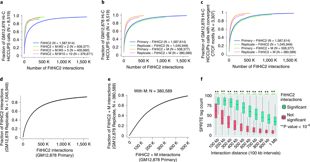
We use whole-genome 5-kb GM12878 data from Rao et al.⁴ with two replicates (‘Primary’ and ‘Replicate’). We consider the distance range of 15 kb to 1 Mb for all interaction calls and use 5-kb resolution contact maps to identify significant interactions at an FDR of 0.01 for FitHiC2 for each figure. a, The recovery of HiCCUPS calls from GM12878 Hi-C data using different window sizes for the merging filter in FitHiC2 on the Primary replicate Hi-C data. The fraction of reference interactions (HiCCUPS calls in this case) recovered by FitHiC2 calls when taking the top-k (x-axis) number of significant interactions sorted according to decreasing significance. b, Similar to a but when W = 2 is used for both the Primary and the Replicate sample. c, Same as b but when only the HiCCUPs calls with convergent CTCF motifs (3,307 out of 8,519 total) are used as the reference set. d, Reproducibility of FitHiC2 interaction calls between the two replicates of GM12878 Hi-C data. e, Same as d but when the merging filter is employed. f, Enrichment of SPRITE tag counts (10-kb binned GM12878 SPRITE data³) of FitHiC2 significant interactions from GM12878 5-kb resolution Hi-C data.

In terms of the overlap of interaction calls between the two replicates, the merging filter leads to a slight decrease compared to no filter (from ~93% to ~79% with overlap computed using 5-kb slack¹⁵) when we consider the percentage of interaction calls from the second replicate that are recovered by that of the primary replicate (Fig. 2d and e). The concave shape of these recovery plots also suggests that the more stringent set of calls in one replicate is likely to have an overlapping call in the other compared to less stringent ones, highlighting the consistency of ranking among significant calls by FitHiC2 between the replicates regardless of the use of the merging filter. When we consider the overlap of FitHiC2 calls on the same Hi-C data that is binned at different resolutions (1- and 5-kb binned primary replicate GM12878 data), we observe that even though the number of resulting calls varies quite significantly, 96% of the interactions reported at 1-kb resolution (19,164 out of 20,050) overlap with a significant interaction at 5-kb resolution.

Given the large number of interactions reported by FitHiC2 at 5 kb but not by HiCCUPS, we next investigate the biological relevance of FitHiC2-specific calls. We identify an additional 10,938 interactions with convergent CTCF binding with FitHiC2 from the primary GM12878 replicate, which were not in the set of 3,307 reported by HiCCUPS. Furthermore, when compared against a set of predictions of promoter-enhancer interactions using a recently proposed activity-by-contact model²⁹, for GM12878 FitHiC2 with a merging filter captured 13,502 out of 17,023 contacts, whereas HiCCUPS loops covered only 1,667 for the distance range of 15 kb–1 Mb. These results suggest that at least a subset of the additional interactions reported by FitHiC2 is likely functional either by contributing to domain- and sub-domain-level organization of the chromatin or by bringing distal enhancers in close proximity to their potential target genes.

To further evaluate FitHiC2 interaction calls, we ask whether they are in agreement with contact information from a recent crosslink-free assay named Split-Pool Recognition of Interactions by Tag Extension (SPRITE)³ to capture chromatin conformation. Comparing FitHiC2 interaction calls for GM12878 Hi-C data at 5-kb resolution stratified into 10 distance ranges (0–100 kb, 100–200 kb, etc.) with 10-kb binned GM12878 SPRITE data, we show that pairs of regions with FitHiC2 called interactions are significantly enriched in SPRITE tag counts at each distance range compared to pairs with no significant FitHiC2 interaction (Fig. 2f). This suggests that FitHiC2 calls from Hi-C data are supported by an orthogonal method that does not depend on crosslinking of chromatin.

Finally, we focus on the inter-chromosomal interaction calls from FitHiC2 in terms of their reproducibility across replicates and their overlap with previously identified inter-chromosomal translocations, which by definition create very strong and ‘significant’ interaction enrichments by adjoining regions from two different chromosomes. When we apply FitHiC2 in the ‘-x interOnly’ mode to a subset of chromosomes (chr10–15) for two replicates of the GM12878 Hi-C data at 100-kb resolution, we identify 8,573 and 1,887 significant interactions from the primary and secondary replicates, respectively. Nearly half of the interactions from the secondary replicate are also reported in the first when we consider an exact overlap. This percentage goes up to 78% when we allow a one-bin slack (i.e., 100 kb) for overlap calculation. To assess the overlap of FitHiC2 inter-chromosomal interactions with previously predicted translocations in cancer cells^30,31, we use Hi-C data at 40-kb resolution from CAKI2 (renal carcinoma) and T47D (breast cancer) cell lines³¹. For CAKI2, 4,034 out of 6,208 significant inter-chromosomal interactions (1% FDR) fall on the 20 pairs of chromosomes (out of 253 possible chromosome pairs) with translocations. Over 80% of these interactions lie within 1 Mb of a translocation call from HiCtrans³⁰. Similarly, for the T47D cell line, 950 out of 2,325 inter-chromosomal calls are from 16 different translocated chromosome pairs with 907 (>95%) within 1 Mb of a HiCtrans call. These results suggest that an important fraction of inter-chromosomal ‘interactions’ may actually indicate chromosomal rearrangements. Note that, unlike intra-chromosomal interactions where we use all possible pairs among the regions passing an initial filter (including those with zero counts) in the computation of prior contact probability, for inter-chromosomal interactions, we omit the pairs with no count from the probability calculation due to an extremely large number of zeros (>97%).

Limitations

The limitations of FitHiC2 currently include the technical requirements necessary to run FitHiC2 and the domain knowledge required to determine appropriate parameters and settings for each data set. These parameters include selection of a contact map resolution and a genomic distance range to consider. Another critical limitation relates to misunderstanding or incomplete understanding of the documentation in terms of how normalization is taken into account in FitHiC2. This has to be achieved through using the bias file together with raw (integer) contact counts and not the normalized counts. Under no circumstances does FitHiC2 expect normalized counts as an input or should it be used with normalized counts directly. The wrong parameters, settings or input files have the potential to severely impact the quality of downstream analysis, potentially leading to many false positives as well as false negatives in some cases.

Another important limitation of FitHiC2 that is also an intended feature is the dependency of significance estimates and the number of significant contacts on the read depth of the Hi-C library. This behavior is similar to peak calling methods of other genomics/epigenomics data such as ChIP-seq and allows full utilization of the high sequencing depth when available. Given that Hi-C contact maps are generally far away from saturation, we believe that the ability to report more discoveries with increased sequencing depth is a desired feature. However, this may complicate analysis when FitHiC2 estimates from two or more Hi-C contact maps with different sequencing depths are directly compared with each other. One trivial solution to this would be downsampling before FitHiC2 for comparative studies. Another possibility would be to use a certain number of strongest contacts (i.e., top-k with lowest P value) instead of a fixed Q value threshold.

Experimental design

The Procedure outlined in this protocol will follow applying FitHiC2 to study three representative use cases and assign statistical confidence estimates for each dataset: (i) fixed-size chromosome 5 Hi-C data at 5-kb resolution of an IMR90 cell line⁴, (ii) restriction fragment resolution Hi-C dataset from budding yeast⁵ and (iii) fixed-size whole-genome data at 40-kb resolution of an IMR90 cell line^28,32. We recommend that users not familiar with Hi-C data first follow along using these test datasets before applying FitHiC2 on their own datasets. FitHiC2 requires the contact maps file and the fragment mappability file in the format described in Box 2; however, the Procedure will describe how to generate these files using commonly produced files from a host of other Hi-C tools.

Box 2 |. FitHiC2 required input file format

FitHiC2 takes two required input files even though it is highly suggested that a third one, the bias file, is also used for correcting potential technical biases. The first required file is the contact counts file in the sparse format, listing each pair of bins with a nonzero count observed from the Hi-C data. FitHiC2’s interaction counts file is formatted with the first two columns representing the chromosome identifier (name or number) and the midpoint of one interacting genomic region and the next two columns representing the same for the second region. The fifth column corresponds to the contact count between these two chromosomal regions. This file must be compressed (using gzip) in order to be read by FitHiC2. The exact format is described below and may be checked with the command (zcat FILE | head).

Contact counts file format

chr1	20000	chr10	135340000	1
chr1	20000	chr10	26380000	1
chr1	20000	chr11	19180000	3

The second required input is the fragments file, listing every possible genomic bin in the genome that could appear in the contact counts file. An example of this file is shown below. The first column and the third column must denote bin identifiers that are used in the contact counts file, which are generally the chromosome and the midpoint of each bin. The second column could represent the starting point of the genomic bin or any auxiliary information and is not used by FitHiC2. The fourth and fifth columns could be used for the marginalized contact count (i.e., row sum) and a binary mappability indicator (0: not mappable; 1: mappable) for that bin, respectively, which could be used in conjunction with several arguments/options (e.g., used by the mappability threshold option ‘—mappabilityThres’) to filter out several low coverage or unmappable regions from FitHiC2’s consideration.

Fragments file format

chr1	0	20000	1	1
chr1	40000	60000	1	1
chr1	80000	100000	1	1

The Procedure begins with describing how to compute the contact maps file and the fragments file using bundled FitHiC2 utilities. The contact maps file describes the observed interaction count between two labeled loci, while the fragment mappability file is a comprehensive mapping of every possible genomic locus (even those not included in the contact maps file). Next, we describe using HiCKRy, a Python implementation of the KR method for matrix balancing that is bundled with FitHiC2 and computes the bias values for each locus. We then discuss the proper parameter settings and configurations and run FitHiC2 on each use case. Finally, we provide some initial steps and visualization options for further analysis of the FitHiC2 output.

Choosing an appropriate binning strategy

Even though the native resolution of Hi-C is at a single restriction fragment (i.e., a genomic region demarcated on both sides by the cut site of the restriction enzyme used), the default mode of Hi-C data analysis has been binning the genome into fixed-size, non-overlapping regions (e.g., 40-kb bins). FitHiC2 can handle both cases and leaves it to the user to determine which mode is more appropriate for their data. For instance, for a small genome (e.g., budding yeast) with sufficient sequencing depth and non-frequently cutting restriction enzymes (e.g., 6-bp cutters such as HindIII), it may make sense to use restriction fragment level contact maps to achieve a high-resolution picture of the genome organization. However, for large genomes (e.g., human) with frequent cutters (e.g., 4-bp cutters such as MboI), unless extremely high depth sequencing is available, it may be more appropriate to bin the contacts at a fixed size such as 5 or 40 kb.

Choosing an appropriate contact map resolution

Another important choice is the bin size or the resolution of the contact map. This choice is critical as it will have a significant effect on the downstream analysis and is a tradeoff between the resolution of the analysis and its statistical power. Unfortunately, there is no consensus on how to pick the most appropriate bin size, and only a few articles provide any guideline^4,33. For instance, Rao et al.⁴ suggest using a resolution that results in ≥80% of all possible bins/loci having >1,000 contacts in total. In addition, one could use the density (i.e., percentage of non-zero entries) of the cis- or trans- contact matrices as the cutoff threshold instead of the total contact counts per locus. As determining a correct bin size is critical, it may also be worthwhile repeating some analyses such as FitHiC2 with different resolutions and extracting results that are consistent and robust to the change in resolution.

Normalizing contact maps

Normalization of the initial data is crucial to correct for systematic biases present within Hi-C data^4,12,13. This Procedure shows how to correctly use HiCKRy to compute these biases; however, the choice of normalization is ultimately up to the user. Regardless of the implementation, we strongly recommend the use of a normalization method in order to have meaningful results for further analysis. The only way for FitHiC2 to utilize data from Hi-C normalization is through the bias files. As long as the bias values are scaled to have an average of 1 and high values represent loci with higher overall raw counts, FitHiC2 will be able to use them in significance assignment.

Choosing a distance range

Similar to the choice of an appropriate resolution, it is also critical to specify a reasonable distance range to FitHiC2 for the specific dataset being studied. We suggest that users always provide a lower bound threshold (at least two times the resolution) to avoid very-short-range contacts distorting the spline fit. The use of an upper bound threshold is also important to keep FitHiC2 analysis within the range where contact counts are large enough to have statistical meaning and to keep in check the number of multiple tests for which the P values will be corrected. For each different organism, we also suggest considering the evidence in the literature for the longest-range interactions with biological implications (e.g., gene expression regulation) while setting the upper bound threshold. This could be up to 2 or 5 Mb for human and mouse genomes, which would span CTCF loops, topologically associated domain (TAD) boundaries and promoter-enhancer interactions, and the whole chromosome length for yeast and similar genomes where evidence suggests strong interactions between the two telomeres of each chromosome. If there is good reason to include ultra-long distances and/or inter-chromosomal contacts, FitHiC2 will also allow the user to interrogate these as demonstrated in the use cases of this Procedure.

Adapting the procedure

The provided protocol is easily adaptable to any Hi-C data provided. FitHiC2 is versatile enough to work with fixed-size or non-fixed-size datasets and has been successfully run on a wide range of data with varying resolution and parameters. As the resolution of the dataset is increased, computational time and memory required both increase as well. The memory requirement of FitHiC2 scales relative to the number of interactions provided in the contact maps file, the genomic distance range being studied and the type of chromosomal contact being studied. As the genomic distance range shrinks, the number of intra-chromosomal contacts stored in memory also decreases. In a similar manner, studying inter-chromosomal contacts in whole genome datasets at high resolutions will take greater computational time and memory than only studying intra-chromosomal contacts.

Using the protocol on non-human species is also simple. The protocol describes how to run FitHiC2 on provided yeast datasets; however, the same tools and scripts may be applied to any nonhuman organism. So long as the basic file format stays consistent, FitHiC2 does not rely on any prior assumptions regarding the organism from which the data originated.

Depending on what the user’s interest in Hi-C data is, the output of FitHiC2 is versatile enough to lend itself to multiple uses and downstream analysis. For example, if a user is interested in understanding significant promoter-enhancer contacts, it is trivial to intersect the output of FitHiC2’s most significant interactions with known promoter regions using a tool like bedtools intersect. If the user is interested in studying the correlation with epigenomic data such as ChIP-seq, then they can intersect the significant FitHiC2 interactions with the peak regions or compute ChIP-seq coverages for each side of an interaction. Additionally, chromatin hubs and super enhancer regions may be easily analyzed with FitHiC2. By filtering only the most significant interactions provided by FitHiC2 and extracting loci with the highest number of such interactions (e.g., top 10% among all loop anchors), one could identify regions that have been termed as chromatin hubs³⁴. Finally, if a user is interested only in interactions within a specific locus (e.g., a haploblock or a TAD), they can achieve this by either extracting only the contacts within that locus beforehand or by subsetting the results after running FitHiC2 genome wide. The former case has the benefit of correcting only the P values for the within-region contacts, whereas the latter may be desirable to have a more robust estimate of the spline from genome-wide data.

Level of expertise required

The following protocol is written for an individual with some experience operating the command line.

Materials

Equipment

Starting data

• FitHiC2 contact maps file (Box 2)

• FitHiC2 fragment mappability file (Box 2)

Software

• Operating System: Linux, Macintosh or Windows

• Python v3.6 (https://www.python.org/downloads/) (Box 9)

• Python library: scipy (https://www.scipy.org/scipylib/download.html)

• Python library: numpy (https://www.scipy.org/scipylib/download.html)

• Python library: matplotlib (https://matplotlib.org/faq/installing_faq.html)

• Python library: sortedcontainers (https://pypi.org/project/sortedcontainers/)

• Fit-Hi-C v.2.0.X (https://github.com/ay-lab/fithic)

Box 9 |. Installing Python and dependencies

For most individuals, installing Python from source can be a time-consuming process. We recommend installing Miniconda. Miniconda is a lightweight way to access the conda distribution system and is ideal for easily installing Python and FitHiC2’s dependencies (https://conda.io/miniconda.html). Please note that Python3 is required for FitHiC2. Once Miniconda is installed, FitHiC2’s dependencies may be installed through running the following commands:

conda install numpy

conda install scipy

conda install matplotlib

conda install sortedcontainers

conda install scikit-learn

Alternatively, you could use Anaconda to download Python3, which comes with a comprehensive list of preloaded packages including those listed above (https://www.anaconda.com/download/). However, this option will take more time and more disk space to install.

Hardware

• 4 GB memory (minimum)

• ≥4 processors (suggested)

Equipment setup

Minimal requirements

FitHiC2 requires a minimum of 4 GB of memory and a 64-bit central processing unit (CPU) with an operating system capable of running Python applications. Certain utilities may require access to a bash shell.

Required data

The GitHub repository already includes test data (under fithic/tests/data), which can be directly used to run FitHiC2 on small subsets of human and mouse Hi-C data from Dixon et al.²⁸, as well as whole genome Plasmodium falciparum ring-stage Hi-C data from Ay et al.¹⁸. In addition, we also included more test data for this Procedure, including whole-genome and high-resolution human Hi-C data from Rao et al.⁴ and Dixon et al.²⁸, restriction fragment–level Hi-C data for budding yeast from Duan et al.⁵ and raw valid pairs format files to describe the use of provided utility scripts in converting different inputs to FitHiC2 format. The downloading and use of these data are required for this Procedure and are described below.

Downloading and organizing the data

Since data from high-resolution Hi-C contact maps for human cell types are too large to be provided within supplementary files or included in GitHub, we provide a direct download for the data that will be used in this Procedure through the following link: http://fithic.lji.org/fithic_protocol_data.tar.gz.

These data can be downloaded and extracted as follows:

wget http://fithic.lji.org/fithic_protocol_data.tar.gz

Tar –xvzf fithic_protocol_data.tar.gz

cd fithic_protocol_data/data

DATADIR=$(pwd)

The contents of this directory should be:

data/validPairs/

data/validPairs/IMR90_HindIII_r4.hg19.bwt2pairs.withSingles.mapq30.validPairs.gz

data/fithicOutput/

data/biasValues/

data/referenceGenomes/

data/referenceGenomes/hg19wY-lengths

data/referenceGenomes/yeast_reference_sequence_R62–1-1_20090218.fsa data/contactCounts/

data/contactCounts/Duan_yeast_EcoRI.gz

data/contactCounts/Dixon_IMR90-wholegen_40kb.gz

data/contactCounts/Rao_GM12878-primary-chr5_5kb.gz

data/fragmentMappability/

data/fragmentMappability/Dixon_IMR90-wholegen_40kb.gz

data/fragmentMappability/Rao_GM12878-primary-chr5_5kb.gz

data/fragmentMappability/Duan_yeast_EcoRI.gz

Downloading and installing software

To install Python, follow the procedure outlined in Box 9. Python dependencies may be installed through following the instructions at each of the links provided in the Materials Software section. FitHiC2 can be installed through the method below (GitHub) or through the outline described in Box 10.

Box 10 |. Alternatives for FitHiC2 installation

Another alternative to FitHiC2 installation is to install FitHiC2 directly through the Python Package Index or Bioconda. These approaches will automatically install all dependencies and create a command line-accessible version of FitHiC2.

To download FitHiC2 through the Python Package Index, run the following command:

pip install fithic.

? TROUBLESHOOTING

To download FitHiC2 through Bioconda, run the following commands:

conda config —add channels defaults

conda config —add channels conda-forge

conda config —add channels bioconda

conda install fithic

After doing so, ensure that your version is the most up-to-date version of FitHiC2 by cross-referencing the output of the following command to the one stated on GitHub:

fithic —version

This installation will leave out the utilities of FitHiC2, which can then be downloaded using the source tar.gz file from the following link, if needed: https://pypi.org/project/fithic/#files.

git clone https://github.com/ay-lab/fithic.git

cd fithic/fithic

FITHICDIR=$(pwd)

By running the command below, you may ensure that you have all the dependencies installed. If a dependency is not installed, this command will result in an error message.

python3 fithic.py –help

Procedure

Generation of input files for FitHiC2 ● Timing ~1 h

1. To first generate the contact maps file, we consider a validPairs file produced from HiC-Pro on a 40-kb IMR90 whole-genome run. To convert the validPairs file to a form that FitHiC2 may take in, run the following commands. Note that if you already have a contact maps file, you may skip to Step 2. For more details about how to generate a validPairs file, please see Box 11.

   bash $FITHICDIR/utils/validPairs2FitHiC-fixedSize.sh 40000 IMR90 $DATADIR/validPairs/IMR90_HindIII_r4.hg19.bwt2pairs.withSingles. mapq30.validPairs.gz $DATADIR/contactCounts

   DESCRIPTION:

   bash validPairs2FitHiC-fixedSize.sh [resolution] [libraryName] [validPairsFile]

   [resolution] The resolution of the dataset being studied

   [libraryName] The prefix of the file generated

   [validPairsFile] A text file containing the validPairs, can be zipped or not

   [outDir] A path to the output directory to write the new contactCounts file to

   ? TROUBLESHOOTING

2. To generate the second input file for FitHiC2, the fragment mappability file, run the following commands on the command line. Note that if you already have a fragment mappability file, you may skip to Step 4.

   python3 $FITHICDIR/utils/createFitHiCFragments-fixedsize.py

   —chrLens $DATADIR/referenceGenomes/hg19wY-lengths

   —resolution 40000

   —outFile $DATADIR/fragmentMappability/IMR90_fithic.fragmentsfile.gz

   DESCRIPTION:

   python3 createFitHiCFragments-fixedsize.py —help

   • —chrLens Path to a file describing chromosome lengths of the model organism
   • —resolution Resolution of dataset being studied
   • —outFile Full path to the output file desired
   • —help Display this help message

   ? TROUBLESHOOTING

3. To generate the fragment mappability file, but for a non-fixed-size dataset, use the following command to in silico digest the reference genome using the specified restriction enzyme:

   Bash $FITHICDIR/utils/createFitHiCFragments-nonfixedsize.sh $DATADIR/fragmentMappability/yeast_fithic.fragments HindIII $DATADIR/reference Genomes/yeast_reference_sequence_R62–1-1_20090218.fsa

   DESCRIPTION:

   bash createFitHiCFragments-nonfixedsize.sh [outputFile] [RE] [fastaReferenceGenome] [outputFile] A desired output file path

   [RE] Either the name of the restriction enzyme used, or the cutting position using ‘^’. For example, AÂGCTT for HindIII.

   [fastaReferenceGenome] A reference genome in fasta format

   ? TROUBLESHOOTING

Box 11 |. Creating validPairs file

FitHiC2 is designed to have as modular an input file format as possible; however, we have also created a number of utility functions to allow users to convert outputs from other tools into the FitHiC2 format automatically. One such tool is HiC-Pro, a software package that allows single-click analysis of a Hi-C experimental assay. FitHiC2 provides a utility to convert HiC-Pro’s validPairs output file into FitHiC2’s interactions input file. The command to generate this validPairs file is replicated below:

MY_INSTALL_PATH/bin/HiC-Pro –i FULL_PATH_TO_DATA_FOLDER –o FULL_PATH_TO_OUTPUTS –c MY_LOCAL_CONFIG_FILE

For further details, please refer to the HiC-Pro online documentation (http://nservant.github.io/HiC-Pro).

Computing biases ● Timing ~1 h

• 4We generally recommend that users use FitHiC2 with the biases flag (-t). This flag takes in a bias file (described in Box 3) that could be generated by running the command below using HiCKRy for each of the three use cases. Note that if you already have a bias file pre-generated, you may skip to Step 5.

  python3 $FITHICDIR/utils/HiCKRy.py

  –i $DATADIR/contactCounts/Duan_yeast_EcoRI.gz

  –f $DATADIR/fragmentMappability/Duan_yeast_EcoRI.gz

  –o $DATADIR/biasValues/Duan_yeast_EcoRI.gz

  python3 $FITHICDIR/utils/HiCKRy.py

  –i $DATADIR/contactCounts/Dixon_IMR90-wholegen_40kb.gz

  –f $DATADIR/fragmentMappability/Dixon_IMR90-wholegen_40kb.gz

  –o $DATADIR/biasValues/Dixon_IMR90-wholegen_40kb.gz

  python3 $FITHICDIR/utils/HiCKRy.py

  –i $DATADIR/contactCounts/Rao_GM12878-primary-chr5_5kb.gz

  –f $DATADIR/fragmentMappability/Rao_GM12878-primary-chr5_5kb.gz

  –o $DATADIR/biasValues/Rao_GM12878-primary-chr5_5kb.gz

  DESCRIPTION:

  python3 HiCKRy.py —help

  -i, interactions Path to the interactions file to generate bias values. Required.

  -f, fragments Path to the interactions file to generate bias values. Required.

  -o, output Full path for output of the generated bias file. Required.

  -x, percentOfSparseToRemove Percent of sparse low contact count loci to remove. The default value is 0.05.

  ▲CRITICAL STEP Non-fixed-size data (especially on small genomes) are subject to oddities that may cause the normalization to converge at suboptimal bias values. We encourage you to visually inspect the outputted bias file to make sure that the resulting bias values are centered around 1 and are not dominated by a significant proportion (>30–40%) of very small numbers (<10⁻³) and ascertain if an increase to ‘-x’ is required, or if FitHiC2’s run should vary the -tL and -tU options.

  ■ PAUSE POINT At this point, all input files to FitHiC2 have been generated, and the procedure can be paused. The next series of steps involve running FitHiC2.

  ? TROUBLESHOOTING

Running FitHiC2: 5-kb chromosome 5 human ● Timing ~20 min

• 5Deciding the parameters with which to run FitHiC2 is a significant portion of the analysis step. To ease this choice, we have created a flowchart to help users determine the best choices for them (Fig. 3). A full list of FitHiC2’s options may be found in Table 1. Some of the options are mandatory, while others are tunable parameters used according to the input data.
• 6Since we have all of the bias files generated, we may move forward with running FitHiC2. First, analyze the IMR90 5-kb data with the recommended flags set for each. This is done through the following commands:

Fig. 3 |.

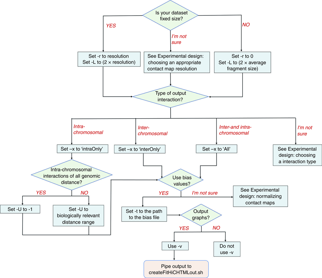
Flowchart of FitHiC2 parameter and configuration setting choices.

python3 $FITHICDIR/fithic.py

–I $DATADIR/contactCounts/Rao_GM12878-primary-chr5_5kb.gz

–f $DATADIR/fragmentMappability/Rao_GM12878-primary-chr5_5kb.gz

–t $DATADIR/biasValues/Rao_GM12878-primary-chr5_5kb.gz

–r 5000

–o $DATADIR/fithicOutput/Rao_GM12878-primary-chr5_5kb

–l Rao_GM12878-primary-chr5_5kb

–U 1000000

–L 15000

–v

? TROUBLESHOOTING

• 7To create an HTML report summarizing and depicting the output of FitHiC2, run the following commands. The output of the command below is an HTML report created in the output folder with the library name as its prefix.

  bash $FITHICDIR/utils/createFitHiCHTMLout.sh Rao_GM12878–primary–chr5_5kb 1 $DATADIR/fithicOutput/Rao_GM12878–primary–chr5_5kb

  DESCRIPTION:

  bash createFitHiCHTMLout.sh [Library Name] [No. of passes] [Fit-Hi-C output folder]

  [Library Name]The library name (-l option) used during Fit-Hi-C’s run

  [No. of passes]The number of spline passes conducted by the Fit-Hi-C run

  [Fit-Hi-C output folder]Path to the output folder for that Fit-Hi-C run (-o option)

  ? TROUBLESHOOTING

Running FitHiC2: yeast ● Timing ~10 min

• 8Then, conduct the analysis on the Duan yeast dataset, with the following command:

  python3 $FITHICDIR/fithic.py

  –i $DATADIR/contactCounts/Duan_yeast_EcoRI.gz

  –f $DATADIR/fragmentMappability/Duan_yeast_EcoRI.gz

  –t $DATADIR/biasValues/Duan_yeast_EcoRI.gz

  –r 0

  –o $DATADIR/fithicOutput/Duan_yeast_EcoRI

  –l Duan_yeast_EcoRI

  –p 2

  –v

  ? TROUBLESHOOTING

• 9To generate an HTML report for this run, use the commands below. Users will note that the HTML outputs differ in more than content. For this sample, we have two new graphs included in the top of the report. These graphs are only outputted when multiple spline passes are run and showcase the difference between the first and last spline pass. An example of the first few lines of this file is shown in Box 5.

  bash $FITHICDIR/utils/createFitHiCHTMLout.sh Duan_yeast_EcoRI 2 $DATADIR/fithicOutput/Duan_yeast_EcoRI

  ? TROUBLESHOOTING

Running FitHiC2: 40-kb whole-genome human, intra-chromosomal contacts ● Timing ~1 h 30 min

• 10Now, analyze the 40-kb IMR90 whole-genome dataset using different flags to simulate multiple use cases. The first is studying intra-chromosomal contacts only.

  python3 $FITHICDIR/fithic.py

  –i $DATADIR/contactCounts/Dixon_IMR90-wholegen_40kb.gz

  –f $DATADIR/fragmentMappability/Dixon_IMR90-wholegen_40kb.gz

  –t $DATADIR/biasValues/Dixon_IMR90-wholegen_40kb.gz

  –r 40000

  –o $DATADIR/fithicOutput/Dixon_IMR90-wholegen_40kb/intraChromosomal

  –l Dixon_IMR90-wholegen_40kb-intraChromosomal

  –U 10000000

  –L 80000

  –x intraOnly

  –v

  ? TROUBLESHOOTING

Running FitHiC2: 40-kb whole-genome human, inter-chromosomal contacts ● Timing ~ 4 h

• 11Now, analyze inter-chromosomal contacts.

  python3 $FITHICDIR/fithic.py

  –I $DATADIR/contactCounts/Dixon_IMR90-wholegen_40kb.gz

  –f $DATADIR/fragmentMappability/Dixon_IMR90-wholegen_40kb.gz

  –t $DATADIR/biasValues/Dixon_IMR90-wholegen_40kb.gz

  –r 40000

  –o $DATADIR/fithicOutput/Dixon_IMR90-wholegen_40kb/interChromosomal

  –l Dixon_IMR90-wholegen_40kb-interChromosomal

  –U 10000000

  –L 80000

  –x interOnly

  –v

Running FitHiC2: 40-kb whole-genome human, all contacts ● Timing ~ 4 h

• 12Finally, run the analysis below to identify all interactions, inter-chromosomal and intra-chromosomal.

  python3 $FITHICDIR/fithic.py

  –I $DATADIR/contactCounts/Dixon_IMR90-wholegen_40kb.gz

  –f $DATADIR/fragmentMappability/Dixon_IMR90-wholegen_40kb.gz

  –t $DATADIR/biasValues/Dixon_IMR90-wholegen_40kb.gz

  –r 40000

  –o $DATADIR/fithicOutput/Dixon_IMR90-wholegen_40kb/All

  –l Dixon_IMR90-wholegen_40kb-All

  –U 10000000

  –L 80000

  –x All

  –v

  ? TROUBLESHOOTING

  ■ PAUSE POINT The next series of steps involves post-processing and analyzing FitHiC2’s output. We encourage users to save copies of the previous results elsewhere so they may freely manipulate the output without fear of erasing FitHiC2’s results.

Merging significant interactions ● Timing ~40 min

• 13To merge spatially close, significant interactions from FitHiC2, we make use of another utility that FitHiC2 provides. Specifically, we call the script merge-filter.sh.

  bash merge-filter.sh $DATADIR/fithicOutput/Rao_GM12878-primary-chr5_5kb/Rao_GM12878-primary-chr5_5kb.spline_pass1.res5000.significances.txt.gz 5000 $DATADIR/fithicOutput/Rao_GM12878-primary-chr5_5kb/Rao_GM12878-primary-chr5_5kb-merged.gz0.01

  DESCRIPTION:

  bash merge-filter.sh [inputFile] [resolution] [outputDirectory] [fdr]

  [inputFile]Input file of Fit-Hi-C interactions

  [resolution]Resolution used for run

  [outputFile]Path to output file to dump contacts

  [fdr]FDR to use when subsetting interactions

  ? TROUBLESHOOTING

Analyzing FitHiC2 output ● Timing ~10 min

▲ CRITICAL We can now visualize the FitHiC2 interaction calls through the WashU Epigenome Browser. Below we show an example using the GM12878 5-kb FitHiC2 calls, using an FDR (Q value) threshold of 1 × 10⁻¹⁰. A similar procedure is to be employed for any FitHiC2 output, to output a new file formatted specifically for the WashU Epigenome Browser.

• 14Run this one-line awk command, and note the value of ‘q’:

  Zcat $DATADIR/fithicOutput/Rao_GM12878-primary-chr5_5kb/Rao_GM12878–primary–chr5_5kb.spline_pass1.res5000.significances.txt.gz | awk –v q=1e–10 ‘{if($7 <q) {print $0}}’ | awk –F[‘\t’] ‘{if(NR>1) {if($NF>0) {print $1”\t”($2−1)”\t”($2+1)”\t”$3”:”($4−1)”-“($4+1)”,”(−log($7)/log(10))”\t”(NR−1)”\t.”}else { print $1”\t” ($2−1)”\t”($2+1)”\t”$3”:”($4−1)”-“($4+1)”,500\t”(NR−1)”\t.”}}}’ | sort –k1,1 –k2,2n > $DATADIR/fithicOutput/Rao_GM12878-primary-chr5_5kb/washu_browser_format.bed

• 15Using bgzip and tabix (tools included in htslib; installation instructions found here: www.htslib.org/download/), run the following commands on the outputted bed file:

  Bgzip $DATADIR/fithicOutput/Rao_GM12878-primary-chr5_5kb/washu_browser_format.bed

  tabix –f –p bed $DATADIR/fithicOutput/Rao_GM12878-primary-chr5_5kb/washu_browser_format.bed.gz

• 16Go to epigenomegateway.wustl.edu/browser and select the correct organism and genome; in our case, Human and hg19.
• 17Click ‘Tracks’ and then ‘Upload Local Track’.
• 18Select ‘longrange’ when selecting the option for ‘Choose track file type’ and locate the created output files (found at $DATADIR/fithicOutput/Rao_GM12878-primary-chr5_5kb/washu_browser_format.bed.gz and /washu_browser_format.bed.gz.tbi). Note that both of these files need to be selected and uploaded together.
• 19Click the red ‘X’ in the top right and then left-click the name of the added track. Click ‘Display mode:’ and change the option to ‘ARC’.
• 20Your results should now be displayed as a track in the browser. Try clicking the coordinate location and typing in the following region: chr5:171842908–174092908. An example of what should be depicted is shown in Box 6. More detailed information about how to navigate the Epigenome Browser can be found at: https://epigenomegateway.readthedocs.io/en/latest.

Troubleshooting

Troubleshooting advice can be found in Table 2.

Table 2 |.

Troubleshooting table

Step	Problem	Possible reason	Solution
Materials	Incorrect version of Fit-Hi-C being installed (not 2.0.x)	Old version of Python is being used.	Ensure that you are using Python3.6’s pip command.
1–13	‘No such file or directory’	Not in correct working directory	Make sure that the path to the script being run is correct.
1, 3, 7	‘Invalid argument’	Arguments in incorrect order	Follow exact order of arguments as outlined in Procedure.
3	‘python2 not found’	Internal script requires Python2.	Install Python2 from the official Python distributors or Anaconda.
4	‘Nan’ values present in bias file	KR algorithm failed to converge.	Increase value of -x.
6	Code takes too long.	Running HiCKRy on the IMR 5-kb dataset is too slow on a personal laptop.	Utilize a high-performance compute cluster, or skip this step.
7	HTML contains no graphs.	Ensure that FitHiC2 was run with -v option.	Rerun FitHiC2 with -v option.
8	‘A theoretically impossible result was found during the iteration process for finding a smoothing spline with fp = s: s too small.’	Too many spline passes have been computed; spline is now undefined.	Decrease number of spline passes.
8–11	‘Argument required’	Not all required arguments have been passed to FitHiC2.	Ensure that all of the following arguments are explicitly defined: —interactions, —fragments, —outdir, —resolution.

Timing

The total time of the Procedure for all of the given use cases is ~12 h including preprocessing. This number decreases to ~4 h if different use cases are run in parallel. The steps that require the most time are Steps 8–11 (dealing with running FitHiC2). The runtime for these steps is dependent on the resolution of Hi-C data and the options chosen by the user as described in the article.

Anticipated results

The protocol results in bin statistics, graphs and statistical confidence estimates appended to the end of the contact maps file provided. Additional post-processing may be conducted to generate an HTML report (Box 6) summarizing this information and to visualize the results on the WashU Epigenome Browser (Box 7).

The resulting confidence estimates or statistically significant interactions may be intersected with an external browser extensible data (BED) file to gather a subset of interactions such as those from gene promoters or peaks from ChIP-seq analysis. In addition, the set of significant interactions can be summarized to find interaction hubs, which are defined as top-k regions with the highest number of stringent interactions.

Reporting Summary

Further information on research design is available in the Nature Research Reporting Summary linked to this article.

Data availability

FitHiC2 calls for different Hi-C datasets as well as processed files from published data that are used as references are provided in the Zenodo repository: https://doi.org/10.5281/zenodo.3380589³⁵.

Code availability

The source code and the documentation of FitHiC2 are publicly available through GitHub: https://github.com/ay-lab/fithic. An executable version is also provided on Code Ocean at https://codeocean.com/capsule/4528858/³⁶. The source code is distributed under the MIT license at https://opensource.org/licenses/MIT.

References

- 1.Bickmore WA The spatial organization of the human genome. Annu. Rev. Genomics Hum. Genet. 14, 67–84 (2013). [DOI] [PubMed] [Google Scholar]
- 2.Dekker J, Marti-Renom MA & Mirny LA Exploring the three-dimensional organization of genomes: interpreting chromatin interaction data. Nat. Rev. Genet. 14, 390–403 (2013). [DOI] [PMC free article] [PubMed] [Google Scholar]
- 3.Quinodoz SA et al. Higher-order inter-chromosomal hubs shape 3D genome organization in the nucleus. Cell 174, 744–757.e24 (2018). [DOI] [PMC free article] [PubMed] [Google Scholar]
- 4.Rao SS et al. A 3D map of the human genome at kilobase resolution reveals principles of chromatinlooping. Cell 159, 1665–1680 (2014). [DOI] [PMC free article] [PubMed] [Google Scholar]
- 5.Duan Z et al. A three-dimensional model of the yeast genome. Nature 465, 363–367 (2010). [DOI] [PMC free article] [PubMed] [Google Scholar]
- 6.Kalhor R, Tjong H, Jayathilaka N, Alber F & Chen L. Genome architectures revealed by tethered chromosome conformation capture and population-based modeling. Nat. Biotechnol. 30, 90–98 (2011). [DOI] [PMC free article] [PubMed] [Google Scholar]
- 7.Lieberman-Aiden E et al. Comprehensive mapping of long-range interactions reveals folding principles ofthe human genome. Science 326, 289–293 (2009). [DOI] [PMC free article] [PubMed] [Google Scholar]
- 8.Stadhouders R et al. Transcription regulation by distal enhancers: who’s in the loop? Transcription 3, 181–186 (2012). [DOI] [PMC free article] [PubMed] [Google Scholar]
- 9.Ay F & Noble WS Analysis methods for studying the 3D architecture of the genome. Genome Biol. 16, 183 (2015). [DOI] [PMC free article] [PubMed] [Google Scholar]
- 10.Lajoie BR, Dekker J & Kaplan N. The hitchhiker’s guide to Hi-C analysis: practical guidelines. Methods 72, 65–75 (2015). [DOI] [PMC free article] [PubMed] [Google Scholar]
- 11.Servant N et al. HiC-Pro: an optimized and flexible pipeline for Hi-C data processing. Genome Biol. 16, 259 (2015). [DOI] [PMC free article] [PubMed] [Google Scholar]
- 12.Imakaev M et al. Iterative correction of Hi-C data reveals hallmarks of chromosome organization. Nat. Methods 9, 999–1003 (2012). [DOI] [PMC free article] [PubMed] [Google Scholar]
- 13.Yaffe E & Tanay A. Probabilistic modeling of Hi-C contact maps eliminates systematic biases tocharacterize global chromosomal architecture. Nat. Genet. 43, 1059–1065 (2011). [DOI] [PubMed] [Google Scholar]
- 14.Ay F, Bailey TL & Noble WS Statistical confidence estimation for Hi-C data reveals regulatory chromatin contacts. Genome Res. 24, 999–1011 (2014). [DOI] [PMC free article] [PubMed] [Google Scholar]
- 15.Bhattacharyya S, Chandra V, Vijayanand P & Ay F. Identification of significant chromatin contacts from HiChIP data by FitHiChIP. Nat. Commun. 10, 4221 (2019). [DOI] [PMC free article] [PubMed] [Google Scholar]
- 16.Knight PA & Ruiz D. A fast algorithm for matrix balancing. IMA J. Numer. Anal. 33, 1029–1047 (2013). [Google Scholar]
- 17.Benjamini Y & Hochberg Y. Controlling the false discovery rate: a practical and powerful approach tomultiple testing. J. R. Stat. Soc. Series B Stat. Methodol. 57, 289–300 (1995). [Google Scholar]
- 18.Ay F et al. Three-dimensional modeling of the P. falciparum genome during the erythrocytic cycle reveals a strong connection between genome architecture and gene expression. Genome Res. 24, 974–988 (2014). [DOI] [PMC free article] [PubMed] [Google Scholar]
- 19.Wang C et al. Genome-wide analysis of local chromatin packing in Arabidopsis thaliana. Genome Res. 25, 246–256 (2015). [DOI] [PMC free article] [PubMed] [Google Scholar]
- 20.Wang M et al. Asymmetric subgenome selection and cis-regulatory divergence during cotton domestication. Nat. Genet. 49, 579–587 (2017). [DOI] [PubMed] [Google Scholar]
- 21.Ay F et al. Identifying multi-locus chromatin contacts in human cells using tethered multiple 3C. BMC Genomics 16, 121 (2015). [DOI] [PMC free article] [PubMed] [Google Scholar]
- 22.Bunnik EM et al. Comparative 3D genome organization in apicomplexan parasites. Proc. Natl Acad. Sci. USA 116, 3183–3192 (2019). [DOI] [PMC free article] [PubMed] [Google Scholar]
- 23.Forcato M et al. Comparison of computational methods for Hi-C data analysis. Nat. Methods 14, 679–685 (2017). [DOI] [PMC free article] [PubMed] [Google Scholar]
- 24.Hwang YC et al. HIPPIE: a high-throughput identification pipeline for promoter interacting enhancer elements. Bioinformatics 31, 1290–1292 (2015). [DOI] [PMC free article] [PubMed] [Google Scholar]
- 25.Lun AT & Smyth GK diffHic: a Bioconductor package to detect differential genomic interactions in Hi-C data. BMC Bioinformatics 16, 258 (2015). [DOI] [PMC free article] [PubMed] [Google Scholar]
- 26.Mifsud B et al. GOTHiC, a probabilistic model to resolve complex biases and to identify real interactions inHi-C data. PLoS One 12, e0174744 (2017). [DOI] [PMC free article] [PubMed] [Google Scholar]
- 27.Carty M et al. An integrated model for detecting significant chromatin interactions from high-resolution Hi-C data. Nat. Commun. 8, 15454 (2017). [DOI] [PMC free article] [PubMed] [Google Scholar]
- 28.Dixon JR et al. Topological domains in mammalian genomes identified by analysis of chromatin interactions. Nature 485, 376–380 (2012). [DOI] [PMC free article] [PubMed] [Google Scholar]
- 29.Fulco CP et al. Activity-by-contact model of enhancer–promoter regulation from thousands of CRISPR perturbations. Nat. Genet. 51, 1664–1669 (2019). [DOI] [PMC free article] [PubMed] [Google Scholar]
- 30.Chakraborty A & Ay F. Identification of copy number variations and translocations in cancer cells from Hi-C data. Bioinformatics, 10.1093/bioinformatics/btx664 (2017). [DOI] [PMC free article] [PubMed] [Google Scholar]
- 31.Dixon JR et al. Integrative detection and analysis of structural variation in cancer genomes. Nat. Genet. 50, 1388–1398 (2018). [DOI] [PMC free article] [PubMed] [Google Scholar]
- 32.Jin F et al. A high-resolution map of the three-dimensional chromatin interactome in human cells. Nature 503, 290–294 (2013). [DOI] [PMC free article] [PubMed] [Google Scholar]
- 33.Yardimci GG et al. Measuring the reproducibility and quality of Hi-C data. Genome Biol. 20, 57 (2019). [DOI] [PMC free article] [PubMed] [Google Scholar]
- 34.Huang J, Marco E, Pinello L & Yuan GC Predicting chromatin organization using histone marks. Genome Biol. 16, 162 (2015). [DOI] [PMC free article] [PubMed] [Google Scholar]
- 35.Kaul A, Bhattacharyya S & Ay F. Identifying statistically significant chromatin contacts from Hi-C data with FitHiC2. Zenodo, 10.5281/zenodo.3380589 (2019). [DOI] [PMC free article] [PubMed] [Google Scholar]
- 36.Kaul A, Bhattacharyya S & Ay F. Identifying statistically significant chromatin contacts from Hi-C data with FitHiC2. Code Ocean, 10.24433/CO.5589539.v2 (2019). [DOI] [PMC free article] [PubMed] [Google Scholar]
- 37.Durand NC et al. Juicer provides a one-click system for analyzing loop-resolution Hi-C experiments. Cell Syst. 3, 95–98 (2016). [DOI] [PMC free article] [PubMed] [Google Scholar]
- 38.Yardimci GG & Noble WS Software tools for visualizing Hi-C data. Genome Biol. 18, 26 (2017). [DOI] [PMC free article] [PubMed] [Google Scholar]
Associated Data
This section collects any data citations, data availability statements, or supplementary materials included in this article.
Supplementary Materials
Data Availability Statement