Prediction Accuracy Measures for a Nonlinear Model and for Right-Censored Time-to-Event Data

Abstract

This article develops a pair of new prediction summary measures for a nonlinear prediction function with right-censored time-to-event data. The first measure, defined as the proportion of explained variance by a linearly corrected prediction function, quantifies the potential predictive power of the nonlinear prediction function. The second measure, defined as the proportion of explained prediction error by its corrected prediction function, gauges the closeness of the prediction function to its corrected version and serves as a supplementary measure to indicate (by a value less than 1) whether the correction is needed to fulfill its potential predictive power and quantify how much prediction error reduction can be realized with the correction. The two measures together provide a complete summary of the predictive accuracy of the nonlinear prediction function. We motivate these measures by first establishing a variance decomposition and a prediction error decomposition at the population level and then deriving uncensored and censored sample versions of these decompositions. We note that for the least square prediction function under the linear model with no censoring, the first measure reduces to the classical coefficient of determination and the second measure degenerates to 1. We show that the sample measures are consistent estimators of their population counterparts and conduct extensive simulations to investigate their finite sample properties. A real data illustration is provided using the PBC data. Supplementary materials for this article are available online. An R package PAmeasures has been developed and made available via the CRAN R library. Supplementary materials for this article are available online.

1. Introduction

In this article, we study prediction accuracy measures for a nonlinear prediction function based on a possibly misspecified nonlinear model with right-censored time-to-event data. By far, the most commonly used prediction accuracy measure for a linear model is the R² statistic, or coefficient of determination. Let Y be a real-valued random variable and X be a vector of p real-valued explanatory random variables or covariates. Assume that one observes a random sample (Y₁, X₁),...,(Y_n, X_n) from the distribution of (Y, X). The R² statistic is defined as

$$R^2=1-\frac{{\sum }_{i=1}^n{\left(Y_i-{\widehat{Y}}_i\right)}^2}{{{\sum }_{i=1}^n\left(Y_i-\overline{Y}\right)}^2},$$ (1)

where ${\widehat{Y}}_i=a+b^T{X}_i$ is the least squares predicted value for subject i. The R² statistic has the straightforward interpretation as the proportion of variation of Y, which is explained by the least squares prediction function due to the following variance decomposition:

$$\sum _{i=1}^n{\left(Y_i-\overline{Y}\right)}^2=\sum _{i=1}^n{\left({\widehat{Y}}_i-\overline{Y}\right)}^2+\sum _{i=1}^n{\left(Y_i-{\widehat{Y}}_i\right)}^2.$$ (2)

$$\text{total variation}=\text{explained variation}+\text{unexplained variation}$$

Despite its popularity in linear regression, the above R² statistic is not readily applicable to a nonlinear model since the decomposition (2) no longer holds. In the past decades, much efforts have been devoted to extending the R² statistic to nonlinear models. Among others, the pseudo, R² statistics for a nonlinear model include likelihood-based measures (Goodman 1971; McFadden et al. 1973; Maddala 1986; CoxandSnell 1989; Magee 1990; Nagelkerke 1991), information-based measures (McFadden et al. 1973; Kent 1983), ranking-based measures (Harrell et al. 1982), variation-based measures (Theil 1970; Efron 1978; Haberman 1982; Hilden 1991; Cox and Wermuth 1992; Ash and Shwartz 1999), and the multiple correlation coefficient measure (Mittlböck and Schemper 1996; Zheng and Agresti 2000). However, none of the existing pseudo R² measures are motivated directly from a variance decomposition and none have received the same widespread acceptance as the classical R² for linear regression. Interested readers are referred to Zheng and Agresti (2000) for an excellent survey of existing pseudo R² measures and further references.

In this article, we first develop a pair of new prediction accuracy measures for a nonlinear prediction function of an individual response. We begin with defining population prediction accuracy measures. Based on a variance decomposition, we define a ρ² measure as the proportion of the explained variance of Y by a corrected prediction function, which is shown to coincide with the squared multiple correlation coefficient between the response and the predicted response. Because it describes the proportion of the explained variance by its corrected prediction function, ρ² measures the potential predictive power of the predictive function and thus by itself is not sufficient to summarize the prediction accuracy of the prediction function. As a remedy, we introduce another parameter, λ², defined as the proportion of prediction error explained by the corrected prediction function based on a prediction error decomposition, to measure how close the prediction function is to its corrected version and quantifies how much prediction error reduction is realized with the correction. The two parameters capture complementary information regarding the predictive accuracy of the prediction function and provide a complete summary of its predictive power. We further develop sample versions of the variance and prediction error decompositions based on uncensored data, define the corresponding sample prediction accuracy measures, namely R² and L², and establish their asymptotic properties. It is worth noting that for the least squares prediction function under the linear model, L² always degenerates to 1 and thus only R² is needed to describe its predictive accuracy.

We further extend the proposed prediction accuracy measures to event time models with right-censored time-to-event data. Note that even for the linear model, it is not clear how to extend the R² statistic defined in (1) to right-censored data since some of the Y values are not observed. A variety of pseudo R² measures and other loss functions have been proposed for event time models with right-censored data (Kent and O’Quigley 1988; Korn and Simon 1990; Graf et al. 1999; Schemper and Henderson 2000; Royston and Sauerbrei 2004; O’Quigley, Xu, and Stare 2005; Stare, Perme, and Henderson 2011). For example, the EV option in the SAS PHREG procedure gives a generalized R² measure proposed by Schemper and Henderson (2000) for Cox’s (1972) proportional hazards model. Amore recent proposal by Stare, Perme, and Henderson (2011) uses explained rank information, which is applicable to a wide range of event time models. Stare, Perme, and Henderson (2011) also gave a thorough literature review of prediction accuracy measures for event time models. We highlight that for linear regression, none of the existing pseudo R² measures for right-censored data reduce to the classical R² statistic in the absence of censoring. Moreover, under a correctly specified model, they do not converge to the nonparametric population R² value ${\rho }_{NP}^2\equiv \text{var}(E(Y|X))/\text{var}(Y)$, the proportion of the explained variance by $E\left(Y\right|X)$, as the sample size grows large. Finally, as illustrated in Section 4 (Table 1), the pseudo R² measures of Schemper and Henderson (2000) and Stare, Perme, and Henderson(2011) may fail to distinguish between Cox’s models with the same regression coefficients but different baseline hazards: they could remain constant for different Cox’s models as ${\rho }_{NP}^2$ varies from 0 to 1. In Section 3, we propose right-censored sample versions of R² and L² by deriving a variance decomposition and a prediction error decomposition for right-censored data and show that they are consistent estimators of the population parameters ρ² and λ². The proposed measures possess multiple appealing properties that most existing pseudo R² measures do not have. First, for the linear model with no censoring, our R² statistic reduces to the classical coefficient of determination and L² degenerates to 1. Second, when the prediction function is the conditional mean response based on a correctly specified model, our R² statistic is a consistent estimate of the nonparametric coefficient of determination ${\rho }_{NP}^2$, and L² converges to 1 as the sample size grows to infinity. Third, our method is applicable to a variety of event time models including the Cox proportional hazards model, accelerated failure time models, additive risk models, threshold regression model, proportional odds model, and transformation models, with time-independent covariates and independently right-censored data. Fourth, our measures are defined without requiring the prediction model to be correctly specified. Finally, the proposed R² statistic provides a natural benchmark to compare the potential prediction power between prediction models that are not necessarily nested or correctly specified as illustrated in the real data example in Section 5.

Table 1.

Simulated population proportion $\left({\rho }_{\text{NP}}^2\right)$ of explained variance by the Cox (1972) model and population ($R_{\text{SPH}}^2$ and $R_{\text{SH}}^2$ of Schemper and Henderson (2000) and Stare, Perme, and Henderson (2011).

Model	β	υ	${\rho }_{\text{NP}}^2$	$R_{\text{SPH}}^2$	$R_{\text{SH}}^2$
1	0.1	0.5	0.07	0.23	0.10
2	0.1	1	0.14	0.23	0.10
3	0.1	10	0.15	0.23	0.10
4	0.2	0.5	0.09	0.38	0.28
5	0.2	1	0.27	0.38	0.28
6	0.2	10	0.40	0.38	0.28
7	0.5	0.5	0.09	0.49	0.49
8	0.5	1	0.33	0.49	0.49
9	0.5	10	0.80	0.49	0.49

The rest of the article is organized as follows. In Section 2.1, we define a pair of population prediction accuracy measures for a nonlinear prediction function by deriving a variance decomposition and a prediction error decomposition. Sample measures based on independent and identically distributed complete data are then proposed and studied in Section 2.2. Section 3 extends these measures to event time models with right-censored data. Section 4 presents simulations to illustrate potential weaknesses of some existing pseudo R² proposals for right-censored data and investigate the finite sample performance of the proposed measures. A real data example is given in Section 5. Further remarks are provided in Section 6. Additional lemmas, all theoretical proofs, and more numerical results are collected in the supplementary materials.

2. Prediction Accuracy Measures for a Nonlinear Model

Denote by $F(y|x)=P(Y\le y|X=x)$ the true conditional distribution function of Y given X = x. Consider a regression model of Y on X described by a family of conditional distribution functions $\mathcal{M}=\left\{F_{\theta }(y|x):\theta \in \mathrm{\Theta }\right\}$, where θ is either finite or infinite dimensional. For example, $F_{\theta }(y|x)=\mathrm{\Phi }(y-\alpha -{\beta }^{T}x)/\sigma )$ for the linear regression model with a normal N(0, σ²) error, where θ = (α, β^T, σ²) and Φ is the standard normal cumulative distribution function. For the Cox (1972) proportional hazards model, $F_{\theta }(y|x)=1-{\left\{1-F_0(y)\right\}}^{\exp \left({\beta }^{T}x\right)}$ where θ = (β, F₀) consists of a finite dimensional regression parameter β and an infinite dimensional unknown baseline distribution function F₀. Model $\mathcal{M}$ is said to be misspecified if it does not include the true conditional distribution function F(y|x) as a member.

For any $\theta \in \mathrm{\Theta }$, let $m_{\theta }(X)$ be a prediction function of Y obtained as a functional of $F_{\theta }(\cdot |X)$. Common examples of $m_{\theta }(X)$ include the conditional mean response $m_{\theta }(x)=\int yd{F}_{\theta }(y|x)$ and the conditional median response $m_{\theta }(x)=F_{\theta }^{-1}(0.5|x)$. Assume that $\widehat{\theta }$ is a sample statistic that converges to a limit ${\theta }^{*}$ as n grows to ∞. As discussed in the supplementary materials (Appendix A.1) ${\theta }^{*}$ is typically the true parameter value under a correctly specified model, and the parameter value that minimizes the Kullback-Leibler information criterion under a misspecified model.

Below, we first develop population prediction accuracy measures for $m_{{\theta }^{*}}(X)$, which can be regarded as the asymptotic accuracy measures for the predictive power of $m_{\widehat{\theta }}(x)$. Their sample versions for $m_{\widehat{\theta }}(X)$ will then be derived in a similar fashion.

2.1. Population Prediction Accuracy Measures

For any p-variate function P(x), define MSPE(P(X)) = E{Y − P(X)}². as the mean squared prediction error of P(X) for predicting Y. In general, it would be desirable for a prediction function P(X) of Y to possess at least the following properties: (i) $E\{P(X)\}={\mu }_Y$ and (ii) MSPE $(P(X))\le \text{MSPE}\left({\mu }_Y\right)$, where ${\mu }_Y=E(Y)$ is the best prediction among all constant (non-informative) predictions of Y as measured by MSPE. However, such minimal requirements are not always met by $m_{{\theta }^{*}}(X)$ when the model $\mathcal{M}$ is possibly misspecified or when the prediction is not based on the conditional mean response. Below, we introduce a linearly corrected prediction function, which always meets the above requirements (i) and (ii) and is pivotal to assessing the predictive accuracy of $m_{{\theta }^{*}}(X)$.

Definition 2.1.

The linearly corrected prediction function of $m_{{\theta }^{*}}(X)$ is defined as

$$\begin{gathered} m_{{\theta }^{*}}^{(c)}(X)=\tilde{a}+\tilde{b}{m}_{{\theta }^{*}}(X)={\mu }_Y \\ +\frac{\text{cov}\left(Y,m_{{\theta }^{*}}(X)\right)}{\text{var}\left(m_{{\theta }^{*}}(X)\right)}\left[m_{{\theta }^{*}}(X)-E\left\{m_{{\theta }^{*}}(X)\right\}\right], \end{gathered}$$ (3)

where $(\tilde{a},\tilde{b})=\arg {\min }_{\alpha ,\beta }E{\left\{Y-\left(\alpha +\beta m_{{\theta }^{*}}(X)\right)\right\}}^2$.

It is easy to see that $m_{{\theta }^{*}}^{(c)}(X)$ satisfies the above mentioned requirements (i) and (ii) and that $MPSE\left(m_{{\theta }^{*}}^{(c)}(X)\right)\le MPSE\left(m_{{\theta }^{*}}(X)\right)$. More importantly, by Lemma A.1 (supplementary materials), $m_{{\theta }^{*}}^{(c)}(X)$ facilitates the following variance and prediction error decompositions:

$$\text{var}(Y)=E{\left\{m_{{\theta }^{*}}^{(c)}(X)-{\mu }_Y\right\}}^2+E{\left\{Y-m_{{\theta }^{*}}^{(c)}(X)\right\}}^2,$$ (4)

and

$$\begin{gathered} \text{MSPE}\left(m_{{\theta }^{*}}(X)\right)=E{\left\{Y-m_{{\theta }^{*}}^{(c)}(X)\right\}}^2 \\ +E{\left\{m_{{\theta }^{*}}^{(c)}(X)-m_{{\theta }^{*}}(X)\right\}}^2, \end{gathered}$$ (5)

which lead to the following prediction accuracy measures for $m_{{\theta }^{*}}(X)$.

Definition 2.2.

Define

$${\rho }_{m_{{\theta }^{*}}}^2=1-\frac{E{\left\{Y-m_{{\theta }^{*}}^{(c)}(X)\right\}}^2}{\text{var}(Y)}=\frac{E{\left\{m_{{\theta }^{*}}^{(c)}(X)-{\mu }_Y\right\}}^2}{\text{var}(Y)},$$ (6)

to be the proportion of the variance of Y, that is, explained by $m_{{\theta }^{*}}^{(c)}(X)$, and

$${\lambda }_{m_{\theta }*}^2=\frac{\text{MSPE}(m_{{\theta }^{*}}^{(c)}(X))}{\text{MSPE}\left(m_{{\theta }^{*}}(X)\right)}=1-\frac{E{\left\{m_{{\theta }^{*}}^{(c)}(X)-m_{{\theta }^{*}}(X)\right\}}^2}{\text{MSPE}\left(m_{{\theta }^{*}}(X)\right)}.$$ (7)

to be the proportion of the MSPE of $m_{{\theta }^{*}}(X)$, that is, explained by $m_{{\theta }^{*}}^{(c)}(X)$.

Remark 2.1 (Interpretation of ${\rho }_{m_{{\theta }^{*}}}^2$ and ${\lambda }_{m_{{\theta }^{*}}}^2$).

Define the L₂-distance between any two real-valued random variables ξ and η by $d_2(\xi ,\eta )={\left\{E{(\xi -\eta )}^2\right\}}^{\frac{1}{2}}$. Figure 1 depicts the geometric relationships between Y, μ_Y, $m_{{\theta }^{*}}(X)$, $m_{{\theta }^{*}}^{(c)}(X)$, and $E\left(Y\right|X)$, where $\mathcal{P}(X)$ denotes the space of all real-valued functions of X, $m_{{\theta }^{*}}^{(c)}(X)$ is the projection of Y onto the subspace of all linear functions of $m_{{\theta }^{*}}(X)$, and E(Y|X) is the projection of Y onto $\mathcal{P}(X)$.

Figure 1.

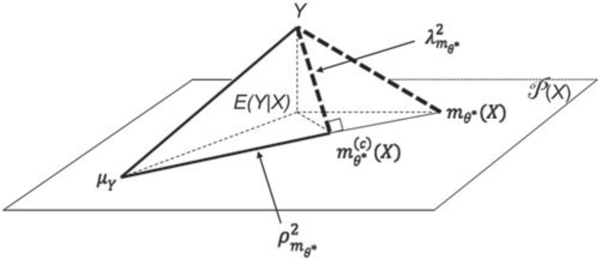
Geometric interpretation of ${\rho }_{m_{{\theta }^{*}}}^2$ and ${\lambda }_{m_{{\theta }^{*}}}^2$.

It is clear from Figure 1 that the variance decomposition (4) corresponds to the Pythagorean theorem for the triangle $\left(Y,m_{{\theta }^{*}}^{(c)}(X),{\mu }_Y\right)$, which leads to the definition of ${\rho }_{m_{\theta }*}^2$, and that the prediction error decomposition (5) is the Pythagorean theorem for $(Y,m_{{\theta }^{*}}^{(c)}(X),m_{{\theta }^{*}}(X))$, which defines ${\lambda }_{m_{{\theta }^{*}}}^2$. Therefore, ${\rho }_{m_{\theta }*}^2$ and ${\lambda }_{m_{{\theta }^{*}}}^2$ provide distinct, yet complementary information regarding the prediction accuracy of $m_{{\theta }^{*}}(X):{\rho }_{m_{{\theta }^{*}}}^2$ measures its potential predictive power through its corrected version $m_{{\theta }^{*}}^{(c)}(X)$, whereas ${\lambda }_{m_{{\theta }^{*}}}^2$ measures its closeness to $m_{{\theta }^{*}}^{(c)}(X)$ and quantifies how much prediction error reduction can be achieved with the correction. Together, they provide a complete summary of the predictive accuracy of $m_{{\theta }^{*}}(X)$. In practice, ${\rho }_{m_{\theta }*}^2$ should be used as the primary measure for the potential predictive power of $m_{{\theta }^{*}}(X)$, whereas ${\lambda }_{m_{\theta }*}^2$ should be used as a supplementary measure to indicate (by a value less than 1) if a linear correction is required for $m_{{\theta }^{*}}(X)$ to achieve its potential predictive power and how much prediction error reduction can be realized with the correction. Finally, L² is not to be confused as a lack-of-fit measure for model $\mathcal{F}$. Although $m_{{\theta }^{*}}(X)=E(Y|X)$ implies ${\lambda }_{m_{{\theta }^{*}}}^2=1$, ${\lambda }_{m_{{\theta }^{*}}}^2$ may also be 1 even if $m_{{\theta }^{*}}(X)\ne E(Y|X)$, as long as $m_{{\theta }^{*}}^{(c)}(X)=m_{{\theta }^{*}}(X)$. Hence, ${\lambda }_{m_{{\theta }^{*}}}^2=1$ simplyindicatesthat no linear correction is required for $m_{{\theta }^{*}}(X)$ to achieve it potential predictive power and does not necessarily imply that the model is correctly specified. This point is further illustrated by our simulation results in the supplementary materials (Appendix A.2.3, Figures A.4 and A.5: first row).

It is also seen from Figure 1 that the Pythagorean theorem for the triangle $\left(Y,E(Y|X),{\mu }_Y\right)$ corresponds to the following well-known variance decomposition

$$\text{var}(Y)=\text{var}(E(Y|X))+E(\text{var}(Y|X)).$$

We refer to

$${\rho }_{NP}^2\equiv 1-\frac{E{(Y-E(Y|X))}^2}{\text{var}(Y)}=\frac{\text{var}(\mu (X))}{\text{var}(Y)},$$ (8)

the proportion of explained variance by E(Y|X), as the non-parametric coefficient of determination. Note that $\sqrt{{\rho }_{NP}^2}$ is the “correlation ratio” studied previously by Renyi (1959).

The next theorem summarizes some fundamental properties of ${\rho }_{m_{{\theta }^{*}}}^2$ and ${\lambda }_{m_{{\theta }^{*}}}^2$

Theorem 2.1.

1. Let ρ(ξ, η) denote the correlation coefficient between two random variables ξ and η. Then, ${\rho }_{m_{{\theta }^{*}}}^2={\left[\rho \left(Y,m_{{\theta }^{*}}(X)\right)\right]}^2$;

2. (Linear prediction). Let BLUE(X) = a + b^TX be the best linear unbiased estimator (BLUE) of Y, where $(a,b)=\text{arg}{\min }_{\alpha ,\beta }{E\left\{Y-\left(\alpha +{\beta }^{T}X\right)\right\}}^2$. Then, (i) ${\text{BLUE}}^{(c)}(X)=\text{BLUE}(X)$, (ii) ${\lambda }_{\text{BLUE}}^2\equiv 1$, and (iii) ${\rho }_{\text{BLUE}}^2$ is equal to the population value of the classical coefficient of determination for linear regression;

3. If $m_{{\theta }^{*}}(X)=E(Y|X)$, then ${\lambda }_{m_{{\theta }^{*}}}^2\equiv 1$, and ${\rho }_{m_{{\theta }^{*}}}^2={\rho }_{NP}^2$, where ${\rho }_{NP}^2$ is defined in (8);

4. (Maximal ρ²) Let P(X) be the space of all p-variate functions Q(X) of X. Then ${\rho }_{NP}^2={\max }_{Q\in \mathcal{P}(X)}\left\{{\rho }_Q^2\right\}$.

2.2. Sample Prediction Accuracy Measures

Let (Y₁, X₁),...,(Y_n, X_n) be a random sample of (Y, X) and $\widehat{\theta }=\widehat{\theta }\left(Y_1,X_1,\dots ,Y_n,X_n\right)$ be a sample statistic. We next derive sample versions of ${\rho }_{m_{\theta }*}^2$ and ${\lambda }_{m_{\theta }*}^2$ for $m_{\widehat{\theta }}(X)$.

By Lemma A.2 (supplementary materials), we have the following sample version of the variance and prediction error decompositions:

$$\sum _{i=1}^n{\left(Y_i-\overline{Y}\right)}^2=\sum _{i=1}^n{\left(m_{\widehat{\theta }}^{(c)}\left(X_i\right)-\overline{Y}\right)}^2+\sum _{i=1}^n{\left(Y_i-m_{\widehat{\theta }}^{(c)}\left(X_i\right)\right)}^2,$$ (9)

and

$$\begin{gathered} \sum _{i=1}^n{\left(Y_i-m_{\widehat{\theta }}\left(X_i\right)\right)}^2 \\ =\sum _{i=1}^n{\left(Y_i-m_{\widehat{\theta }}^{(c)}\left(X_i\right)\right)}^2+\sum _{i=1}^n{\left(m_{\widehat{\theta }}^{(c)}\left(X_i\right)-m_{\widehat{\theta }}\left(X_i\right)\right)}^2, \end{gathered}$$ (10)

where $m_{\widehat{\theta }}^{(c)}(x)$ is the ordinary least squares regression function obtained by linearly regressing Y₁,..., Y_n on $m_{\widehat{\theta }}(X_1)$,...,$m_{\widehat{\theta }}(X_n)$.

The sample versions of ${\rho }_{m_{\theta }*}^2$ and ${\lambda }_{m_{\theta }*}^2$ are therefore, defined by

$$R_{m_{\widehat{\theta }}}^2=\frac{{{\sum }_{i=1}^n\left(m_{\widehat{\theta }}^{(c)}\left(X_i\right)-\overline{Y}\right)}^2}{{{\sum }_{i=1}^n\left(Y_i-\overline{Y}\right)}^2},$$ (11)

and

$$L_{m_{\widehat{\theta }}}^2=\frac{{\sum }_{i=1}^n{\left(Y_i-m_{\widehat{\theta }}^{(c)}\left(X_i\right)\right)}^2}{{{\sum }_{i=1}^n\left(Y_i-m_{\widehat{\theta }}\left(X_i\right)\right)}^2},$$ (12)

where $R_{m_{\widehat{\theta }}}^2$ is the proportion of variation of Y explained by $m_{\widehat{\theta }}^{(c)}(X)$ and $L_{m_{\widehat{\theta }}}^2$, is the proportion of prediction error of $m_{\widehat{\theta }}(X)$ explained by $m_{\widehat{\theta }}^{(c)}(X)$.

Remark 2.2.

Similar to Theorem 2.1(a), it can be shown that $R_{m_{\widehat{\theta }}}^2={\left\{r\left(Y,m_{\widehat{\theta }}(X)\right)\right\}}^2$, where $r\left(Y,m_{\widehat{\theta }}(X)\right)$ is the Pearson correlation coefficient between Y and $m_{\widehat{\theta }}(X)$. Furthermore, if $m_{\widehat{\theta }}(x)$ is the fitted least squares regression line from a linear model, then $L_{m_{\widehat{\theta }}}^2\equiv 1$ and $R_{m_{\widehat{\theta }}}^2$ is identical to the classical coefficient of determination for the linear model.

Below, we give the asymptotic properties of $R_{m_{\widehat{\theta }}}^2$, and $L_{m_{\widehat{\theta }}}^2$.

Theorem 2.2.

Assume conditions (C2)-(C4) of supplementary materials (Appendix A.1) hold. Then, as n → ∞

1. (Consistency) $R_{m_{\widehat{\theta }}}^2\stackrel{P}{\to }{\rho }_{m_{{\theta }^{*}}}^2$, and $L_{m_{\widehat{\theta }}}^2\stackrel{P}{\to }{\lambda }_{m_{{\theta }^{*}}}^2$;

2. (Asymptotic normality) $\sqrt{n}\left(R_{m_{\widehat{\theta }}}^2-{\rho }_{m_{{\theta }^{*}}}^2\right)\stackrel{d}{\to }N\left(0,{\sigma }_{\rho }^2\right)$, and $\sqrt{n}(L_{m_{\widehat{\theta }}}^2-{\lambda }_{m_{{\theta }^{*}}}^2)\stackrel{d}{\to }N\left(0,{\sigma }_{\lambda }^2\right)$, where ${\sigma }_{\rho }^2$ and ${\sigma }_{\lambda }^2$ are the asymptotic variances.

The asymptotic results allow one to assess the variability of the sample measures $R_{m_{\widehat{\theta }}}^2$ and $L_{m_{\widehat{\theta }}}^2$ and obtain confidence interval estimates for the corresponding population parameters. In practice, the bootstrap method (Efron and Tibshirani 1994) or a transformation-based method would be more appealing than the normal approximation method because the sampling distributions of $R_{m_{\widehat{\theta }}}^2$ and $L_{m_{\widehat{\theta }}}^2$ can be skewed, especially near 0 and 1.

3. Sample Prediction Accuracy Measures for Right-Censored Data

In this section, we extend the sample measures $R_{m_{\widehat{\theta }}}^2$ and $L_{m_{\widehat{\theta }}}^2$ defined by (11) and (12) to right-censored time-to-event data. Let T = min{Y, C} and δ = I(Y ≤ C), where C is an censoring random variable. Assume that one observes a right-censored sample of n independent and identically distributed triplets (T₁, δ₁, X₁),...,(T_n, δ_n, X_n) from the distribution of (T, δ, X).

Assume that $\widehat{\theta }=\widehat{\theta }\left(T_1,{\delta }_1,X_1,\dots ,T_n,{\delta }_n,X_n\right)$ is a sample statistic. The sample prediction accuracy measures defined in (11) and (12) are no longer directly applicable to right-censored data because Y is not observed on some subjects. In Lemma A.3 (supplementary materials), we show that

$$\begin{gathered} \sum _{i=1}^n{w}_i{\left\{T_i-{\overline{T}}^{(w)}\right\}}^2 \\ =\sum _{i=1}^n{w}_i{\left\{m_{\widehat{\theta }}^{(wc)}\left(X_i\right)-{\overline{T}}^{(w)}\right\}}^2+\sum _{i=1}^n{w}_i{\left\{T_i-m_{\widehat{\theta }}^{(wc)}\left(X_i\right)\right\}}^2, \end{gathered}$$ (13)

and

$$\begin{gathered} \sum _{i=1}^n{w}_i{\left\{T_i-m_{\widehat{\theta }}\left(X_i\right)\right\}}^2 \\ =\sum _{i=1}^n{w}_i{\left\{T_i-m_{\widehat{\theta }}^{(wc)}\left(X_i\right)\right\}}^2+\sum _{i=1}^n{w}_i{\left\{m_{\widehat{\theta }}^{(wc)}\left(X_i\right)-m_{\widehat{\theta }}\left(X_i\right)\right\}}^2, \end{gathered}$$ (14)

for any set of nonnegative weights w₁,…,w_n satisfying ${\sum }_{i=1}^n{w}_i=1$, where $m_{\widehat{\theta }}^{(wc)}(x)$ is the fitted regression function from the weighted least squares linear regression of Y₁,...,Y_n on $m_{\widehat{\theta }}\left(X_1\right),\dots ,m_{\widehat{\theta }}\left(X_n\right)$ with weight $W=\text{diag}\left\{w_1,\dots ,w_n\right\}$. Furthermore, in Lemma A.4 (supplementary materials), we will show that if

$$w_i=\frac{\frac{{\delta }_i}{\widehat{G}\left(T_i-\right)}}{{\sum }_{j=1}^n\frac{{\delta }_j}{\widehat{G}\left(T_j-\right)}},i=1,\dots ,n,$$ (15)

where $\widehat{G}$ is the Kaplan-Meier (Kaplan and Meier 1958)estimate of G(c) = P(C > c), then (13) and (14) can be regarded as the right-censored data analogs of the uncensored sample variance decomposition (9) and prediction error decomposition (10), respectively. These results lead to the following right-censored sample prediction accuracy measures.

Definition 3.1.

The right-censored sample versions of ${\rho }_{m_{{\theta }^{*}}}^2$ and ${\lambda }_{m_{{\theta }^{*}}}^2$ are defined by

$$R_{m_{\widehat{\theta }}}^2=\frac{{\sum }_{i=1}^n{w}_i{\left\{m_{\widehat{\theta }}^{(wc)}\left(X_i\right)-{\overline{T}}^{(w)}\right\}}^2}{{\sum }_{i=1}^n{w}_i{\left\{T_i-{\overline{T}}^{(w)}\right\}}^2},$$ (16)

and

$$L_{m_{\widehat{\theta }}}^2=\frac{{\sum }_{i=1}^n{w}_i{\left\{T_i-m_{\widehat{\theta }}^{(wc)}\left(X_i\right)\right\}}^2}{{\sum }_{i=1}^n{w}_i{\left\{T_i-m_{\widehat{\theta }}\left(X_i\right)\right\}}^2},$$ (17)

where the weight w_i’s are defined in (15).

The above defined $R_{m_{\widehat{\theta }}}^2$ can be interpreted as an approximate proportion of sample variance of Y explained by $m_{\widehat{\theta }}^{(wc)}(X)$ and $L_{m_{\widehat{\theta }}}^2$ an approximate proportion of sample mean squared prediction error of $m_{\widehat{\theta }}(X)$ explained by $m_{\widehat{\theta }}^{(wc)}(X)$. By definition, $0\le R_{m_{\widehat{\theta }}}^2\le 1$ and $0\le L_{m_{\widehat{\theta }}}^2\le 1$.

Theorem 3.1.

1. (Uncensored data). If there is no censoring, then formulas (16) and (17) reduce to the uncensored data definitions (11) and (12), respectively.

2. (Consistency). Assume conditions (C1)-(C5) hold. Then, as $n\to \infty ,R_{m_{\widehat{\theta }}}^2\stackrel{P}{\to }{\rho }_{m_{{\theta }^{*}}}^2,\text{and}{L}_{m_{\widehat{\theta }}}^2\stackrel{P}{\to }{\lambda }_{m_{{\theta }^{*}}}^2$.

3. (Asymptotic normality). Assume conditions (C1)-(C5) hold.Then, $\sqrt{n}\left(R_{m_{\widehat{\theta }}}^2-{\rho }_{m_{{\theta }^{*}}}^2\right)\stackrel{d}{\to }N\left(0,v_{\rho }^2\right)$ and $\sqrt{n}(L_{m_{\widehat{\theta }}}^2-{\lambda }_{m_{{\theta }^{*}}}^2)\stackrel{d}{\to }N\left(0,v_{\lambda }^2\right)$, as n → ∞, where $v_{\rho }^2$ and $v_{\lambda }^2$ are the asymptotic variances.

Remark 3.1.

Theorem 3.1 (b) and (c) are derived under condition (C1) of Appendix A.1 that C is independent of X and Y. In the next section, we demonstrate by simulation that the $R_{m_{\widehat{\theta }}}^2$ and $L_{m_{\widehat{\theta }}}^2$ measures are quite robust even if C depends the covariates X, unless the model is severely misspecified.

4. Simulations

We present several simulation studies to investigate the finite sample properties of the proposed prediction accuracy measures.

Simulation 1:

In this simulation, we use the population ${\rho }_{NP}^2$ defined by (8) as a benchmark to illustrate the properties and potential weaknesses of two existing R²-type measures $R_{SH}^2$ and $R_{SPH}^2$ for the Cox model proposed by Schemper and Henderson (2000) and Stare, Perme, and Henderson (2011), respectively. In the simulation, the event time Y is generated from a Cox proportional hazard model: $Y=H_0^{-1}\left[-\log (U)\times \exp \left(-{\beta }^{T}X\right)\right]$, where U ~ U(0,1), $H_0^{-1}(t)=2t^{\frac{1}{v}}$ is the inverse function of a Weibull cumulative hazard function $H_0(t)={(0.5t)}^v$, and X = 10 × Bernoulli(0.5). We consider nine data settings by varying β and v. We approximate the population ρ² value by averaging its sample R² values over 10 Monte Carlo samples of size n = 5000 with no censoring. The results are summarized by supplementary materials (Figure A.1 in Appendix A.2.1). Table 1 takes a snapshot of Figure A.1 for some selected settings.

Table 1 shows that for Cox’s models with the same baseline hazard (or v) but different hazard ratio (or β) (e.g., models 3, 6, 9), $R_{\text{SPH}}^2$ and $R_{\text{SH}}^2$ have produced the same rankings as ${\rho }_{\text{NP}}^2$ and thus have correctly reflected the relative predictive power between these models. However, both $R_{\text{SPH}}^2$ and $R_{\text{SH}}^2$ have failed to distinguish the predictive power between models with the same hazard ratio (or β) but different baseline hazard (or v). For example, they remain a constant 0.49 for models 7, 8, and 9 whose ${\rho }_{\text{NP}}^2$ values are 0.10, 0.33, and 0.80, respectively. This is not surprising for $R_{\text{SPH}}^2$ because it is a measure of the explained rank variation, that is, largely determined by β. However, the predictive power of the Cox model is determined by not only β, but also v, where the latter reflects the variability of the outcome variable and is not adequately accounted for by $R_{\text{SPH}}^2$. The $R_{\text{SH}}^2$ measure is observed to suffer from the same limitation although it is not as obvious to see from its definition.

Simulation 2:

This simulation investigates finite sample properties of the proposed R² and L² measures for the Cox model relative to their population values ρ² and λ² by varying the censoring rate (0%, 10%, 25%, 50%), sample size n (100,250,1000), and data generation setting (Weibull, Log-normal, Inverse Gaussian). For the Weibull setting, data are generated from a Weibull model $\log (Y)={\beta }^{T}X+\sigma W$, where β = 1, σ = 0.24, X ~ U(0,1), W ~ standard extreme value distribution. For the lognormal setting, data are generated from $\log (Y)={\beta }^{T}X+\sigma W$, where β = 1, σ = 0.27, X ~ U(0,1), W ~ N(0,1), and C ~ Weibull (shape = 1, shape = b) with b adjusted to produce a given censoring rate. For the inverse Gaussian setting, data are generated from Y ~ Inverse $\text{Gaussian (mean}=-\frac{e^{{\alpha }_0+{\alpha }_{1}X}}{{\beta }_0+{\beta }_{1}X},\text{shape}=e^{2*\left({\alpha }_0+{\alpha }_{1}X\right)})$, where α₀ = 3, α₁ = −2.5, β₀ = −1, β₁ = 0.6, X ~ U(0,1). For all three data settings, ρ² = 0.50, and censoring times are generated from C ~ Weibull (shape = 1, scale = b) with b adjusted to produce a given censoring rate.

We first examine the overall fit of the Cox model under each of the three data settings by displaying in Figure 2 the Cox-Snell residual plots for the Cox model based on the first 10 Monte Carlo replications (first row: Weibull; second row: log-normal AFT; third row: inverse Gaussian) with varying sample size (first column: n = 100; second column: n = 250; third column: n = 1000) and censoring rate, CR = 0%. The plots reveal no misspecification of the Cox model under the Weibull setting (first row), mild model misspecification under the log-normal setting (second row), serious model misspecification under the inverse Gaussian setting (third row).

Figure 2.

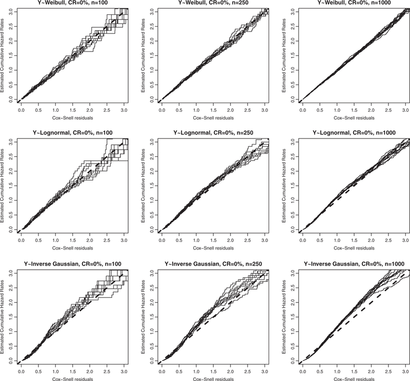
(Cox’s model with independent censoring; censoring rate, CR = 0%) Cox-Snell residual plot for the Cox model based on the first 10 Monte Carlo samples with censoring rate CR = 0%, varying sample size (first column: n = 100; second column: n = 250; third column: n = 1000), and varying data generation setting (first row: Weibull; second row: log-normal; third row: inverse Gaussian).

Figure 3 summarizes simulated R² (shaded box) and L² (unshaded box) values for the Cox model over 1000 Monte Carlo replications using boxplots by censoring rate (0%, 10%, 25%, 50%), sample size (100, 200, 1000), and data generation setting (upper panel: Weibull; middle panel: log-normal AFT; bottom panel: inverse Gaussian). The population values ρ² and λ² in Figure 3 are approximated by the averaged sample values over 100 Monte Carlo replications of sample size n = 5000 with no censoring. We observe from Figure 3 that for all three data settings, the proposed R² and L² estimate their population values well: their medians agree well with the population values and as expected, their variability increases as the censoring rate increases and decreases as the sample size increases.

Figure 3.

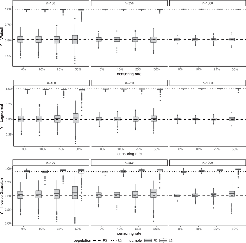
(Independent censoring) Boxplots of simulated R² (shaded box) and L² (unshaded box) for the Cox model by censoring rate (0%, 10%, 25%, 50%), sample size (100,250,1000), and data generation setting (upper panel: Weibull; middle panel: log-normal; bottom panel:inverse Gaussian).

In the online supplementary materials (Appendix A.2.2), the we report results from a similar simulation study for the Cox model under different scenarios with ρ² = 0.2. We also report results from similar simulation studies for the threshold regression model (Lee and Whitmore 2006) in the supplementary materials (Appendix A.2.3). All the simulations give consistent messages that R² and L² estimate their population counterparts well across all three data settings regardless of whether the model is correctly or misspecified.

We have also run more simulations under more data settings, population ρ² values and for other models such as accelerated failure time models. The results are all consistent with what have been discussed above and thus not reported here.

Simulation 3:

In this simulation, we study the sensitivity of the proposed R² and L² measures defined in Section 3, when the independent censoring assumption (C1) of the Appendix A.1 is perturbed. The simulation setup is similar to the second simulation except that the censoring time C is dependent on the covariate X and that Y and C are conditional independent given the covariate. Specifically, $\log (C)={\gamma }_c^{T}X+{\theta }_c\times V$, where X ~ U(0,1), θ_c = 4, V ~ extreme value distribution, and γ_c is adjusted to give a given censoring rate. Boxplots of the simulated R² and L² for the Cox model are depicted in Figure 4. We observe from Figure 4 that the violation of independent censoring assumption has little effect on the performance of the proposed R² and L² when the Cox model is correctly specified or mildly misspecified (top and middle panels). However, it results in substantial bias for R² and L² under the last data setting (bottom panel) when the Cox model is severely misspecified.

Figure 4.

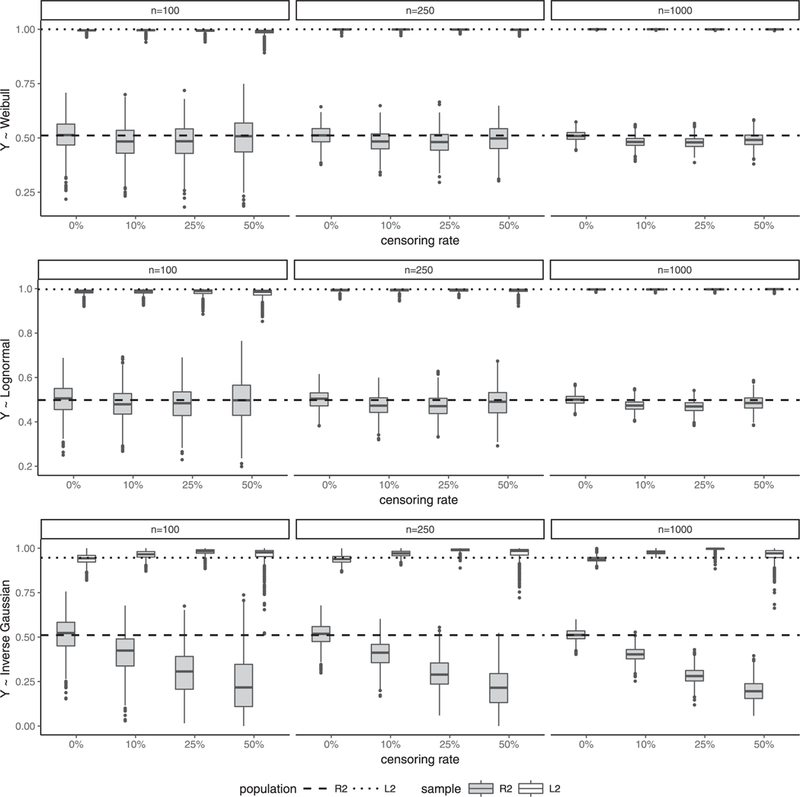
(Dependent censoring) Boxplots of simulated R² (shaded box) and L² (unshaded box) for the Cox model by censoring rate (0%, 10%, 25%, 50%), sample size (100,200,1000), and data generation setting (upper panel: Weibull; middle panel: log-normal AFT; bottom panel: inverse Gaussian).

5. An Example

In this section, we illustrate the use of the proposed prediction accuracy measures on a primary biliary cirrhosis (PBC) data with 312 patients from a randomized Mayo Clinic trial in primary biliary cirrhosis of the liver conducted between 1974 and 1984 (http://astrostatistics.psu.edu/datasets/R/html/survival/html/pbc.html). For illustration purpose, we evaluate and compare the predictive power of the Cox model, the Weibull and log-normal accelerated failure time models, and the threshold regression model for predicting overall survival of individual patients with PBC, using the five covariates (patient’s age, log(serum bilirubin concentration), log(serum albumin concentration), log(standardised blood clotting time), and presence of peripheral edema and antidiuretic therapy) employed in the well-known Mayo risk score (MRS) (Dickson et al. 1989).

We first examine the Cox-Snell residual plot based on the PBC data for each of the four predictions models in Figure 5 for overall lack-of-fit. In each plot, we have also overlaid additional Cox-Snell residual plots from 10 bootstrap samples to reflect the variability. Figure 5 does not indicate any serious lack-of-fit for the Cox model, Weibull and log-normal accelerated failure time models. However, it does suggest possible severe lack-of-fit for the threshold regression model, which is thus excluded from further consideration.

Figure 5.

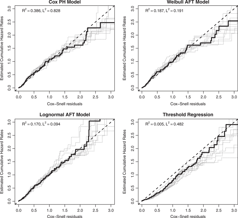
(PBCdata) Cox-Snell residual plots for the Cox model, Weibull AFT model, log-normal AFT model, and threshold regression model. For each model, the solid line is based on the observed PBC data and the dotted lines are based on 10 bootstrap samples. Deviations from the 45° line indicate possible lack-of-fit to the data.

Note that Figure 5 only provides a model diagnostic check for lack-of-fit. It does not offer further information regarding the predictive powers of the models under consideration especially because it is difficult to interpret the right tail of a Cox-Snell plot. In fact, plots of the predicted and observed survival times versus the risk scores for the three models in Figure 6 reveal that the Weibull AFT model and the log-normal AFT model could suffer substantial systematic prediction bias for low-risk patients (or long survivors). To assess and compare their predictive powers, we report their R² and L² values in Table 2.

Figure 6.

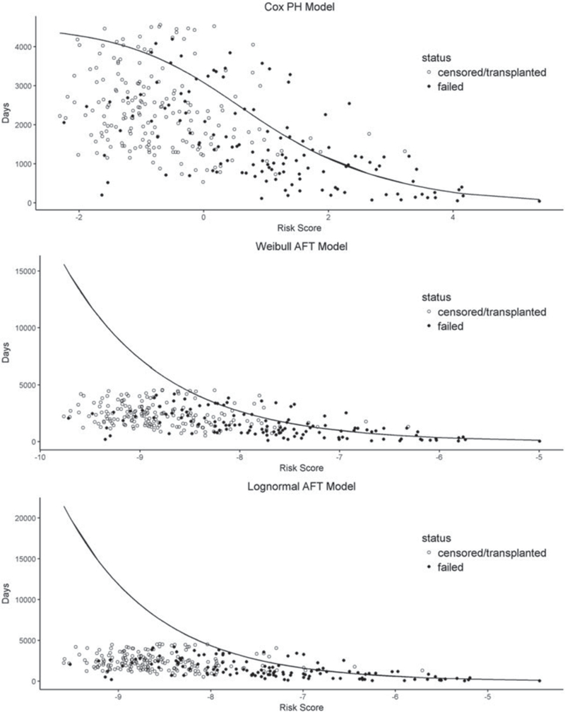
(PBC data) Predicted (solid line) and observed (solid dot: uncensored; censored: circle) survival times (in days) versus risk score for the Cox model (top panel), Weibull AFT model (middle panel), and log-normal AFT model (bottom panel).

Table 2.

(PBC data) R² values of different survival regression models.

Model	Cox PH model	Weibull AFT model	Log-normal AFT model
R2	0.39	0.19	0.17
L2	0.83	0.19	0.09

It is seen from Table 2 that among the three models, the Cox model stands out as the best prediction model with the highest potential predictive power R² = 0.39, which is consistent with the observation from Figure 6. To account for sampling variabilities, we also computed R² values for the three models based on 100 bootstrap samples and summarized the R² differences between the Cox model and each of the other two models using boxplots in Figure 7, which confirms the superior potential predictive power of the Cox model to the Weibull and lognormal AFT models. Finally, the Cox model has an associated L² value of 0.83, suggesting that a linear correction would be needed to fulfill its potential predictive power and that the linear correction would result in a reduction of 1 − L² = 17% of the mean squared prediction error.

Figure 7.

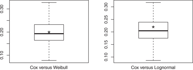
(PBC data) Boxplots of the R² differences between different models based on 100 bootstrap samples from the PBC data (Left: Cox’s model versus Log-normal AFT model; Right: Cox’s model versus Weibull AFT model). The asterisk in each boxplot represents the R² difference between the two models based on the observed PBC data.

6. Discussion

To assess the prediction accuracy of a nonlinear prediction function with right-censored data, we have first proposed a pair of population prediction accuracy parameters ρ² and λ² and then developed their sample versions R² and L² for both uncensored and censored data. The R² statistic, defined as the proportion of explained variance by its linearly corrected prediction function, quantifies the potential predictive power of the prediction function. The L² statistic, defined as the proportion of explained prediction error by its corrected prediction function, measures how close the prediction function is to its corrected prediction. Together, they give a complete summary regarding the prediction accuracy of a nonlinear prediction function. We highlight that the proposed R² statistic for right-censored data enjoys an appealing property that it educes to the classical coefficient of determination R² for the linear model in the absence of censoring, which is not shared by any other existing pseudo R² proposals for right-censored data. Furthermore, L² degenerates to 1 for the linear model with uncensored data. In practice, we recommend that R² be used as the primary measure to evaluate and compare the potential predictive power between competing prediction models, and L² be used as a supplementary measure only for the final prediction model of interest (such as the one with the largest R² value) to indicate by a value less 1 if a correction is needed for the prediction function to fulfill its potential predictive power and quantify how much prediction error reduction can be realized by the correction, as illustrated in the real data example in Section 5.

Our simulation results show that the sample R² and L² measures estimate their corresponding population parameters well with little bias with moderate sample size and censoring rate, regardless of whether the model is correctly or misspecified. The consistency of the proposed measures for right-censored data is derived under a rather strong technical assumption that the censoring time is independent of both the survival time and the covariates. However, our simulation results indicate that even when the independent censoring assumption is violated, the proposed measures still estimate their population counterparts well, except when the model is severely misspecified. Therefore, in the presence of dependent censoring, it is important to routinely perform model diagnostics to identify and eliminate a severely misspecified model before further applying the proposed measures to evaluate its prediction power. Finally, L² = 1 simply indicates that no correction is needed for the prediction function to achieve its potential prediction power. It should not be used to suggest a good fit of the model to the data as discussed in Remark 2.1.

This article focuses on event time models with a single failure type, time-independent covariates and independently right-censored data. Future efforts to develop prediction accuracy measures for event time models with time-dependent covariates, competing risks, time-varying effects, and other censoring patterns are warranted. It would also be interesting to extend the proposed measures to weighted R² and L² that naturally follow from some weighted versions of the variance and prediction error decompositions similar to Lemma A.3, which could be useful to evaluate the local predictive performance for some subpopulation of interest. Our team is also investigating the application of the proposed R² measure for node-splitting in survival tree regression and survival random forest.

References

- Ash A, and Shwartz M (1999), “R2: A Useful Measure of Model Performance When Predicting a Dichotomous Outcome,” Statistics in Medicine, 18, 375–384. [1] [DOI] [PubMed] [Google Scholar]
- Cox DR (1972), “Regression Models and Life Tables” (with discussion), Journal of the Royal Statistical Society, Series B, 34, 187–220. [2] [Google Scholar]
- Cox DR, and Snell EJ (1989), Analysis of Binary Data (Vol. 32), New York: CRC Press; [1] [Google Scholar]
- Cox DR, and Wermuth N (1992), “A Comment on the Coefficient of Determination for Binary Responses,” The American Statistician, 46, 1–4. [1] [Google Scholar]
- Dickson ER, Grambsch PM, Fleming TR, Fisher LD, and Langworthy A (1989), “Prognosis in Primary Biliary Cirrhosis: Model for Decision Making,” Hepatology, 10, 1–7. [8] [DOI] [PubMed] [Google Scholar]
- Efron B (1978), “Regression and ANOVA with Zero-One Data: Measures of Residual Variation,” Journal of the American Statistical Association, 73, 113–121. [1] [Google Scholar]
- Efron B, and Tibshirani RJ (1994), An Introduction to the Bootstrap, New York: CRC Press; [4] [Google Scholar]
- Goodman LA (1971), “The Analysis of Multidimensional Contingency Tables: Stepwise Procedures and Direct Estimation Methods for Building Models for Multiple Classifications,” Technometrics, 13, 33–61. [1] [Google Scholar]
- Graf E, Schmoor C, Sauerbrei W, and Schumacher M (1999), “Assessment and Comparison of Prognostic Classification Schemes for Survival Data,” Statistics in Medicine, 18, 2529–2545. [2] [DOI] [PubMed] [Google Scholar]
- Haberman SJ (1982), “Analysis of Dispersion of Multinomial Responses,” Journal of the American Statistical Association, 77, 568–580. [1] [Google Scholar]
- Harrell FE, Califf RM, Pryor DB, Lee KL, and Rosati RA (1982), “Evaluating the Yield of Medical Tests,” JAMA, 247, 2543–2546. [1] [PubMed] [Google Scholar]
- Hilden J (1991), “The Area Under the ROC Curve and its Competitors,” Medical Decision Making, 11, 95–101. [1] [DOI] [PubMed] [Google Scholar]
- Kaplan E, and Meier P (1958), “Nonparametric Estimation From Incomplete Observations,” Journal of the American Statistical Association, 53, 457–481. [5] [Google Scholar]
- Kent JT (1983), “Information Gain and a General Measure of Correlation,” Biometrika, 70, 163–173. [1] [Google Scholar]
- Kent JT, and O’Quigley J (1988), “Measures of Dependence for Censored Survival Data,” Biometrika, 75, 525–534. [2] [Google Scholar]
- Korn EL, and Simon R (1990), “Measures of Explained Variation for Survival Data,” Statistics in Medicine, 9, 487–503. [2] [DOI] [PubMed] [Google Scholar]
- Lee M-LT, and Whitmore GA (2006), “Threshold Regression for Survival Analysis: Modeling Event Times by a Stochastic Process Reaching a Boundary,” Statistical Science, 21, 501–513. [6] [Google Scholar]
- Maddala GS (1986), Limited-Dependent and Qualitative Variables in Econometrics (No. 3). New York: Cambridge University Press; [1] [Google Scholar]
- Magee L (1990), “R2 Measures Based on Wald and Likelihood Ratio Joint Significance Tests,” The American Statistician, 44, 250–253. [1] [Google Scholar]
- McFadden D (1973), “Conditional Logit Analysis of Qualitative Choice Behavior,” in Frontiers in Econometrics, ed. Zarembka P, New York: Wiley; [1] [Google Scholar]
- Mittlbock M, and Schemper M, (1996), “Explained Variation for Logistic Regression,” Statistics in Medicine, 15, 1987–1997. [1] [DOI] [PubMed] [Google Scholar]
- Nagelkerke NJ (1991), “A Note on a General Definition of the Coefficient of Determination,” Biometrika, 78, 691–692. [1] [Google Scholar]
- O’Quigley J, Xu R, and Stare J (2005), “Explained Randomness in Proportional Hazards Models,” Statistics in Medicine, 24, 479–489. [2] [DOI] [PubMed] [Google Scholar]
- Rényi A (1959), “On Measures of Dependence,” Acta Mathematica Hungarica, 10,441–451. [4] [Google Scholar]
- Royston P, and Sauerbrei W (2004), “A New Measure of Prognostic Separation in Survival Data,” Statistics in Medicine, 23, 723–748. [2] [DOI] [PubMed] [Google Scholar]
- Schemper M and Henderson R (2000), “Predictive Accuracy and Explained Variation in Cox Regression,” Biometrics, 56, 249–255. [2,5] [DOI] [PubMed] [Google Scholar]
- Stare J, Perme MP, and Henderson R (2011), “ Measure of Explained Variation for Event History Data,” Biometrics, 67, 750–759. [2,5] [DOI] [PubMed] [Google Scholar]
- Theil H (1970), “On the Estimation of Relationships Involving Qualitative Variables,” American Journal of Sociology, 76, 103–154. [1] [Google Scholar]
- Zheng B, and Agresti A (2000), “Summarizing the Predictive Power of a Generalized Linear Model,” Statistics in Medicine, 19, 1771–1781. [1] [DOI] [PubMed] [Google Scholar]
Associated Data
This section collects any data citations, data availability statements, or supplementary materials included in this article.