Dynamics identification and forecasting of COVID-19 by switching Kalman filters

Abstract

The COVID-19 pandemic has captivated scientific activity since its early days. Particular attention has been dedicated to the identification of underlying dynamics and prediction of future trend. In this work, a switching Kalman filter formalism is applied on dynamics learning and forecasting of the daily new cases of COVID-19. The main feature of this dynamical system is its ability to switch between different linear Gaussian models based on the observations and specified probabilities of transitions between these models. It is thus able to handle the problem of hidden state estimation and forecasting for models with non-Gaussian and nonlinear effects. The potential of this method is explored on the daily new cases of COVID-19 both at the state-level and the country-level in the US. The results suggest a common disease dynamics across states that share certain features. We also demonstrate the ability to make short to medium term predictions with quantifiable error bounds.

Introduction

The pandemic of COVID-19, also known as SARS-CoV-2, has already caused several hundreds of thousands deaths worldwide while bringing the global economy to a standstill. The long incubation period, large portion of asymptomatic infections, highly contagious rate, testing accuracy problem in the early stages of the spread, and the difficulty to implement uniform nationwide policies, are just some of the challenges in containing the spread of the virus. In the meantime, relatively long-duration treatment and high death rate have overwhelmed public health systems. Capturing the underlying disease dynamics with the ability for credible statistical predictions is ever so critical for health care providers and decision makers to be better prepared through resource allocation to ultimately contain the virus.

Modeling and forecasting of COVID-19 cases have recently received large attention. The fundamental epidemic model, proposed in 1927 [1], is able to describe the dynamics of three population groups, namely, susceptible (S), infected (I), and recovered (R). The SIR family of models are among the most popular ones to learn the dynamics of COVID-19. Toda [2] used SIR model to study the effects of transmission rate to the growth of new cases, the economic impacts of the pandemic was also investigated. The SIRD model (“D” stands for “death”) is an extension of the SIR model, and is used by [3] to demonstrate the differences of infectious rate at different countries. Sarkar et al. [4] separated the susceptible individuals into unaffected and quarantined ones, and the infected individuals into asymptomatic and symptomatic ones, the modified SIR model was used to study the consequences of the public policies. He et al. [5] proposed a modified SEIR model (“E” stands for “exposed”) to adapt the particularities of COVID-19, which considers the social and government interventions, quarantine and treatment. To quantify the effectiveness of public health interventions (that change with time), Linda et al. [6] proposed a dynamic SEIR model with time-varying reproduction number. Radulescu and Cavanagh suggested to use separate SEIR models for different age compartments since they have different infection, recovery, and fatality parameters, and this model was applied to a small “college town” community to study the effects of several social interventions to the spread of the disease. Besides the SIR family models, there are also some other types of models that try to address the modeling and forecasting of COVID-19, including the phenomenological models [7], exponential smoothing models [8], autoregressive moving average and Wavelet-based models [9], artificial intelligence based models [10], time series models [11], and many others [12, 13].

The focus of the present work is to uncover some persistent dynamics within the daily new case data and make reasonable and reliable predictions of the future infections of the whole United States (US) as well as of individual states within the US. We explore the suitability of the switching Kalman filter (SKF) [14] algorithm as a viable tool for this purpose. Kalman filter (KF) is a widely used method for tracking and navigation, and for filtering and prediction of econometric time series [15]. The KF is efficient, and accurate, only when the hidden state is a linear Gaussian model, which is usually not true for most practical applications. By using a mixture of several linear Gaussian models, the SKF, however, is able to accurately estimate the hidden state that is governed by nonlinear and non-Gaussian dynamics [16–18]. More specifically, a weighted combination of linear models is used to estimate the true state at each time step. An addition hidden switching variables are introduced to specify which model to choose at any specific time step. The switching between models usually indicates a change in the underlying dynamics of the hidden state and hence is useful to monitor abnormal behavior in a system. It has been used, for instance, to monitor anomaly detection of dams [19], the diagnostics and prognostics of vehicle health [20], and the monitoring of bearing systems [21].

COVID-19 data used in this paper was extracted from [22]. The daily new case of the US is shown in Fig. 1, from which we can see that the time series can be split into several stages along the time, namely, the low-level new infections stage, the rapid increasing stage starting from March 1, the slow decreasing stage from the beginning of April to June 15, and another rapid increasing stage after that. By the clear separation of the data, we have reason to believe that there might be different dynamics driving the evolution of each stage. In addition, with the evolution of the spread of the virus, the communities change their personal attitude towards handling the disease and decision makers should make corresponding adjustments to their public policies. These factors can, in turn, drive changes in the dynamics of new infections. The SKF, with its ability to switch between dynamical systems, is well-adapted to these challenges.

Fig. 1.

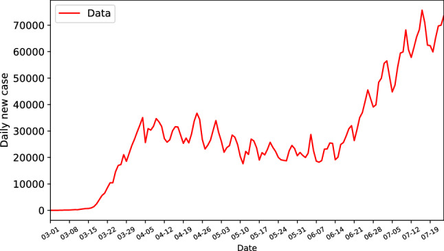
Daily new cases of the US up to July 24

The paper is organized as follows. Section 2 introduces the mathematical foundations of SKF, as well the ideas of learning its parameters from the observations. In Sect. 3, the models being used in SKF are introduced, including both the trend and seasonal models, the methodologies are also summarized into two algorithms. The numerical analyses of SKF on the actual data of the daily cases of the US and several states of the US are carried out in Sect. 4. In Sect. 5, we present the concluding remarks and discussions.

Switching Kalman filters

The mathematical foundation of SKF is presented in this section. The KF is first recalled, based on which the SKF method is introduced.

Kalman filter

The KF uses a linear state-space model to estimate the true (hidden) states, including past, present and future states, of a process from a set of observations, in which the mean squared error is minimized [23]. Denote ${\mathit{x}}_t\in {\mathbb{R}}^n$ the true state and ${\mathit{y}}_t\in {\mathbb{R}}^m$ the observation, the linear dynamic model that the KF tries to address can be specified as follows,

$$\begin{array}{c}\hfill \begin{array}{cc}\hfill {\mathit{x}}_t=& \mathit{A}{\mathit{x}}_{t-1}+{\mathit{w}}_t,\hfill \\ \hfill {\mathit{y}}_t=& {\mathit{Hx}}_t+{\mathit{v}}_t,\hfill \end{array}\end{array}$$ 1

where ${\mathit{w}}_t\sim \mathcal{N}(\mathbf{0},\mathit{Q})$, and ${\mathit{v}}_t\sim \mathcal{N}(\mathbf{0},\mathit{R})$ are the state and observation error matrices, respectively; $\mathit{A}$ ($n\times n$) and $\mathit{H}$ ($m\times n$) are the state transition and observation matrices, respectively. Note that, $\mathit{A}$, $\mathit{H}$, $\mathit{Q}$, and $\mathit{R}$ might change with time, but are assumed to be constant in this paper. In KF, $({\mathit{x}}_t|{\mathit{x}}_{t-1})$ and $({\mathit{y}}_t|{\mathit{x}}_t)$ are both assumed to be Gaussians. The KF consists of two steps, namely, a “prediction” step and an “updating” step [24]. Let ${\widehat{\mathit{x}}}_{t|t-1}$ be the prior estimate at time t given information available at time $t-1$, ${\mathit{V}}_{t|t-1}$ be the prior estimate of state error covariance, ${\widehat{\mathit{x}}}_t$ be the posterior estimate given observation ${\mathit{y}}_t$, and ${\mathit{V}}_t$ be the posterior estimate of the state error covariance. The KF process can then be expressed as,

KF prediction

$$\begin{array}{c}\hfill \begin{array}{cc}\hfill {\widehat{\mathit{x}}}_{t|t-1}& =\mathit{A}{\widehat{\mathit{x}}}_{t-1},\hfill \\ \hfill {\mathit{V}}_{t|t-1}& ={\mathit{AV}}_{t-1}{\mathit{A}}^T+\mathit{Q}.\hfill \end{array}\end{array}$$ 2

KF updating

$$\begin{array}{c}\hfill \begin{array}{cc}\hfill {\widehat{\mathit{x}}}_t& ={\widehat{\mathit{x}}}_{t|t-1}+{\mathit{K}}_t{\mathit{\nu }}_t,\hfill \\ \hfill {\mathit{V}}_t& =\left(\mathit{I},-,{\mathit{K}}_t,\mathit{H}\right){\mathit{V}}_{t|t-1},\hfill \end{array}\end{array}$$ 3

where ${\mathit{K}}_t={\mathit{V}}_{t|t-1}{\mathit{H}}^T{\left({\mathit{HV}}_{t|t-1},{\mathit{H}}^T,+,\mathit{R}\right)}^{-1}$ is referred to as the Kalman gain and ${\mathit{\nu }}_t={\mathit{y}}_t-\mathit{H}{\widehat{\mathit{x}}}_{t|t-1}$ is the so-called innovation process. The likelihood of observation ${\mathit{y}}_t$ given the observations of ${\mathit{y}}_{1:t-1}$ can also be obtained as a by-product of the process as

$$\begin{array}{c}\hfill L_t=p({\mathit{y}}_t|{\mathit{y}}_{1:t-1})=\mathcal{N}\left({\mathit{\nu }}_t,;,\mathbf{0},,,{\mathit{HV}}_{t|t-1},{\mathit{H}}^{\mathit{T}},+,\mathit{R}\right).\end{array}$$ 4

For further short-hand reference, the KF process containing the operations from Eqs. (2)–(4) is summarized as a subroutine of the form,

$$\begin{array}{c}\hfill [{\widehat{\mathit{x}}}_t,{\mathit{V}}_t,L_t]=\mathbf{Filter}\left({\widehat{\mathit{x}}}_{t-1},,,{\mathit{V}}_{t-1},,,{\mathit{y}}_t,,,\mathit{A},,,\mathit{Q},,,\mathit{H},,,\mathit{R}\right).\end{array}$$ 5

Kalman filter has been demonstrated in a wide range of applications from the navigation and tracking of vehicles and aircraft [24–26] to estimation and forecast in economics [27]. From the above analysis one can see that the KF uses a linear Gaussian dynamic model to estimate the hidden states of the processes. This is exact only when the underlying dynamical process is actually linear and the errors are Gaussian. However, the estimates by KF could be unsatisfactory for processes that are governed by nonlinear dynamics or where the errors are shaped by non-Gaussian effects.

Collapse and switching Kalman filters

Instead of using single linear Gaussian model, the SKF estimates the dynamical process as a mixture of N (with $N>1$) linear Gaussian models [14]. By construction, SKF is better able to estimate the hidden states of processes with nonlinear and non-Gaussian underlying dynamics, which is usually the case in practical applications.

An additional Markov “switching” variable $S_t$ with a model transition matrix $\mathit{Z}$ $(N\times N)$ is introduced in SKF to determine the weights of the linear models that are used at time t. Suppose that $S_t$ is known, the state at t is then estimated by a weighted combination of linear Gaussian models where the weight of each model is given by $\text{Pr}(S_t=i|{\mathit{y}}_{1:t})$, for $i=1,\dots ,N$. Assume that the initial state $p({\mathit{x}}_1)$ is a mixture of N Gaussians, and each Gaussian can be propagated forward by N different models, so that the belief state of $p({\mathit{x}}_2)$ will be a mixture of $N^2$ Gaussians. Then the state at t, $p({\mathit{x}}_t|{\mathit{y}}_{1:t})$, will be a mixture of $N^t$ Gaussians. That is, the size of the belief state grows exponentially with time, which makes the SKF system based on exact propagation of the state intractable. There are several approaches to deal with the exponential growth, in this paper we will focus on the Generalized Pseudo Bayesian (GPB) algorithm [14, 28]. In this algorithm, we estimate the state at any time by a fixed number of N Gaussians, which requires one to approximate a mixture of $N^t$ Gaussians at time t by a mixture of N Gaussians. This is achieved by a “collapsing” step which collapses a mixture of N Gaussians into a single one by first and second moments matching. Suppose that there is a mixture of Gaussians with mean values of ${\mathit{x}}^j$, covariances of ${\mathit{V}}^j$, and weights of $W^j$, for $j=1,2,\dots$, then the collapsing can be obtained as

$$\begin{array}{c}\hfill \begin{array}{cc}\hfill \mathit{x}& =\sum _j{W}^j{\mathit{x}}^j,\hfill \\ \hfill \mathit{V}& =\sum _j{W}^j\left[{\mathit{V}}^j,+,({\mathit{x}}^j-\mathit{x}),{({\mathit{x}}^j-\mathit{x})}^T\right].\hfill \end{array}\end{array}$$ 6

For further reference, the collapse step that contains the operation of Eq. (6) can be written as a subroutine as

$$\begin{array}{c}\hfill [\mathit{x},\mathit{V}]=\mathbf{Collapse}\left({\{{\mathit{x}}^j,{\mathit{V}}^j,W^j\}}_j\right).\end{array}$$ 7

Now, for the propagation from time $t-1$ to t, we can split the SKF process into two steps. Suppose that the posterior distribution $p({\mathit{x}}_{t-1}|{\mathit{y}}_{1:t-1})$ at time $t-1$ is a mixture of N Gaussians that is

$$\begin{array}{c}\hfill p({\mathit{x}}_{t-1}|{\mathit{y}}_{1:t-1},S_{t-1}=i)=\mathcal{N}\left({\mathit{x}}_{t-1}^i,,,{\mathit{V}}_{t-1}^i\right),\end{array}$$ 8

where the mean ${\mathit{x}}_{t-1}^i=\mathbb{E}[{\mathit{x}}_{t-1}|{\mathit{y}}_{1:t-1},S_{t-1}=i]$ and covariance ${\mathit{V}}_{t-1}^i=\text{Cov}[{\mathit{x}}_{t-1}|{\mathit{y}}_{1:t-1},S_{t-1}=i]$, for $i=1,\dots ,N$. The weight of Gaussian model i is obtained by $W_{t-1}^i=\text{Pr}(S_{t-1}=i|{\mathit{y}}_{1:t-1})$. Then the propagation from time $t-1$ to time t and from Gaussian model i to j is a KF, hence

$$\begin{array}{c}\hfill p({\mathit{x}}_t|{\mathit{y}}_{1:t},S_t=j,S_{t-1}=i)=\mathcal{N}\left({\mathit{x}}_t^{\mathit{ij}},,,{\mathit{V}}_t^{\mathit{ij}}\right),\end{array}$$ 9

where the mean ${\mathit{x}}_t^{\mathit{ij}}=\mathbb{E}[{\mathit{x}}_t|{\mathit{y}}_{1:t},S_t=j,S_{t-1}=i]$ and covariance ${\mathit{V}}_t^{\mathit{ij}}=\text{Cov}[{\mathit{x}}_t|{\mathit{y}}_{1:t},S_t=j,S_{t-1}=i]$. The first step of the propagation is then to use the Filter subroutine [Eq. (5)] to obtain ${\mathit{x}}_t^{\mathit{ij}}$ and ${\mathit{V}}_t^{\mathit{ij}}$ as

$$\begin{array}{c}\hfill \left[{\mathit{x}}_t^{\mathit{ij}},,,{\mathit{V}}_t^{\mathit{ij}},,,L_t^{\mathit{ij}}\right]=\mathbf{Filter}\left({\mathit{x}}_{t-1}^i,,,{\mathit{V}}_{t-1}^i,,,{\mathit{y}}_t,,,{\mathit{A}}_j,,,{\mathit{Q}}_j,,,{\mathit{H}}_j,,,{\mathit{R}}_j\right),\\ \hfill \end{array}$$ 10

where $L_t^{\mathit{ij}}=P({\mathit{y}}_t|{\mathit{y}}_{1:t-1},S_t=j,S_{t-1}=i)$ is the likelihood of observing ${\mathit{y}}_t$; ${\mathit{A}}_j$, ${\mathit{Q}}_j$, ${\mathit{H}}_j$, and ${\mathit{R}}_j$ are the state space matrices of Gaussian model j, for $j=1,\dots ,N$. The following by-products are also computed

$$\begin{array}{c}\hfill \begin{array}{cc}\hfill W_t^{\mathit{ij}}& =\text{Pr}(S_t=j,S_{t-1}=i|{\mathit{y}}_{1:t})=\frac{L_t^{\mathit{ij}}{Z}_{\mathit{ij}}{W}_{t-1}^i}{{\sum }_{i,j}{L}_t^{\mathit{ij}}{Z}_{\mathit{ij}}{W}_{t-1}^i},\hfill \\ \hfill W_t^j& =\text{Pr}(S_t=j|{\mathit{y}}_{1:t})=\sum _i{W}_t^{\mathit{ij}},\hfill \\ \hfill M_t^{\mathit{ij}}& =\text{Pr}(S_{t-1}=i|S_t=j,{\mathit{y}}_{1:t})=\frac{W_t^{\mathit{ij}}}{W_t^j},\hfill \end{array}\end{array}$$ 11

where $Z_{\mathit{ij}}=\text{Pr}\left(S_t,=j|,S_{t-1},=,i\right)$ is the component of the model transition matrix $\mathit{Z}$. Then the second step of the propagation is to collapse the mixture of $N^2$ Gaussians into a mixture of N Gaussians by the Collapse subroutine (7) as

$$\begin{array}{c}\hfill \left[{\mathit{x}}_t^j,,,{\mathit{V}}_t^j\right]=\mathbf{Collapse}\left({\{{\mathit{x}}_t^{\mathit{ij}},{\mathit{V}}_t^{\mathit{ij}},M_t^{\mathit{ij}}\}}_i\right).\end{array}$$ 12

When a single estimate of the state is desired, the Collapse subroutine can be applied again on the N mixture of Gaussians and obtain a single Gaussian distribution.

The model parameters, for instance $\mathit{A}$, $\mathit{H}$, $\mathit{Q}$, and $\mathit{R}$, remain to be estimated from the available information. In practice, the hidden state ${\mathit{x}}_{1:t}$ is usually hard to obtain, hence, only the observation data ${\mathit{y}}_{1:t}$ is provided for parameter estimation. The method of maximum likelihood estimator (MLE) [29] is utilized for such purpose, in which the log-likelihood of the observation is first obtained as

$$\begin{array}{cc}\hfill ln\left({\mathit{y}}_{1:\tau }\right)& =ln\prod _{t}p\left({\mathit{y}}_t,|,{\mathit{y}}_{1:t-1}\right)\hfill \\ \hfill & =\sum _{t}lnp\left({\mathit{y}}_t,|,{\mathit{y}}_{1:t-1}\right)\hfill \\ \hfill & =\sum _{t}ln\left[\sum _{i,j=1}^N,p,\left({\mathit{y}}_t,,,S_t,=,j,,,S_{t-1},=i|,{\mathit{y}}_{1:t-1}\right)\right]\hfill \\ \hfill & =\sum _{t}ln\left[\sum _{i,j=1}^N,L_t^{\mathit{ij}},\text{Pr},\left(S_t,=,j,,,S_{t-1},=i|,{\mathit{y}}_{1:t-1}\right)\right]\hfill \\ \hfill & =\sum _{t}ln\left[\sum _{i,j=1}^N,L_t^{\mathit{ij}},Z_{\mathit{ij}},\text{Pr},\left(S_{t-1},=i|,{\mathit{y}}_{1:t-1}\right)\right]\hfill \\ \hfill & =\sum _{t}ln\left[\sum _{i,j=1}^N,L_t^{\mathit{ij}},Z_{\mathit{ij}},W_{t-1}^i\right].\hfill \end{array}$$ 13

In Eq. 13, $\tau$ is the end time of the data; and, $L_t^{\mathit{ij}}$, $Z_{\mathit{ij}}$ and $W_{t-1}^i$ are the same as in Eqs. (10) and (11). The set of parameters, denoted as $\mathcal{P}$, are embedded in the distribution of ${\mathit{y}}_{1:T}$ and can be estimated by maximizing the log-likelihood function as

$$\begin{array}{c}\hfill {\mathcal{P}}^{\ast }={\arg \max }_{\mathcal{P}}ln\left({\mathit{y}}_{1:t},|\mathcal{P}\right).\end{array}$$ 14

To avoid local maxima, the global optimization method, Basin-hopping [16], is used to solve Eq. (14).

Step-ahead predictor

The SKF follows the one-step prediction and updating algorithm, hence, the observation at time $t+1$ is required for the hidden state estimation at $t+1$. However, we are also interested in the step-ahead prediction without knowing the observations of the future. More specifically, the prediction of one step ahead (at time $t+1$) or several steps ahead (at time $t+r$) given that the state at time t is known. We start with the one-step-ahead predictor, in which, $p({\mathit{x}}_{t+1}|{\mathit{x}}_t)$ is first computed as

$$\begin{array}{c}\hfill \begin{array}{cc}\hfill p({\mathit{x}}_{t+1}|{\mathit{x}}_t)=& \sum _{i,j=1}^{N}p({\mathit{x}}_{t+1},S_{t+1}=j,S_t=i|{\mathit{x}}_t)\hfill \\ \hfill =& \sum _{i,j=1}^{N}p({\mathit{x}}_{t+1}|{\mathit{x}}_t,S_{t+1}=j,S_t=i)·\hfill \\ \hfill & \text{Pr}(S_{t+1}=j,S_t=i|{\mathit{x}}_t)\hfill \\ \hfill =& \sum _{i,j=1}^{N}p({\mathit{x}}_{t+1}|{\mathit{x}}_t,S_{t+1}=j,S_t=i)W_{t+1|t}^{\mathit{ij}},\hfill \end{array}\end{array}$$ 15

where $W_{t+1|t}^{\mathit{ij}}=\text{Pr}(S_{t+1}=j,S_t=i|{\mathit{x}}_t)=W_{t+1|t}^j{M}_{t+1|t}^{\mathit{ij}}$, where $W_{t+1|t}^j=P(S_{t+1}=j|{\mathit{x}}_t)$ and $M_{t+1|t}^{\mathit{ij}}=\text{Pr}(S_t=i|S_{t+1}=j,{\mathit{x}}_t)$. Please note the differences of definitions between $W_{t+1|t}^{\mathit{ij}}$ and $W_t^{\mathit{ij}}$, $W_{t+1|t}^j$ and $W_t^j$, and $M_{t+1|t}^{\mathit{ij}}$ and $M_t^{\mathit{ij}}$. By assumptions of KF, we have

$$\begin{array}{c}\hfill P({\mathit{x}}_{t+1}|{\mathit{x}}_t,S_{t+1}=j,S_t=i)=\mathcal{N}\left({\mathit{x}}_{t+1|t}^{\mathit{ij}},,,{\mathit{V}}_{t+1|t}^{\mathit{ij}}\right),\end{array}$$ 16

where the mean ${\mathit{x}}_{t+1|t}^{\mathit{ij}}=\mathbb{E}\left[{\mathit{x}}_{t+1},|,{\mathit{x}}_t,,,S_{t+1},=,j,,,S_t,=,i\right]$ and the covariance ${\mathit{V}}_{t+1|t}^{\mathit{ij}}=\text{Cov}\left[{\mathit{x}}_{t+1},|,{\mathit{x}}_t,,,S_{t+1},=,j,,,S_t,=,i\right]$. Then, similar to Eq. (11) we can compute

$$\begin{array}{c}\hfill \begin{array}{cc}\hfill W_{t+1|t}^{\mathit{ij}}& =\frac{Z_{\mathit{ij}}{W}_{t|t-1}^i}{{\sum }_{i,j}{Z}_{\mathit{ij}}{W}_{t|t-1}^i},\hfill \\ \hfill W_{t+1|t}^j& =\sum _i{W}_{t+1|t}^{\mathit{ij}},\hfill \\ \hfill M_{t+1|t}^{\mathit{ij}}& =\frac{W_{t+1|t}^{\mathit{ij}}}{W_{t+1|t}^j}.\hfill \end{array}\end{array}$$ 17

Note that, different from Eqs. (11), (17) does not have the likelihood function of the observation since the observation at time $t+1$ is not available. Moreover, Eq. (17) is a recursive form, the initial condition of which, suppose that the step-ahead predictor starts with time t, is $W_{t|t-1}^i=W_t^i$ where $W_t^i$ is obtained from Eq. (11). We can see that the one-step-ahead predictor is a mixture of $N^2$ Gaussian. A Collapse step can be followed to reduce the number of mixture Gaussians to N. The step ahead propagation from time t to $t+1$ can also be split into two steps, with the first step being the predicting part of the Filter subroutine, that is

$$\begin{array}{c}\hfill \begin{array}{cc}\hfill {\mathit{x}}_{t+1|t}^{\mathit{ij}}=& {\mathit{A}}_j{\mathit{x}}_t^i,\hfill \\ \hfill {\mathit{V}}_{t+1|t}^{\mathit{ij}}=& {\mathit{A}}_j{\mathit{V}}_t^i{\mathit{A}}_j^T+{\mathit{Q}}_j.\hfill \\ \hfill \end{array}\end{array}$$ 18

In the second step, a collapse step is applied

$$\begin{array}{c}\hfill [{\mathit{x}}_{t+1}^j,{\mathit{V}}_{t+1}^j]=\mathbf{Collapse}\left({\{{\mathit{x}}_{t+1|t}^{\mathit{ij}},{\mathit{V}}_{t+1|t}^{\mathit{ij}},M_{t+1|t}^{\mathit{ij}}\}}_i\right).\end{array}$$ 19

From which we can see that the one-step-ahead predictor uses only the estimated state of the current step to predict the state of the next step. With the recursive manner, this predictor can be easily extended to a multi-step-ahead predictor by letting the predicted state of the current step be the available information for the next step prediction.

Models and methodology

Trend component

In the classical additive decomposition [30], the time series ${\mathit{x}}_t$ can be decomposed as

$$\begin{array}{c}\hfill {\mathit{x}}_t={\mathit{m}}_t+{\mathit{s}}_t+{\mathit{ϵ}}_t,\end{array}$$ 20

where ${\mathit{m}}_t$ is the slow changing trend component, ${\mathit{s}}_t$ is the seasonal component that has known period T, and ${\mathit{ϵ}}_t$ is the random noise component. One can relax the decomposition and obtain the trend plus noise model as

$$\begin{array}{c}\hfill {\mathit{x}}_t={\mathit{m}}_t+{\mathit{ϵ}}_t.\end{array}$$ 21

In time series analysis, the polynomial models have been widely applied to filtering and prediction since they can efficiently capture the trend component [31]. The 0th and 1th order polynomials are proved to be adequate for short term predictions. The COVID-19 data is affected by many factors including the population density, mobility of the community, temperature, testing credibility, masks policy, lock down policy, personal attitude, personal health predisposition, etc. With the high complexity, the 1th and 2nd order polynomials are used to predict the trend components. The 2nd order polynomials are useful for prediction problem with longer lead time [31], which is the case for COVID-19 data.

The model constructed by the 1th order polynomials in the state space is also known as the constant velocity model. The state vector is $\mathit{x}={[x,\dot{x}]}^T$, and the velocity is assumed to be constant over time, that is $\partial {\dot{\mathit{x}}}_t/\partial t=0$. The state transition and state error covariance matrices of the model can be obtained as [24]

$$\begin{array}{c}\hfill {\mathit{A}}_{\text{vel}}=\left[\begin{array}{cc}1& \Delta t\\ 0& 1\\ \end{array}\right],{\mathit{Q}}_{\text{vel}}={\sigma }_q^2\left[\begin{array}{cc}\frac{1}{3}\Delta t^3& \frac{1}{2}\Delta t^2\\ \frac{1}{2}\Delta t^2& \Delta t\\ \end{array}\right],\end{array}$$ 22

where $\Delta t$ is the sample interval, and ${\sigma }_q^2$ is a constant that defines the level of variance in the error.

The model constructed by the 2nd order polynomials in the state space is also known as the constant acceleration model. The state vector is $\mathit{x}={[x,\dot{x},\ddot{x}]}^T$, and the acceleration is assumed to be constant over time, that is $\partial {\ddot{\mathit{x}}}_t/\partial t=0$. The state transition and state error covariance matrices of the model can be obtained as [24]

$$\begin{array}{cc}\hfill {\mathit{A}}_{\text{acc}}=& \left[\begin{array}{ccc}1& \Delta t& \Delta t^2\\ 0& 1& \Delta t\\ 0& 0& 1\end{array}\right],\hfill \\ \hfill {\mathit{Q}}_{\text{acc}}=& {\sigma }_q^2\left[\begin{array}{ccc}\Delta t^5/20& \Delta t^4/8& \Delta t^3/6\\ \Delta t^4/8& \Delta t^3/3& \Delta t^2/2\\ \Delta t^3/3& \Delta t^2/2& \Delta t\\ \end{array}\right].\hfill \end{array}$$ 23

Seasonal component

By visually inspecting, the daily new cases data of the US in Fig. 1 exhibits a periodic behavior with the period approximately equals 7 days. In this paper, several seasonal components are used to capture the periodic behavior. Each of the seasonal component, ${\mathit{s}}_t^j$, is modeled by a harmonic function of sines and cosines recursively with a specified frequency $T_j$ as [32]

$$\begin{array}{c}\hfill \left(\begin{array}{c}{\mathit{s}}_t^j\\ {\mathit{s}}_t^{j\ast }\end{array}\right)=\left[\begin{array}{cc}cos{\omega }_j& sin{\omega }_j\\ -sin{\omega }_j& cos{\omega }_j\\ \end{array}\right]\left(\begin{array}{c}{\mathit{s}}_{t-1}^j\\ {\mathit{s}}_{t-1}^{j\ast }\end{array}\right)={\mathit{A}}_{{\mathit{s}}^j}\left(\begin{array}{c}{\mathit{s}}_{t-1}^j\\ {\mathit{s}}_{t-1}^{j\ast }\end{array}\right),\end{array}$$ 24

where ${\omega }_j=2\pi /T_j$ is the angular frequency. In Eq. (24), ${\mathit{s}}_t^j$ is the seasonal value at time t, and ${\mathit{s}}_t^{j\ast }$ is an auxiliary value by construction. The error covariance matrix associated with ${\mathit{s}}_t^j$ and ${\mathit{s}}_t^{j\ast }$ is given by

$$\begin{array}{c}\hfill {\mathit{Q}}_{{\mathit{s}}^j}=\left[\begin{array}{cc}{\sigma }_{{\mathit{s}}^j}^2& 0\\ 0& {\sigma }_{{\mathit{s}}^j}^2\end{array}\right],\end{array}$$ 25

where ${\sigma }_{{\mathit{s}}^j}^2$ is a constant.

Incorporating the trend components with the seasonal components, the state space matrices of the constant velocity model becomes

$$\begin{array}{c}\hfill \begin{array}{cc}\hfill \mathit{A}=& \text{blkdiag}\left({\mathit{A}}_{\text{vel}},,,,{\mathit{A}}_{{\mathit{s}}^1},,,,\dots ,,,,{\mathit{A}}_{{\mathit{s}}^{n_s}}\right),\hfill \\ \hfill \mathit{Q}=& \text{blkdiag}\left({\mathit{Q}}_{\text{vel}},,,,{\mathit{Q}}_{{\mathit{s}}^1},,,,\dots ,,,,{\mathit{Q}}_{{\mathit{s}}^{n_s}}\right),\hfill \\ \hfill \mathit{H}=& \left[\begin{array}{ccccccc}1,& 0,& 1,& 0,& \dots ,& 1,& 0,\end{array}\right],\hfill \\ \hfill \mathit{R}=& {\sigma }_r^2,\hfill \end{array}\end{array}$$ 26

where $n_s$ is the number of seasonal components; “blkdiag” denotes a block diagonalization operator. Similarly, the state space matrices of the constant acceleration model becomes

$$\begin{array}{c}\hfill \begin{array}{cc}\hfill \mathit{A}=& \text{blkdiag}\left({\mathit{A}}_{\text{acc}},,,,{\mathit{A}}_{{\mathit{s}}^1},,,,\dots ,,,,{\mathit{A}}_{{\mathit{s}}^{n_s}}\right),\hfill \\ \hfill \mathit{Q}=& \text{blkdiag}\left({\mathit{Q}}_{\text{acc}},,,,{\mathit{Q}}_{{\mathit{s}}^1},,,,\dots ,,,,{\mathit{Q}}_{{\mathit{s}}^{n_s}}\right),\hfill \\ \hfill \mathit{H}=& \left[\begin{array}{cccccccc}1,& 0,& 0,& 1,& 0,& \dots ,& 1,& 0,\end{array}\right],\hfill \\ \hfill \mathit{R}=& {\sigma }_r^2.\hfill \end{array}\end{array}$$ 27

For the COVID-19 data of the US, the cyclic behavior is clearly non-harmonic with additional fluctuations within each cycle. To better capture these dynamics, two seasonal components ($n_s=2$) with $T_1=7$ and $T_2=3.5$ days are incorporated.

Methodology

From the previous analysis, the set of unknown parameters that remains to be learned from the COVID-19 data is

$$\begin{array}{c}\hfill \mathcal{P}=\left({\sigma }_{q_{\text{acc}}}^2,,,{\sigma }_{q_{\text{vel}}}^2,,,{\sigma }_r^2,,,{\sigma }_{{\mathit{s}}^1}^2,,,{\sigma }_{{\mathit{s}}^2}^2\right).\end{array}$$ 28

The lower bound and upper bound for all the parameters are chosen to be $1.0\times {10}^{-7}$ and $1.0\times {10}^7$, that are large enough to be able to include the optimal solution. The model transition matrix is assumed to be

$$\begin{array}{c}\hfill \mathit{Z}=\left[\begin{array}{cc}{Z}_{11}& Z_{12}\\ Z_{21}& Z_{22}\end{array}\right]=\left[\begin{array}{cc}0.99& 0.01\\ 0.01& 0.99\end{array}\right].\end{array}$$ 29

That is, the state tends to remain on its own state. The choice of the transition matrix is based on the nature that the daily new cases data of COVID-19 usually has several stages, namely, the steady growth stage, super linearly growth stage, flat curve stage, and decreasing stage, and these stages remain for a period of time before it switches to the next trend, that is, it tends to remain on its own stage.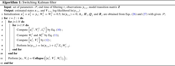

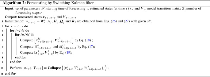
The SKF method and its multi-step-ahead predictor are summarized in Algorithms 1 and 2, respectively. For the purpose of dynamics learning of the COVID-19 data, the Basin-hopping optimization is first used to find the optimal set of parameters ${\mathcal{P}}^{\ast }$ by maximizing the log-likehood of the observations, $ln({\mathit{y}}_{1:\tau })$, that is obtained from Algorithm 1. In other words, Algorithm 1 serves as an objective function in the optimization problem. The data up to time $\tau$ is the training set and is defined by the user. After obtaining the optimal set of parameters ${\mathcal{P}}^{\ast }$, it can then be fed into Algorithm 1 again to estimate the hidden states ${\mathit{x}}_{1:\tau }$, where $\tau$ is the end time that the user intends to estimate. Note that the end time of the estimation can be different from the end time of the training set. These estimations can be compared with the data to verify the validity of the learned dynamics. Finally, for the purpose of forecasting of the COVID-19 data, in which no further observations are known beyond time $\tau$, Algorithm 2 can be used to perform multi-step-ahead predictions starting from $\tau$, with specified number of steps r. The r steps ahead predictions are used to approximate the future trend of the data. The forecasting can also start from any date of the available data, say ${\tau }^{\prime }$ with ${\tau }^{\prime }<\tau -r$, then the forecasts are obtained by assuming that the data after ${\tau }^{\prime }$ is not available. The r steps ahead predictions in this case can then be compared with the data to quantify the accuracy of the forecasts.

Dynamics learning and forecasting of the COVID-19 of the US

Dynamics learning and validation

In this section, the SKF is first used to identify the hidden dynamics behind the daily new cases of the COVID-19 of the US, including the whole US and some individual states, for instance, California (CA), New York (NY), Florida (FL), Texas (TX), North Carolina (NC), Georgia (GA) and Alabama (AL). The selected states are either the previous epicenter, or the ones that have rapid increasing trends currently based on the data up to July 24.

The incubation period of COVID-19 can be as long as 14 days according to [33], the infections from asymptomatic to symptomatic are postponed to be shown in the data. In addition, the wait time to get the test results is usually 3$\sim$5 days [34], and this time is extended with the number of people being tested increased rapidly starting in July. Thus, the severity of the pandemic today is only presented in the data after one week or so, which in turn causes the delays of social reactions. These delays can postpone the effects of policy interventions, including lock down, quarantine, mandated masks, mandated social distancing, etc. As a result, the time series of daily new cases has slow changing dynamics, even though the dynamics evolves with time. In other words, the dynamics of the next several days might not have large variation from the dynamics of the previous several days. This provides the foundation to do step-ahead predictions. Moreover, one might not need to use all the available data to capture the embedded dynamics as long as the additional data will not alter the current dynamics significantly.

To verify this, the Basin-hopping optimization and Algorithm 1 are used to learn the dynamics based on two different training sets, namely, the set with data up to June 30 and the set with data up to July 20. The optimal parameters for the US and several individual states are shown in Tables 1 and 2, the first three parameters of these two tables define the trend component. Note that the behavior of the KF is highly affected by the ratios of two error covariances [8, 35], ${\sigma }_{q_{\text{acc}}}^2/{\sigma }_r^2$ and ${\sigma }_{q_{\text{vel}}}^2/{\sigma }_r^2$. By comparing Tables 1 and 2 for the same locations, the error covariances of the observation, ${\sigma }_r^2$, only have minor differences. Though, the differences between ${\sigma }_{q_{\text{acc}}}^2$ and ${\sigma }_{q_{\text{vel}}}^2$ could be significant for some locations, for instance the US, CA and NC, the ratios of ${\sigma }_{q_{\text{acc}}}^2/{\sigma }_r^2$ and ${\sigma }_{q_{\text{vel}}}^2/{\sigma }_r^2$ remain at low levels. That means the dynamics learned from training data up to June 30 is similar to that learned from training data up to July 20.

Table 1.

Parameters learned from data up to July 20

Places	${\sigma }_{q_{\text{acc}}}^2$	${\sigma }_{q_{\text{vel}}}^2$	${\sigma }_r^2$	${\sigma }_{{\mathit{s}}^1}^2$	${\sigma }_{{\mathit{s}}^2}^2$
US	${10}^{4.0}$	${10}^{-2.1}$	${10}^{6.3}$	${10}^{5.0}$	${10}^{3.7}$
CA	${10}^{2.7}$	${10}^{2.0}$	${10}^{5.2}$	${10}^{3.7}$	${10}^{2.9}$
NY	${10}^{2.7}$	${10}^{-3.8}$	${10}^{5.8}$	${10}^{4.2}$	${10}^{-6.8}$
FL	${10}^{2.5}$	${10}^{1.5}$	${10}^{5.5}$	${10}^{4.0}$	${10}^{4.0}$
TX	${10}^{2.2}$	${10}^{-7.0}$	${10}^{5.3}$	${10}^{4.0}$	${10}^{2.5}$
NC	${10}^{1.3}$	${10}^{0.1}$	${10}^{4.3}$	${10}^{2.2}$	${10}^{-6.5}$
GA	${10}^{0.6}$	${10}^{1.1}$	${10}^{4.9}$	${10}^{2.6}$	${10}^{2.8}$
AL	${10}^{-1.5}$	${10}^{0.1}$	${10}^{4.5}$	${10}^{1.6}$	${10}^{1.3}$

Table 2.

Parameters learned from data up to June 30

Places	${\sigma }_{q_{\text{acc}}}^2$	${\sigma }_{q_{\text{vel}}}^2$	${\sigma }_r^2$	${\sigma }_{{\mathit{s}}^1}^2$	${\sigma }_{{\mathit{s}}^2}^2$
US	${10}^{3.3}$	${10}^{3.2}$	${10}^{6.3}$	${10}^{4.9}$	${10}^{3.8}$
CA	${10}^{1.2}$	${10}^{1.8}$	${10}^{5.0}$	${10}^{3.9}$	${10}^{2.4}$
NY	${10}^{2.8}$	${10}^{-2.8}$	${10}^{5.8}$	${10}^{4.2}$	${10}^{-4.9}$
FL	${10}^{1.3}$	${10}^{1.8}$	${10}^{4.8}$	${10}^{4.3}$	${10}^{3.0}$
TX	${10}^{1.9}$	${10}^{1.3}$	${10}^{4.8}$	${10}^{3.0}$	${10}^{3.0}$
NC	${10}^{-2.0}$	${10}^{0.5}$	${10}^{4.1}$	${10}^{2.4}$	${10}^{-5.0}$
GA	${10}^{-0.1}$	${10}^{1.5}$	${10}^{4.5}$	${10}^{2.7}$	${10}^{2.6}$
AL	${10}^{-2.2}$	${10}^{0.5}$	${10}^{4.4}$	${10}^{-5.5}$	${10}^{0.4}$

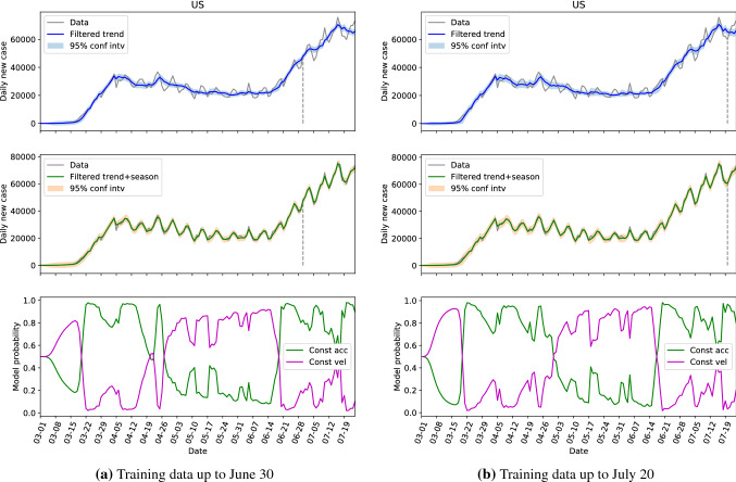
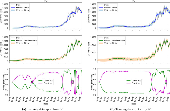
Graphically, the comparisons of the hidden state estimations given by Algorithm 1 with parameters learned from two different training sets of two representative locations, the US and Florida, are presented in Figs. 2 and 3. In these figures, the top ones present the filtered (or estimated) trend components with 95% confidence intervals, the middle ones show the filtered trend plus seasonal components with 95% confidence intervals, and the bottom one depicts the probabilities of the constant acceleration and constant velocity models along the time. The dashed vertical lines in the top and middle figures indicate the cutoff dates of the training sets. For all the top sub-figures, it can be seen that the trend component is able to capture the overall evolution of the daily new cases where the cyclic behaviors are filtered. However, the 95% confidence interval of the trend component is unable to cover the measured data. With the additional seasonal components, the estimations in the middle sub-figures represent the data very well, and some missing peaks are captured by the associated 95% confidence intervals. The model probability figures in the bottom indicate the switching of dominance between the constant acceleration model and constant velocity model. Due to the nature of these two models, the number of cases grow linearly when the constant velocity model is dominant; the cases grow quadratically when the constant acceleration model is in dominance; and the growth rate is in between when the probabilities of these two models are close. The comparison between Fig. 2a, b shows that the performance of the estimations are very similar in all three sub-figures for different training sets. However, there are several differences between Fig. 3a, b. Firstly, the confidence intervals given by the training set up to July 20 are slightly larger than the other ones. This can be explained that with more data in the training set, especially the additional data has more fluctuations, the SKF algorithm requires larger covariance matrices to accommodate a larger variance. Secondly, the model probability figures are slightly different, especially between April 5 and April 26. This is because the SKF algorithm is better tweaked in the period with small variance for the smaller training set. Nevertheless, the overall behaviors of Fig. 3a, b are similar, especially for the dates after June 20, which are more interesting for future decision-making.

Fig. 2.

The hidden state estimation of the US with different training sets

Fig. 3.

The hidden state estimation of Florida with different training sets

This part shows that the SKF is able to accurately capture the trend component, and can represent the data well with additional seasonal component. It is also showed that we can infer the future dynamics of the daily new cases series by the available data with good accuracy. Hereinafter, the training set will always be the data up to July 20.

Shared dynamics by different locations

Revisiting Table 1 with focus on the first three parameters that define the trend component, we see that the parameters for CA, NY, FL and TX (referred to as the first group) are similar, and the parameters for NC, GA and AL (referred to as the second group) are similar. The parameters of these two groups are generally different if we look at the ${\sigma }_r^2$. The locations in the first group have large populations and population densities, while the ones in the second group are on the contrary with low populations and population densities. In other words, the locations with same level of population and population density seem to share the same dynamics. Hence, we can possibly use the parameters learned from one location to estimate the hidden states of another. To verify this, the estimations of the hidden states of CA and NY by using the parameters learned from their own data are shown in Figs. 4 and 5, respectively. And the estimations of the hidden states of FL and NY by using the parameters learned from CA data is shown in Figs. 6 and 7, respectively.

Fig. 4.

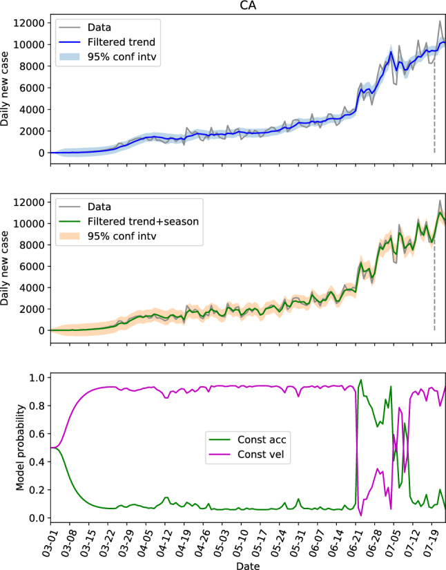
The hidden state estimation of California with trained parameters learned from its own data

Fig. 5.

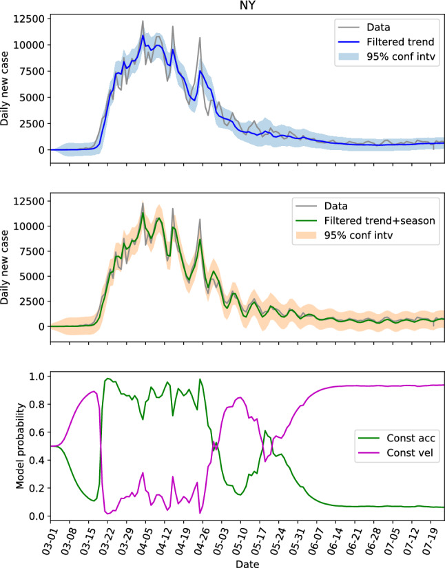
The hidden state estimation of New York with trained parameters learned from its own data

Fig. 6.

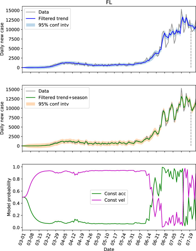
The hidden state estimation of Florida with trained parameters learned from California data

Fig. 7.

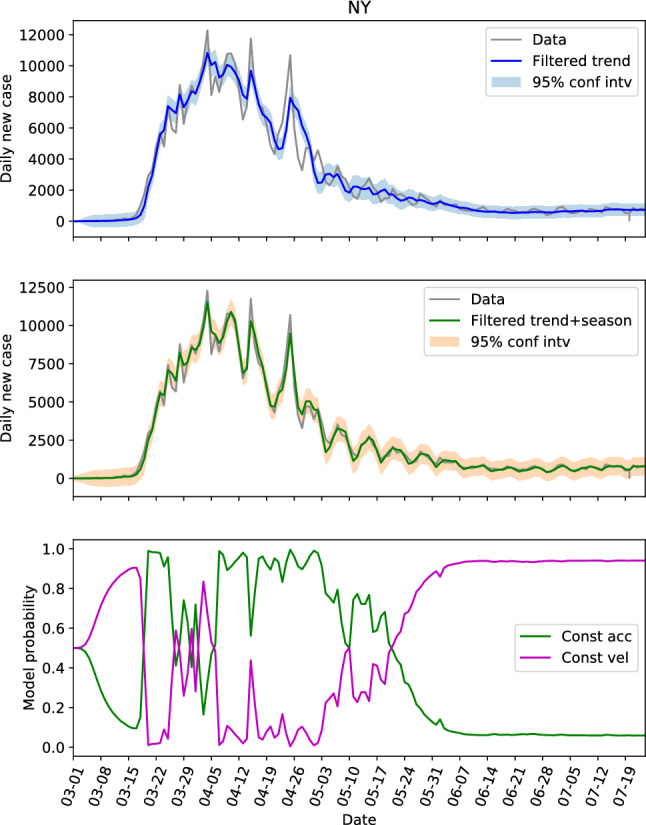
The hidden state estimation of New York with trained parameters learned from California data

Comparing Fig. 4 with Fig. 5, the model probabilities of CA and NY are very different. And the evolutions of the daily new cases of these two states are different too. However, the estimation of the hidden states of NY based on the learned parameter from CA in Fig. 7 resembles Fig. 5 a lot, and the 95% interval of the filtered trend and seasonal components can include the test data well. This not only shows that the hidden states of NY can be estimated via CA data, but also indicates that the model probability is an outcome of combined effects of the learned parameter and the test data (the model probabilities of Figs. 4 and 7 are very different with exactly the same dynamics). For FL, the estimations based on the learned parameters of its own data (Fig. 3b) and the estimations based on the learned parameters of CA data (Fig. 6) are also close.

The hidden state estimations of the three locations with low populations and population densities are shown in Figs. 8, 9 and 10. For NC in Fig. 8, the constant velocity model is superior most of the time, though the advantage is not huge, which is consistent with the steadily increasing of daily new cases. The evolution patterns of the model probability for GA and AL are similar, they both saw the dominance of constant velocity model before June 20 (or near this date), and a switching to more aggressive constant acceleration model after that. Fig. 11 presents the estimations of hidden state for NC again, but with the parameters learned from GA data. Comparing Fig. 11 with Fig. 8, the trend and seasonal behaviors are well captured, the model probability has same pattern of evolution, and the switches between models are also represented. Figure 11 is an example showing that the dynamics are similar within the second group.

Fig. 8.

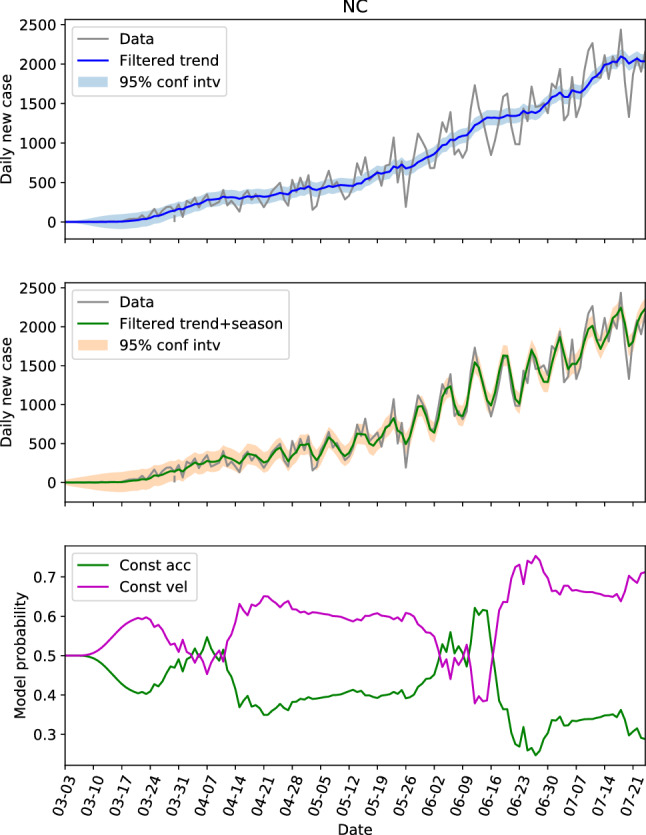
The hidden state estimation of North Carolina with trained parameters learned from its own data

Fig. 9.

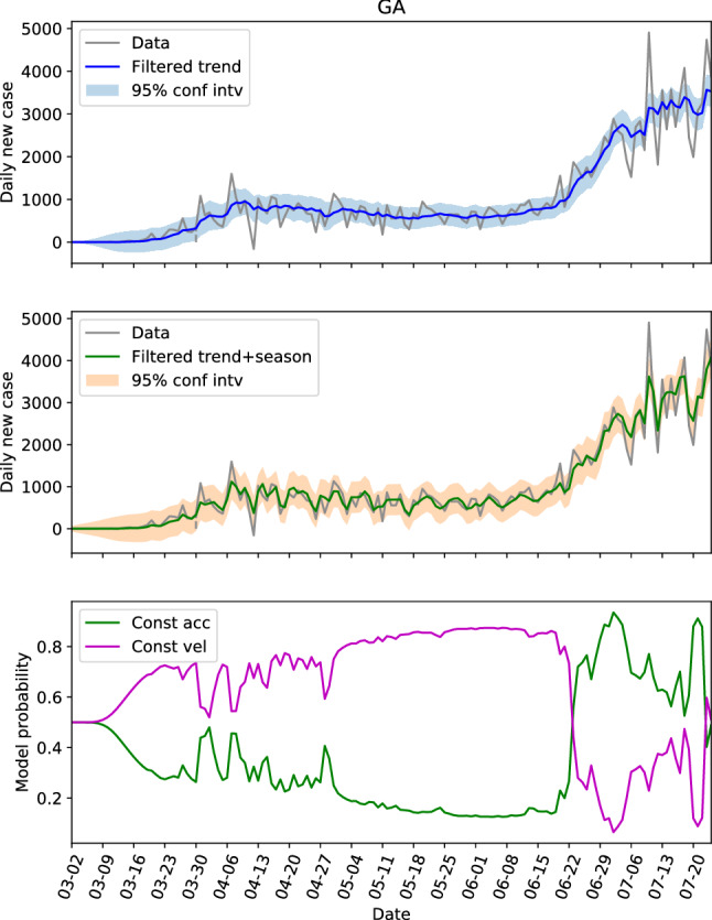
The hidden state estimation of Georgia with trained parameters learned from its own data

Fig. 10.

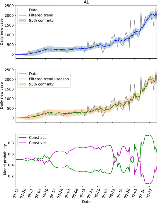
The hidden state estimation of Alabama with trained parameters learned from its own data

Fig. 11.

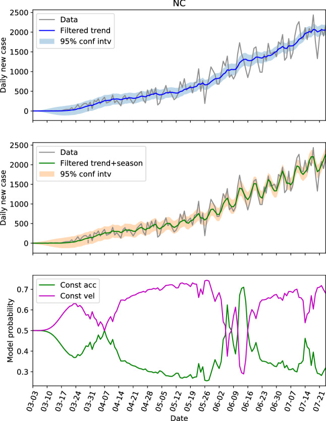
The hidden state estimation of North Carolina with trained parameters learned from Georgia data

Actually, the primary route of transmission of the COVID-19 is by close contact from person-to-person [36], and this makes the population density a vital factor for the spread of the disease. With same dynamics within the first and second groups, respectively, our research indicates that the population density might be the driving force of the spread COVID-19.

The role of model probability

From the previous analysis, we already know that the model probability gives the dominance of the constant acceleration model and constant velocity model, which are associated with quadratic growth and linear growth of the data, respectively.

Another important feature is that the switching from linear growth to quadratic growth usually indicates the change of growth rate. When the data is increasing both before and after the switching, it is a warning sign that the new cases could increase rapidly. Take the US as an example (see in Fig. 2b), the switching at around March 20 from linear growth to quadratic growth warned the rapid increasing of new cases, and the later evolution has confirmed it. The switching at around June 20, also gave a clear sign of increased growth rate, and we saw another rapid increasing of new cases. By the estimations of FL in Fig. 3b and CA in Fig. 4, GA in Fig. 9, Alabama in Fig. 10, and some other locations that are not shown here, for instance TX and AZ, we can see the switches from linear growth to quadratic growth for all these locations at around June 20. The non-accidental similarity gave strong sign of rapid increasing of infections, which could be useful for the decision-making.

On the contrary, the switching from the quadratic growth to linear growth usually gives good sign of either switching to a less aggressive increasing or a stable decreasing stage. Figure 2b of the US data experienced this type of switching at around the end of April, and the data switched to a steady decreasing stage after that. In addition, there is a sign of the switching at July 24, which means the data will hopefully switch from rapid increasing to a less aggressive stage. For CA in Fig. 4, the switching at around July 5 gave a short period of break from a rapid increasing to a less aggressive growth, and it remained at the linear growth stage which indicates that CA could experience a steady growth stage with low rate. One can do the same analysis for other locations.

From the above analysis we see that the model probability plays an important role in exposing the hidden dynamics and making general and non-quantitative predictions. The switching from one model to another gives useful information for the overall trend.

Forecasting

Algorithm 2 described in Sect. 3.3 is used for forecasting of the COVID-19 data. Figures 12 and 13 present the 20 days forecasts of the US and CA at different times, respectively. Of which, the top sub-figures, the second sub-figures from the top, the third sub-figures from the top, and the bottom sub-figures show that forecasts starting from June 28, July 8, July 17 and July 24, respectively. The model probabilities along the forecasts are also presented. The top two sub-figures, where the data of the predicted dates are available, show that the forecasts can capture the future trend well. The predictions with seasonal components are able to recover the cyclic behaviors in the data to some extent. Moreover, the 95% confidence interval of the forecasting is able to include the measurement data but the width of the interval grows very quickly with increased prediction steps. Which means the forecasts by the SKF are more confident in short to middle terms.

Fig. 12.

Daily new cases forecasting of the US by SKF at different times

Fig. 13.

Daily new cases forecasting of California by SKF at different times

For the US in Fig. 12, the trend showed relatively rapid increasing within the 20 days of forecasting starting from June 28. The growth rate was decreased for the forecasts staring from July 8, and the forecasting even switched to decreasing for the forecasts starting from July 17. The model probability of constant acceleration in this case experienced a drop from over 0.8 to approximately 0.6, which resembles a switching from quadratic growth stage to linear growth stage, that is, the rapid growth was tempered. However, this trend was not maintained since the constant acceleration regained its dominance afterward, see in the bottom sub-figure that shows the forecasts starting from July 24. It suggests that the new infections stopped decreasing on July 24 and will be in a flat curve stage.

For CA in Fig. 13, the forecasting starting from June 28 indicated a rapid increasing within 20 days, though the model probability suggested a potential switch from quadratic growth to linear growth. But, if comparing with the trend several steps behind, where the daily new cases just experienced a nearly exponential growth, the increasing rate of the forecasts is still tempered, which is consistent with the change in model probability. The growth rate reduced a lot for the forecasting staring from July 8. The model probability at around July 8 suggested a switching from quadratic growth stage to linear growth stage, and it stayed at the latter. This indicates that the daily case of California is more likely to remain at a linear growth stage after July 8, with a growth rate that is approximately the slope of the trend component. This is verified by the forecasts starting from July 17 and July 24. Both of which gave linear growth forecasts.

For both the US and CA, we can see that the forecasting changes with time progresses. The limitations of the forecasting lie in the observation that prediction could give deviated trend when there is a switch from one model to another. For example in the third sub-figure of Fig. 12, the predicted trend indicated a decrease in new cases, and the dominance of constant acceleration model dropped to the same level of the constant velocity model. However, the constant acceleration model regained its dominance afterwards and the predicted trend in the last sub-figure of Fig. 12 is flattened. In addition, though the forecasts at a stable dynamics (no switch between models) can predict the future trend well, it is not necessarily that the prediction with seasonal components can always capture the cyclic behaviors well. For instance the first sub-figure of Fig. 13, in which the trend of the data is well predicted but the cyclic behavior is not represented well in the predictions of the first several days.

The more quantitative forecasting of this section and the non-quantitative overall prediction by the model probability can be combined for mutual verification and providing more reliable forecasts.

Concluding remarks

In this paper, the SKF with seasonal component is introduced and applied for the dynamics learning and forecasting of the daily new cases of COVID-19 of the US. The optimal parameters of SKF learned from the data is able to capture both the trend and seasonal component, in a sense that the 95% confidence interval is able to include the data with narrow width. The resembles of dynamics at neighborhood period of time is also embedded in the SKF parameters, hence the dynamics learned from previous data is sufficient to estimate the hidden states of future time steps. It is also discovered that the locations with same level of population and population density have similar dynamics, the dynamics of one location can accurately estimate of the hidden state of another. The model probabilities give implications of how the new cases could evolve as well as how the growth rate could change. The switching between models indicated the change of dynamics, hence, in turn, provides useful information for inference and prediction of the overall trend. The multi-step-ahead predictor of SKF provides quantitative forecasts of new cases for both trend and seasonal components. The forecasting will update with the progressing of time and has narrow 95% confidence intervals for short to middle term predictions. The quantitative forecasting can be combined the overall prediction given by the model probabilities to offer more insight on the future trend.

We remark that the effects of social interventions on the pandemic are embedded in the dynamics of the daily new cases data. The changes of public policies can be presented in the switches of the dynamics given by the SKF. The consequences of new major policies can, hence, be observed and predicted by the SKF. The state space matrices $\mathit{A}$, $\mathit{H}$, $\mathit{Q}$ and $\mathit{R}$ are assumed to be constant in the present paper, however, there are changes of dynamics along the time. For instance, the variations of the daily new cases data after June 20, especially for some states like CA, FL, GA and others that are not presented, were obviously larger than the data before. Using an online algorithm to learn the time-varying parameters could improve the SKF method. Moreover, one could also incorporate the SKF method with the SIR family models. Different from the SKF method, where the epidemic features are assumed to be implicitly embedded in the learned dynamics, the SIR family methods describe the dynamics of COVID-19 by epidemic parameters explicitly, for instance the infection rate, recover rate and others. However, different social scenarios are supposed to have different parameters, for instance, the infection rates with and without lock down policies are different, and the infection and recover rates for young and elderly people are different. Different models can be generated with different parameters, and these models can be incorporated into the scheme of SKF. The model probabilities of these models can provide rich information of the effectiveness of social interventions as aforementioned. Linearization techniques of the SIR family model would be required for the incorporation.

References

- 1.Kermack WO, McKendrick AG. Predictive mathematical models of the covid-19 pandemic: underlying principles and value of projections. Ser A Contain Pap Math Phys Character. 1927;115(772):700–721. [Google Scholar]
- 2.Toda AA (2020) Susceptible-infected-recovered (sir) dynamics of covid-19 and economic impact. arXiv:2003.11221
- 3.Fanelli D, Piazza F. Analysis and forecast of covid-19 spreading in China, Italy and France. Chaos Solitons Fractals. 2020;134:109761. doi: 10.1016/j.chaos.2020.109761. [DOI] [PMC free article] [PubMed] [Google Scholar]
- 4.Sarkar K, Khajanchi S, Nieto JJ (2020) Modeling and forecasting the covid-19 pandemic in India. Chaos Solitons Fractals, 110049 [DOI] [PMC free article] [PubMed]
- 5.He S, Peng Y, Sun K (2020) Seir modeling of the covid-19 and its dynamics. Nonlinear Dyn, pp 1–14 [DOI] [PMC free article] [PubMed]
- 6.Linka K, Peirlinck M, Kuhl E (2020) The reproduction number of covid-19 and its correlation with public health interventions. medRxiv [DOI] [PMC free article] [PubMed]
- 7.Roosa K, Lee Y, Luo R, Kirpich A, Rothenberg R, Hyman J, Yan P, Chowell G. Real-time forecasts of the covid-19 epidemic in China from february 5th to february 24th, 2020. Infect Disease Model. 2020;5:256–263. doi: 10.1016/j.idm.2020.02.002. [DOI] [PMC free article] [PubMed] [Google Scholar]
- 8.Petris G, Petrone S, Campagnoli P (2009) Dynamic linear models. In: Dynamic linear models with R. Use R. Springer, New York, NY. 10.1007/b135794_2
- 9.Chakraborty T, Ghosh I (2020) Real-time forecasts and risk assessment of novel coronavirus (covid-19) cases: a data-driven analysis. Chaos Solitons Fractals, 109850 [DOI] [PMC free article] [PubMed]
- 10.Hu Z, Ge Q, Jin L, Xiong M (2020) Artificial intelligence forecasting of covid-19 in China. arXiv:2002.07112 [DOI] [PMC free article] [PubMed]
- 11.Harvey A, Kattuman P (2020) Time series models based on growth curves with applications to forecasting coronavirus. Covid Econ Vetted Real-Time Pap (24)
- 12.Gupta S, Raghuwanshi GS, Chanda A (2020) Effect of weather on COVID-19 spread in the US: a prediction model for India in 2020. Sci Total Environ. 10.1016/j.scitotenv.2020.138860 [DOI] [PMC free article] [PubMed]
- 13.Jewell NP, Lewnard JA, Jewell BL (2020) Predictive mathematical models of the COVID-19 pandemic: underlying principles and value of projections. JAMA 323(19):1893–1894. 10.1001/jama.2020.6585; https://jamanetwork.com/journals/jama/fullarticle/2764824 [DOI] [PubMed]
- 14.Murphy KP (1998) Switching kalman filters. Tech. rep
- 15.Harvey AC (1990) Forecasting, structural time series models and the Kalman filter. Cambridge University Press. https://ideas.repec.org/b/cup/cbooks/9780521321969.html
- 16.Wales DJ, Doye JP. Global optimization by basin-hopping and the lowest energy structures of lennard-jones clusters containing up to 110 atoms. J Phys Chem A. 1997;101(28):5111–5116. doi: 10.1021/jp970984n. [DOI] [Google Scholar]
- 17.Manfredi V, Mahadevan S, Kurose J (2005) Switching kalman filters for prediction and tracking in an adaptive meteorological sensing network. In: 2005 second annual IEEE communications society conference on sensor and Ad Hoc communications and networks, 2005. IEEE SECON 2005. pp 197–206. Citeseer
- 18.Lim P, Goh CK, Tan KC, Dutta P. Multimodal degradation prognostics based on switching kalman filter ensemble. IEEE Trans Neural Netw Learn Syst. 2015;28(1):136–148. doi: 10.1109/TNNLS.2015.2504389. [DOI] [PubMed] [Google Scholar]
- 19.Nguyen LH, Goulet JA. Anomaly detection with the switching kalman filter for structural health monitoring. Struct Control Health Monit. 2018;25(4):e2136. doi: 10.1002/stc.2136. [DOI] [Google Scholar]
- 20.Reuben LCK, Mba D. Diagnostics and prognostics using switching kalman filters. Struct Health Monit. 2014;13(3):296–306. doi: 10.1177/1475921714522844. [DOI] [Google Scholar]
- 21.Cui L, Wang X, Xu Y, Jiang H, Zhou J. A novel switching unscented kalman filter method for remaining useful life prediction of rolling bearing. Measurement. 2019;135:678–684. doi: 10.1016/j.measurement.2018.12.028. [DOI] [Google Scholar]
- 22.Coronavirus (covid-19) data in the united states. https://github.com/nytimes/covid-19-data. Accessed 25 July 2020
- 23.Welch G, Bishop G, et al. (1995) An introduction to the kalman filter
- 24.Musoff H, Zarchan P (2009) Fundamentals of Kalman filtering: a practical approach. American Institute of Aeronautics and Astronautics
- 25.Li X, Wang K, Wang W, Li Y (2010) A multiple object tracking method using kalman filter. In: The 2010 IEEE international conference on information and automation, pp 1862–1866. IEEE
- 26.Cooper S, Durrant-Whyte H (1994) A Kalman filter model for GPS navigation of land vehicles. In Proceedings of IEEE/RSJ international conference on intelligent robots and systems (IROS’94), vol 1. IEEE, pp 157–163. 10.1109/IROS.1994.407396. https://ieeexplore.ieee.org/document/407396
- 27.Lopes HF, Tsay RS. Particle filters and bayesian inference in financial econometrics. J Forecast. 2011;30(1):168–209. doi: 10.1002/for.1195. [DOI] [Google Scholar]
- 28.Wu W, Black MJ, Mumford D, Gao Y, Bienenstock E, Donoghue JP. Modeling and decoding motor cortical activity using a switching kalman filter. IEEE Trans Biomed Eng. 2004;51(6):933–942. doi: 10.1109/TBME.2004.826666. [DOI] [PubMed] [Google Scholar]
- 29.Casella G, Berger RL. Statistical inference. Pacific Grove: Duxbury Pacific Grove; 2002. [Google Scholar]
- 30.Brockwell PJ, Davis RA, Fienberg SE. Time series: theory and methods: theory and methods. Berlin: Springer; 1991. [Google Scholar]
- 31.West M, Harrison J (2006) Bayesian forecasting and dynamic models. Springer. 10.1007/978-1-4757-9365-9
- 32.Jalles JT (2009) Structural time series models and the kalman filter: a concise review
- 33.Interim clinical guidance for management of patients with confirmed coronavirus disease (covid-19). https://www.cdc.gov/coronavirus/2019-ncov/hcp/clinical-guidance-management-patients.html. Accessed 25 July 2020
- 34.What you need to know about covid-19. https://covid19.lacounty.gov/testing-faq/. Accessed 25 July 2020
- 35.Akhlaghi S, Zhou N, Huang Z (2017) Adaptive adjustment of noise covariance in kalman filter for dynamic state estimation. In: 2017 IEEE power & energy society general meeting, pp. 1–5. IEEE
- 36.Cdc updates covid-19 transmission webpage to clarify information about types of spread. https://www.cdc.gov/media/releases/2020/s0522-cdc-updates-covid-transmission.html. Accessed 25 July 2020