COVID-19 Pandemic: ARIMA and Regression Model-Based Worldwide Death Cases Predictions

Abstract

COVID-19 has now taken a frightening form. As the days pass, it is becoming more and more widespread and now it has become an epidemic. The death rate, which was earlier in the hundreds, changed to thousands and then progressed to millions. If the same situation persists over time, the day is not far when the humanity of all the countries on the globe will be endangered and we yearn for breath. From January 2020 till now, many scientists, researchers and doctors have been trying to solve this complex problem so that proper arrangements can be made by the governments in the hospitals and the death rate can be reduced. The presented research article shows the estimated mortality rate by the ARIMA model and the regression model. This dataset has been collected precisely from DataHub-Novel Coronavirus 2019-Dataset from 22nd January to 29th June 2020. To show the current mortality rate of the entire subject, the correlation coefficients of attributes (MAE, MSE, RMSE and MAPE) were used, where the average absolute percentage error validated the model by 99.09%. The ARIMA model is used to generate auto_arima SARIMAX results, auto_arima residual plots, ARIMA model results, and corresponding prediction plots on the training dataset. These data indicate a continuous decline in death cases. By applying a regression model, the coefficients generated by the regression model are estimated, and the actual death cases and expected death cases are compared and analyzed. It is found that the predicted mortality rate has decreased after May 2, 2020. It will help the government and doctors prepare for the forthcoming plans. Based on short-period predictions, these methods can be used to forecast the mortality rate for a long period.

Introduction

As indicated by the World Health Organization, the COVID-19 virus is a communicable disease that spreads from one person to another. Personal contact and small droplets in the breath of infected person can cause the virus to spread to others and cause severe acute respiratory syndrome [1]. In 2020 of January, WHO initially informed the humanity regarding pneumonia for obscure reasons, and the world came to know that this disease spread from person to person [2]. The incidence of this mysterious disease started from a city called Wuhan of China [3]. The status report of WHO says that till date from January 15, 2020 to July 1, 2020; 507,435 people have lost their lives worldwide and this number is continuously increasing [4]. The group of RNA viruses are called coronavirus [5]. In humans, it causes respiratory tract infections. It has SARS, MERS and COVID-19 deadly varieties. There are no immunizations or antiviral medications to protect from corona infection in people yet. Common symptoms include high fever, tiredness, cough, shortness of breath, and loss of taste and smell, and complications include pneumonia and acute breathing infection [6]. The confirmation of the first death case from Asia to Europe was as follows: initial confirmed casualty in Wuhan, China on 9th of January, 2020, initial confirmed death in Philippines outside China on February 1, 2020, and on February 14, 2020 the first confirmed death in the European country France [7]. The ratio of death rate is 5.4% till 16 June 2020 against 437,283 deaths for 8051,732 cases. This number may vary from time to time and region to region [8].

The motto of our research is to predict the future of death cases based on machine learning regression model as well as time series ARIMA model. Both models are used to predict the future values. No eye-catching and extensively tested antibody against COVID-19 has been designed; more importantly, the key part of the subsequent response to this pandemic is to reduce the spread of the pandemic, or to smooth the curve. The work of information researchers and information mining analysts is to coordinate relevant information and it is more likely to help to understand the infection and its quality, which helps to make the right choices and solid activities. This will prompt people to take stronger measures to establish frameworks, medicine, antibodies and control of comparable pandemics with greater prospects. The aims of the present investigation are as follows.

1. Displaying the current mortality rate and corresponding measures, as shown on the graph.

2. Extracting different statistical measures from these graphs.

3. Using ARIMA and regression models to predict and find future deaths worldwide.

Except for the first part of the introduction, the structure of the remaining research papers is as follows:

Section II: background, Section III: methodology, Section IV: dataset description and analysis, Section V: results and discussion, Section VI: conclusion.

Background

Although it has been about 6 months since the COVID-19 pandemic has spread, many researchers have done a lot of work on it and it is being worked on continuously. The following is a description of some of the researches presented.

Benvenuto et al. [9] carried out an ARIMA model forecast on COVID-2019 using information gathered from Johns Hopkins epidemiological department of the predominance and rate. For additional correlation or from a future point of view, case definitions and information assortment must be kept up progressively.

Comprehensive information related to COVID-19 was collected from WHO website from February 21 to April 15, 2020 by Zeynep Ceylan [10]. Some ARIMA models with different ARIMA boundaries were selected, which includes ARIMA (0, 2, 1) for the lowest MAPE (4.7520) for Italy similarly for Spain and France selected separately with ARIMA (1, 2, 0) and ARIMA (0, 2, 1) and the lowest MAPE (5.58486) and (5.6335), respectively. This test shows that the ARIMA model is appropriate to understand the effect of COVID-19. The aftereffects of the examination can reveal insight into understanding the patterns of the episode and give a thought of the epidemiological phase of these locales.

In Mhdm et al. [11], for the purpose of time series analysis, different models such as ARIMA, CUBIST, RF, RIDGE, SVR and stacking-ensemble method were assessed. The created models can produce exact forecasting, with errors of 0.87–3.51%, 1.02–5.63%, and 0.95–6.90% in 1, 3, and 6 days, respectively. The positioning of models, from the best to the most noticeably worst with respect to precision, in all situations is SVR, stacking–gathering learning, ARIMA, CUBIST, RIDGE, and RF models.

In Pandey et al. [12], in this inspection, until March 30, 2020, this scene of suffering in India was meticulous, and the number of cases in the next 14 days was evaluated. Taking into account the data accumulated from the Johns Hopkins University depository in the period from January 30, 2020 to March 30, 2020, the SEIR model and the regression model were used. RMSLE evaluated the introduction of the model, and the data of the SEIR model were 1.52 and 1.75, respectively. The RMSLE tightening rate between the SEIR model and the regression model is 2.01. In addition, the estimation of R 0 as the diffusion of pollution was analyzed to 2.02. It is foreseeable that in the next 14 days, the number of cases may rise to 5000–6000.

Chakraborty and Ghosh [13] collected the data as of April 4, 2020, and showed a pandemic flare-up in excess of 1116,643 affirmed diseases and in excess of 59,170 revealed deaths around the world. The primary objective of this paper is twofold (1) producing present moment (constant) estimates of things to come COVID-19 cases for various nations; (2) chance evaluation of the novel COVID-19 for some significantly influenced nations. To take care of the primary issue, they introduced a half breed approach dependent on ARIMA model and wavelet-based forecasting model that can create present moment (10 days ahead) conjectures of the quantity of day by day affirmed cases for Canada, France, India, South Korea, and the UK. They applied an ideal relapse tree calculation to discover basic causal factors that altogether influence the case casualty rates for various nations.

Chintalapudi et al. [14] studied, from mid-February to the end of March, COVID-19 data of deleted cases registered and restored on-site by the Italian Ministry of Health. Appointment of the accidental ARIMA vision group using R real model was completed. The accuracy of the enrollment case model reached 93.75%, and the accuracy of the recovery case model reached 84.4%. At the end of May, the forecasting of infected patients could be reach the value of 182,757, and recovered cases could be registered value of 81,635. Their findings indicate that it is possible to reduce enrollment of cases by approximately 35% and improve recovery of cases by approximately 66%.

According to Vardavas and Nikitara [15] from March 18, 2020, there were a total of 194,909 COVID-19 patients, including 7876 deaths, a large part of which were in China (3242) and Italy (2505). In their multivariate key back slip test, chronic diseases and smoking are risk factors for disease development (OR = 14.28; 95% CI 1.58–25.00; p = 0.018). From the data they calculate that the smokers were 1.4 times more likely (RR = 1.4, 95% CI 0.98–2.00) to have severe symptoms of COVID-19 and approximately 2.4 times more likely to be admitted to an ICU, requiring mechanical ventilation or passage, which is different from non-smokers (RR = 2.4, 95% CI 1.43–4.04).

Yan et al. [16] calculated the relapse rate used to sense signs associated with COVID-19 positivity. Between March 3, 2020 and March 29, 2020, a total of 1480 patients with influenza-like reactions underwent the COVID-19 test. Our assessment yielded 59 out of 102 (58%) COVID-19-positive patients and 203 out of 1378 COVID-19-negative patients (15%). Of COVID-19-positive subjects, 68% (40/59) and 71% (42/59) had loss of odor and taste symptoms, respectively, and 16% (33/203) and 17% (35/203) of subjects has different symptoms as compared to COVID-19 negative patients (p < 0.001). In addition, odor impairment and COVID-19 positivity (anosmia: adjusted odds ratio [aOR] 10.9; 95% CI 5.08–23.5; ageusia: aOR 10.2; 95% CI 4.74–22.1), but the sore throat is related to the COVID-19 enemy (aOR 0.23; 95% CI 0.11–0.50). Of the patients who reported loss of olfaction associated with COVID-19, 74% (28/38) of the patients also had insomnia.

Methodology

In this section, we collected data from DataHub-Novel Coronavirus 2019-Dataset. The dataset includes information on patients with COVID-19 dated from January 22, 2020 to June 20, 2020. The dataset has the attributes of globally confirmed cases, rehabilitation cases, death cases and COVID-19 prevalence. There are basically two methods for analyzing the outbreak of a pandemic. Both ARIMA and regression models are used to predict future value. In this sense, we have basically analyzed the correlation between mortality and all precious attributes.

ARIMA Model

Since the administrator needs to carefully consider the time of sick leave, this exploratory paper proposes an inspection of the autoregressive merged moving normal model. The ARIMA model is additionally utilized as a proficient device to design assets, for example, pandemic and groups for the crisis department [17, 18]. Another relevance of the ARIMA model is to foresee and contemplate the impact of COVID-19 [19–21].

Time series forecasting-based specific sort of forecasting strategy is called ARIMA modeling. ARIMA or “Auto Regressive Integrated Moving Average” is really a class of models that clarifies a given time arrangement dependent on its own past qualities, that is, its own limitations and the forecast errors, with the goal that condition can be utilized to figure future values. Mathematically, non-seasonal ARIMA model is define as follows:

An ARIMA model is portrayed by three terms—p, d, q,

where p is the order for the autoregressive expression, q is the order for the moving average expression, d is the number of difference required for making the time arrangement fixed.

The estimation of d is the base number of difference expected to make the difference fixed. What is more, on the off chance that the time difference is now fixed, at that point d = 0.

p is the request for the AR term. It alludes to the quantity of instances of Y to be utilized as indicators. Furthermore, q is the request for the MA term. It alludes to the quantity of dull forecast errors that ought to go into the ARIMA model.

An unadulterated AR model is one where Y_t relies just upon its own instances. That is, Y_t is an element of the ‘instances of Y_t’.

$$Y_t=\alpha +{\beta }_1{Y}_{t-1}+{\beta }_2{Y}_{t-2}+\cdots +{\beta }_p{Y}_{t-p}+{ϵ}_1,$$

where Y_t–1 is the lag1 of the arrangement, β₁ is the coefficient of lag1 that the model evaluates and α is the block term, additionally assessed by the model.

Moreover, an unadulterated MA model is one where Y_t relies just upon the dull forecast errors.

$$Y_t=\alpha +{ϵ}_t+{\varphi }_1{ϵ}_{t-1}+{\varphi }_2{ϵ}_{t-2}+\cdots +{\varphi }_q{ϵ}_{t-q},$$

where the error terms are the errors of the autoregressive model of the particular instances. The mistakes ϵ_t and ϵ_t–1 are the errors from the accompanying conditions:

$$Y_t={\beta }_1{Y}_{t-1}+{\beta }_2{Y}_{t-2}+\cdots +{\beta }_0{Y}_0+{ϵ}_t\text{AR model},$$

$$Y_{t-1}={\beta }_1{Y}_{t-2}+{\beta }_2{Y}_{t-3}+\cdots +{\beta }_0{Y}_0+{ϵ}_{t-1}\text{MA model}.$$

An ARIMA model is one where the time series was differenced at least once to make it stationary and we combine the AR and the MA expressions. So the condition becomes

$$Y_t=\alpha +{\beta }_1{Y}_{t-1}+{\beta }_2{Y}_{t-2}+\cdots +{\beta }_p{Y}_{t-p}{ϵ}_t+{\varphi }_1{ϵ}_{t-1}+{\varphi }_2{ϵ}_{t-2}+\cdots +{\varphi }_q{ϵ}_{t-q}.$$

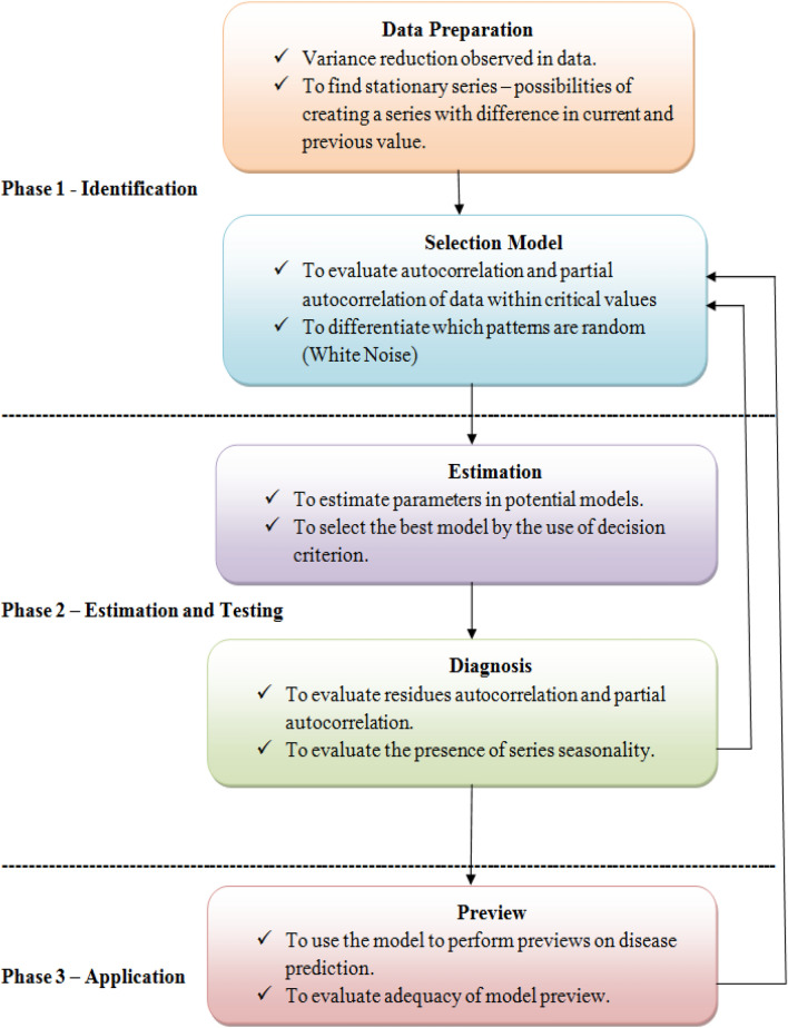
There are many aspects that need attention when making explicit models. With regard to illness, executives need 4 years of information in any situation until the first month of intervention. Subsequently, the model can place examples that might be involved in the arrangement of parameters [22]. Figure 1 below depicts the system implementation of the ARIMA model in disease prediction.

Fig. 1.

A schematic diagram of the ARIMA strategy estimation model. The general association of non-incidental models is ARIMA (p, d, q) [27]

Regression Model

Linear regression is a prescient measurable methodology for displaying connection between a dependent variable with a given arrangement of autonomous factors. It is a direct way to deal with displaying the connection between a dependent variable and at least one independent variable. At the point when we have just a single independent variable, it is as called straightforward linear regression. For more than one independent factor, the procedure is called multiple linear regressions. This investigation has utilized linear regression and multiple regressions for expectation of COVID-19 cases [12].

The linear regression description includes a linear condition that adds a specific information literacy particular arrangement x, whose response is the predictable return y of the data particular arrangement (y). The linear condition gives each information value or part a scale factor, called the coefficient, which is represented by the Greek word beta β. Including an additional coefficient in the same way provides additional degrees of freedom for the line and is repeatedly called the intercept or offset coefficient.

In a straightforward regression issue, the type of the model would be:

$$y={\beta }_0+{\beta }_{1}x,$$

where β₀ is the intercept, β₁ is the coefficient, x is the independent variable, and y is the dependent variable.

In higher estimates, when we have multiple information x, the line is called a plane or hyperplane. Described in this way are the kinds of conditions and specific characteristics for the coefficients (β₀ and β₁).

The general condition for a multiple linear regression with n independent factors is:

$$y={\beta }_0+{\beta }_1{x}_1+{\beta }_1{x}_2+\cdots +{\beta }_n{x}_n+\epsilon ,$$

where β_0, β_1, β_2… β_n are the coefficients, x_1, x_{2, ….} x_n–x are the variables, y is the y-variable, and ϵ is the random error “noise”.

Dataset Description and Analysis

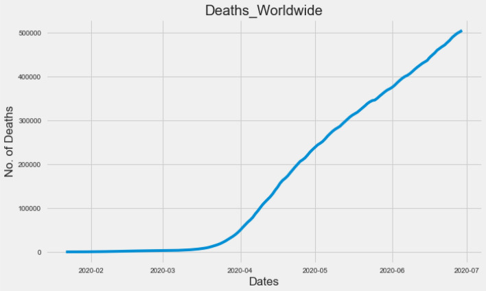
The COVID-19 dataset is taken from the DataHub-Novel Coronavirus dataset from January 22, 2020 to June 29, 2020. It contains five independent attributes, such as date, confirmed cases, rehabilitation cases, death and growth rate, and 160 instances. As we have seen in the dataset, the death toll has increased over time until June 29. This is confirmed by Fig. 2.

Fig. 2.

Confirmed death cases worldwide increasing continuously

Results and Discussion

The earliest COVID-19 patients were recorded in the dataset on January 22, 2020. We have taken examples from January 22, 2020 to June 29, 2020. It consists of 160 instances and five attributes. These attributes have information about the date of recording, confirmed cases, recovered cases, deaths, and growth rates related to COVID-19 patients. The following estimates are made from the dataset to explore and extract useful information.

Correlation Coefficients

The statistical measure correlation coefficient is the strength of the relationship between the relative motions of two variables. The range is defined as − 1 to + 1. Incorrect correlation measurement occurs when the values are greater than + 1 and less than − 1. The correlation measurement at − 1 is completely negative, the correlation measurement at + 1 is positive, and the value at 0.0 is the nonlinear relationship between the two variables [23].

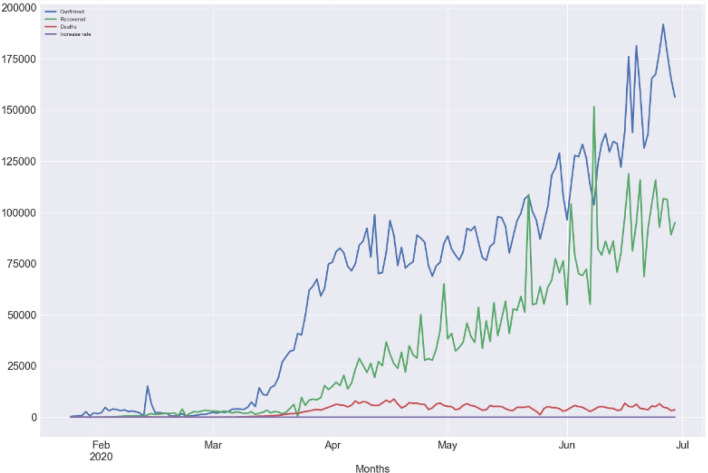
Related statistics can be used to define the relationship between different attributes of the disease. A correlation coefficient can be calculated to determine the correlation level between the confirmed cases and the recovered cases under the current pandemic situation and the rate of increase in deaths and mortality, as shown in Table 1 and Fig. 3. We found that in COVID-19 confirmed case and recovered case, the correlation between these two variables is highly positive.

Table 1.

Correlation coefficients of attributes

	Confirmed	Recovered	Deaths	Increase rate
Confirmed	1.000000	0.986051	0.988177	– 0.378478
Recovered	0.986051	1.000000	0.950569	– 0.337027
Deaths	0.988177	0.950569	1.000000	– 0.401742
Increase rate	– 0.378478	– 0.337027	– 0.401742	1.000000

Fig. 3.

Visual presentation of correlated coefficients

ARIMA Model Results

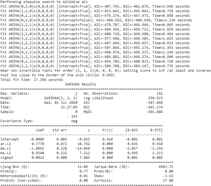
In the ARIMA model, we choose the parameters p, d, q. For this reason, even without drawing graphics, we use auro_arima to find the appropriate parameters. The auro_arima works by directing difference tests like Kwiatkowski–Phillips–Schmidt–Shin, Augmented Dickey-Fuller or Phillips–Perron to decide the request for difference, d, and afterward fitting models inside scopes of characterized start_p, max_p, start_q, max_q ranges [24]. In the event that the occasional discretionary is empowered, auto_arima likewise tries to distinguish the ideal p and q hyperboundaries in the wake of directing the Canova–Hansen to decide the ideal request of occasional difference, d. Figure 4 shows the parameters obtained by the auro_arima model.

Fig. 4.

Auto_arima parameters obtained on train dataset

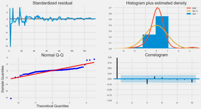
When viewing the residual plot from the auto_arima model, as shown in Fig. 5.

Fig. 5.

Residuals plot by auto_arima

The output of the auto_arema model is explained as follows:

• Standardized residual: The error of the residual is near the mean of the zero line and has a uniform variance.

• Histogram and density plot: In the figure below, the density plot shows the equal distribution around the zero line average.

• QQ-plot: In the QQ chart, all blue dots (ordered distribution of residuals) are on the red line, and any deviations will be skewed by the line. It is usually distributed along N (0, 1) and is considered to be uniformly distributed.

• Correlogram: Correlogram or ACF plots show that the residual error is not autocorrelated. Any autocorrelation implies the residual error.

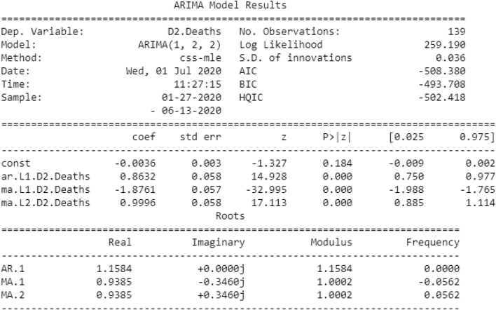
The optimal values of p, d, and q obtained by the auto_arima model are 1, 2, and 2, respectively. Now, using the best parameters obtained (1, 2, 2) to create an ARIMA model, the results are shown in Fig. 6.

Fig. 6.

Results of the ARIMA model

Figure 6 above shows the importance of the ARIMA model. In this figure, we will focus on the coefficient table. The coefficient section shows the weight of each element and how each element affects the time series. p >|z|: this section provides advice on the importance of the weight of each element. Here, the p value of each weight is less than or close to 0.05, so it is wise to include each weight in our model.

These views make us think that our model can create a good fit, which can help us understand time series information and calculate future value. Although we have a reasonable fit, we can occasionally change some limitations of the ARIMA model to improve the model's aggressiveness. We have obtained a model for the time series and can now use it to create estimates [25]. We first compare the predicted value with the actual estimated value of the time series, which will help us understand the accuracy of the prediction. The numbers and associated confidence intervals we have now created can now be used to additionally understand time series and predict what to store. Our data show that relying on time series can maintain a consistent growth rate.

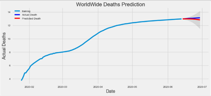
As our predictions for the future say, it is normal to be less optimistic about our values. This is reflected by the deterministic interval generated by our model; as we further develop, the deterministic interval will become larger and larger. We start predicting death cases in a test dataset that maintains 95% confidence. Figure 7 shows the prediction results.

Fig. 7.

Prediction of death cases compared to actual death cases over the training dataset

In the figure, the actual deaths of the training dataset are shown by the blue line, and the predicted deaths are shown by the red line. The prediction of death on the red line has dropped, which means that in the future, the incidence of deaths will become shorter and shorter, as more and more people recover quickly and people maintain the social distance in this pandemic situation.

By using statistical data, we created summary metrics that classify and collect residuals into single value, which are related to the model’s a predictive ability.

To judge the prediction results, let us apply commonly used accuracy indicators; the results are shown in Table 2.

Table 2.

Correlation coefficients of attributes

Measures of accuracy	Value
Mean absolute error (MAE)	0.12044588473307338
Mean squared error (MSE)	0.023012953284359018
Root mean squared error (RMSE)	0.15170020858376898
Mean absolute percentage error (MAPE)	0.009196691386663233

The MAE of our model is 0.1204, which is quite small, and suppose our data death case starts at 0.01.

For MSE, the value 0.0230 is less than MAE. We found this to be the case: MSE is an order of magnitude smaller than MAE.

The value 0.1517 of RMSE is similar to standard deviation and is a measure of how much the residual distribution is.

Around 0.91% MAPE implies the model is about 99.09% accurate in predicting the test set observations.

Regression Model Results

To find out which factor has the most significant influence on the forecasted output and how the various factors identify each other, we will consider different input functions such as “confirmation case”, “recovered case” and “increase rate”. Based on these characteristics, we will predict the deaths of COVID-19 patients. The dataset is split into 80%:20% training and testing, respectively.

In multiple linear regression, the regression model has selected the best coefficients for all attributes [26]. The coefficients of the regression model are shown in Table 3.

Table 3.

Coefficients of regression model

Attributes	Coefficient
Confirmed	0.103305
Recovered	– 0.100568
Increase rate	69.616876

From Table 3, it is clear that if there is increase in “recovered case” by 1 unit, there is a decrease of “death case” by 0.1005 units and vice versa. Similarly, if there is increase in “confirmed case” and “increase rate” by 1 unit, there is increase in “death case” by 0.1033 units and 69.6168 units, respectively.

Now, we predict the test data to check the difference between the actual value and the predicted value in Table 4.

Table 4.

Difference between the actual value and predicted value

Instance number	Actual value	Predicted value
110	286,697	221,975.301362
112	297,539	286,646.565236
143	430,047	423,127.482077
7	133	– 6528.684075
44	3459	– 2713.950271
101	244,129	236,968.993751
122	342,565	329,894.990367
66	31,990	47,224.597929
85	148,157	160,515.287829
86	157,022	167,041.159151
133	386,298	376,198.729391
92	193,926	198,189.689192
26	1868	– 1385.556916
146	443,685	438,945.896459
119	328,483	318,945.015040
62	19,026	25,233.066196
51	5411	808.770349
97	221,109	221,511.564448
128	365,380	355,638.073651
90	180,475	187,102.115303

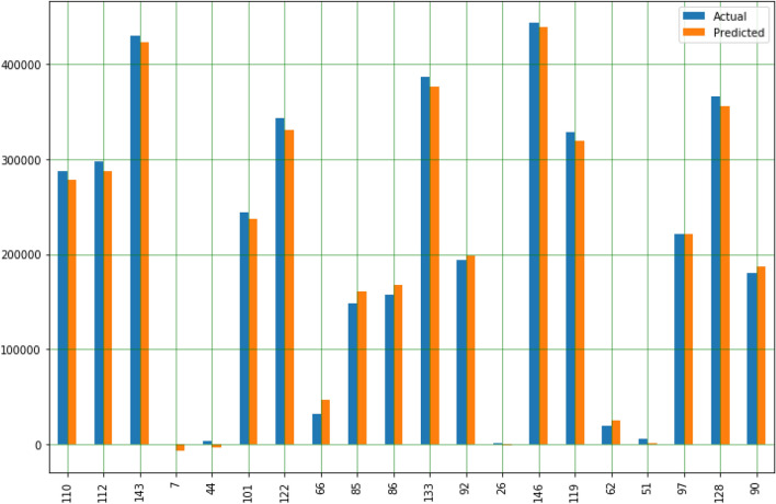
The plot and comparison of the actual value and the predicted value, as shown in Fig. 8.

Fig. 8.

Comparison plot of actual and predicted values of death cases

As shown in the multiple regression model in Table 3 and Fig. 8, the initial predicted number of deaths has increased compared with actual deaths, but as we progress in the data table, compared with actual deaths, the predicted number of deaths decreased from the month of May 2nd 2020.

Overall, this study shows that the reduction in deaths worldwide is a good sign for human society.

Conclusion

In this study, two AI models, ARIMA and regression models, were used to decompose and predict changes in the spread of COVID-19 infection. We have investigated this information and predicted that the number of deaths will be reduced compared to the overall situation. The decline shown in the ARIMA model graph (Fig. 7) indicates that the future mortality rate will decrease (based on the current situation). The training dataset verified by the mean absolute percentage error (MAPE = 99.09%) indicates the accuracy of the model. The regression model also indicated an increase in the initial number of deaths, but over time, it predicted fewer deaths than actual deaths (Table 4; Fig. 8) from 2nd May 2020.

Based on the above results and discussion, through ARIMA and regression models, we can conclude that there is a possibility of reducing deaths worldwide and should be reduced. Over time, there must be new opportunities to deal with this pandemic. Many researchers, scientists, doctors, nurses, medical support staff, and government agencies are all playing their roles. However, we ourselves have a responsibility to follow the guidelines provided by these agencies. If we do not maintain social estrangement, gather in public places, and do not keep the neighborhood clean, how can we overcome the COVID-19 pandemic?

Compliance with Ethical Standards

Conflict of interest

The authors declare that they have no competing interests.

Research involving human participants and/or animals

For this type of study formal consent is not required.

Informed consent

Informed consent was not needed for the study.

References

- 1.World Health Organization. Coronavirus disease 2019 (COVID-19): situation report. 2020. p. 67. https://www.who.int/emergencies/diseases/novelcoronavirus-2019/situation-reports.
- 2.Kessler G. Trump’s false claim that the WHO said the coronavirus was ‘not communicable’. The Washington Post. Archived from the original on April 17, 2020. Retrieved 17 April 2020 from http://archive.is/7Pgq4.
- 3.WHO. Pneumonia of unknown cause—China. WHO. Archived from the original on 7 January 2020. Retrieved 9 April 2020 from https://www.who.int/csr/don/05-january-2020-pneumonia-of-unkown-cause-china/en/.
- 4.Coronavirus disease (COVID-19). Situation Report—147 data as received by WHO from national authorities by 10:00 CEST, 15 June 2020. https://www.who.int/docs/default-source/coronaviruse/situation-reports/20200615-covid-19-sitrep-147.pdf?sfvrsn=2497a605_4.
- 5.Woo PC, Huang Y, Lau SK, Yuen KY. Coronavirus genomics and bioinformatics analysis. Viruses. 2010;2(8):1804–1820. doi: 10.3390/v2081803. [DOI] [PMC free article] [PubMed] [Google Scholar]
- 6.Coronavirus Disease 2019 (COVID-19)—Symptoms. U.S. Centers for Disease Control and Prevention (CDC). 2020. Retrieved 21 March 2020 from https://www.cdc.gov/coronavirus/2019-ncov/symptoms-testing/symptoms.html.
- 7.Coronavirus live updates: first death outside Asia reported in France. The New York Times. 2020. Retrieved 15 February 2020 from https://www.nytimes.com/2020/02/15/world/europe/france-coronarivus-death.html.
- 8.COVID-19 Dashboard by the Center for Systems Science and Engineering (CSSE) at Johns Hopkins University (JHU). ArcGIS. Johns Hopkins University. 2020. https://gisanddata.maps.arcgis.com/apps/opsdashboard/index.html#/bda7594740fd40299423467b48e9ecf6.
- 9.Benvenuto D, Giovanetti M, Vassallo L, Angeletti S, Ciccozzi M. Data in brief application of the ARIMA model on the COVID- 2019 epidemic dataset. Data Br. 2020 doi: 10.1016/j.dib.2020.105340. [DOI] [PMC free article] [PubMed] [Google Scholar]
- 10.Zeynep Ceylan , “Estimation of COVID-19 Prevalence in Italy, Spain, and France”, PMID: 32360907 PMCID: PMC7175852. 2020;10.1016/j.scitotenv.2020.138817. [DOI] [PMC free article] [PubMed]
- 11.Mhdm R, Silva RG, Mariani VC, Coelho LS. Short-term forecasting COVID-19 cumulative confirmed cases: perspectives for Brazil. Chaos Solitons Fractals. 2020 doi: 10.1016/j.chaos.2020.109853. [DOI] [PMC free article] [PubMed] [Google Scholar]
- 12.Pandey G, Chaudhary P, Gupta R, Pal S. SEIR and regression model based COVID-19 outbreak predictions in India. arXiv 2020, arXiv:2004.00958.
- 13.Chakraborty T, Ghosh I. Real-time forecasts and risk assessment of novel coronavirus (COVID-19) cases: a data-driven analysis. Chaos Solitons Fractals. 2020 doi: 10.1016/j.chaos.2020.109850. [DOI] [PMC free article] [PubMed] [Google Scholar]
- 14.Chintalapudi N, Battineni G, Battineni F. COVID-19 virus outbreak forecasting of registered and recovered cases after sixty day lockdown in Italy: a data driven model approach. J Microbiol Immunol Infect. 2020;53:396–403. doi: 10.1016/j.jmii.2020.04.004. [DOI] [PMC free article] [PubMed] [Google Scholar]
- 15.Vardavas CI, Nikitara K. COVID-19 and smoking: a systematic review of the evidence. Tob Induc Dis. 2020;18:20. doi: 10.18332/tid/119324. [DOI] [PMC free article] [PubMed] [Google Scholar]
- 16.Yan CH, Faraji M, Prajapati DP, Boone CE. Association of chemosensory dysfunction and COVID-19 in patients presenting with influenza-like symptoms. Int Forum Allergy Rhinol. (in press). 10.1002/alr.22579. (Epub 12 April 2020) [DOI] [PMC free article] [PubMed]
- 17.Sun Y, Heng B, Seow Y, Seow E. Forecasting daily attendances at an emergency department to aid resource planning. BMC Emerg Med. 2009;9:1–1. doi: 10.1186/1471-227X-9-1. [DOI] [PMC free article] [PubMed] [Google Scholar]
- 18.Rathlev NK, Chessare J, Olshaker J, Obendorfer D, Mehta SD, Rothenhaus T, et al. Time series analysis of variables associated with daily mean emergency department length of stay. Ann Emerg Med. 2007;49(3):265–271. doi: 10.1016/j.annemergmed.2006.11.007. [DOI] [PubMed] [Google Scholar]
- 19.López-Lozano JM, Monnet DL, Yagüe A, Burgos A, Gonzalo N, Campillos P, et al. Modelling and forecasting antimicrobial resistance and its dynamic relationship to antimicrobial use: a time series analysis. Int J Antimicrob Agents. 2000;14(1):21–31. doi: 10.1016/S0924-8579(99)00135-1. [DOI] [PubMed] [Google Scholar]
- 20.Hsueh PR, Chen WH, Luh KT. Relationships between antimicrobial use and antimicrobial resistance in Gram-negative bacteria causing nosocomial infections from 1991–2003 at a university hospital in Taiwan. Int J Antimicrob Agents. 2005;26(6):463–472. doi: 10.1016/j.ijantimicag.2005.08.016. [DOI] [PMC free article] [PubMed] [Google Scholar]
- 21.Aldeyab MA, Monnet DL, López-Lozano JM, Hughes CM, Scott MG, Kearney MP, et al. Modelling the impact of antibiotic use and infection control practices on the incidence of hospital-acquired methicillin-resistant Staphylococcus aureus: a time series analysis. J Antimicrob Chemother. 2008;62(3):593–600. doi: 10.1093/jac/dkn198. [DOI] [PubMed] [Google Scholar]
- 22.Linden A, Adams JL, Roberts N. Evaluating disease management program effectiveness: an introduction to time series analysis. Dis Manag. 2003;6(4):243–255. doi: 10.1089/109350703322682559. [DOI] [PubMed] [Google Scholar]
- 23.Meng X, Rosenthal R, Rubin DB. Comparing correlated correlation coefficients. Psychol Bull. 1992;111:172–175. doi: 10.1037/0033-2909.111.1.172. [DOI] [Google Scholar]
- 24.Manoj K, Madhu A. An application of time series arima forecasting model for predicting sugarcane production in India[J] Stud ITI Bus Econ. 2014;9(1):81–94. [Google Scholar]
- 25.Calheiros RN, Masoumi E, Ranjan R, Buyya R. Workload prediction using ARIMA model and its impact on cloud applications’ QoS. IEEE Trans Cloud Comput. 2015;3:4. doi: 10.1109/TCC.2014.2350475. [DOI] [Google Scholar]
- 26.Catalina T, Iordache V, Caracaleanu B. Multiple regression model for fast prediction of the heating energy demand. Energy Build. 2013;57(302–12):28. [Google Scholar]
- 27.Sato RC. Disease management with ARIMA model in time series. Einstein. 2013;11(1):128–131. doi: 10.1590/S1679-45082013000100024. [DOI] [PMC free article] [PubMed] [Google Scholar]