

Abstract
TROPOMI satellite data show substantial drops in nitrogen dioxide (NO2) during COVID‐19 physical distancing. To attribute NO2 changes to NO x emissions changes over short timescales, one must account for meteorology. We find that meteorological patterns were especially favorable for low NO2 in much of the United States in spring 2020, complicating comparisons with spring 2019. Meteorological variations between years can cause column NO2 differences of ~15% over monthly timescales. After accounting for solar angle and meteorological considerations, we calculate that NO2 drops ranged between 9.2% and 43.4% among 20 cities in North America, with a median of 21.6%. Of the studied cities, largest NO2 drops (>30%) were in San Jose, Los Angeles, and Toronto, and smallest drops (<12%) were in Miami, Minneapolis, and Dallas. These normalized NO2 changes can be used to highlight locations with greater activity changes and better understand the sources contributing to adverse air quality in each city.
Keywords: COVID‐19, NO x emissions, TROPOMI NO2 , meteorological effects, NO2 trends
Key Points
Meteorological patterns were especially favorable for low NO2 in much of the United States in spring 2020, complicating comparisons with spring 2019
Weather variations between years can cause column NO2 differences of ~15% over monthly timescales
NO2 drops attributed to COVID‐19 lockdowns ranged between 9.2% and 43.4% among 20 cities in North America, with a median of 21.6%
1. Introduction
Nitrogen dioxide (NO2) is unique due to its relatively short photochemical lifetime, which varies from 2–6 hr during the summer daytime (Beirle et al., 2011; de Foy et al., 2014; Laughner & Cohen, 2019; Valin et al., 2013) to 12–24 h during winter (Beirle et al., 2003; Shah et al., 2020); the main loss pathway of NO2 is reaction with OH (Stavrakou et al., 2013). Due to the relatively short lifetime of NO2, tropospheric NO2 concentrations are strongly correlated with local NO x emissions, which are often anthropogenic in origin. However, due to the effects of meteorology and solar zenith angle on the NO2 abundance, NO2 can vary by a factor of two simply due to seasonal changes (Pope et al., 2015; Wang et al., 2019). Therefore, satellite data are typically averaged over long timeframes (approximately seasonal/annual) to assess changes in NO x emissions (Duncan et al., 2016; Geddes et al., 2016; Georgoulias et al., 2019; Hilboll et al., 2013, 2017; Kim et al., 2009; Krotkov et al., 2016; Lamsal et al., 2015; McLinden et al., 2016; van Der et al., 2008).
With the COVID‐19 crisis, there is now broad interest in rapid assessments of NO x emission changes on short timescales in locations that have implemented stay‐at‐home orders or other physical distancing measures. Using satellite data in this instance can be advantageous due to its global coverage at immediate timescales. However, current methods of averaging satellite NO2 data over many months to minimize random daily effects of weather will not provide the temporal granularity needed to quantify short‐lived NO x emission changes.
Preliminary satellite‐based studies indicate that NO2 dropped substantially in China following stringent COVID‐19 physical distancing actions (Liu et al., 2020; Zhang et al., 2020). Similar declines have also been seen over northern Italy (ESA, 2020b) and India (ESA, 2020a). Although lockdown measures—and adherence to them—have been looser in the United States than in China, India, and Italy, preliminary analyses show that NO2 amounts are declining across United States cities as well (NASA, 2020). These declines have, in some cases in the media (Holcombe & O'Key, 2020; Plumer & Popovich, 2020), been attributed to the emission changes during lockdowns, without accounting for the potentially substantial influences of meteorology and seasonality. Accounting for natural NO2 fluctuations are especially important during spring, a time when the NO2 concentrations and lifetimes are quickly changing due to transitioning meteorology, solar zenith angle, and snow cover.
Understanding how NO x emissions have changed in response to physical distancing measures requires new methods to account for solar zenith angle and meteorological conditions over very short time scales (days/weeks), as opposed to the traditional method of averaging over seasons and years. Here, we use three different methods to assess the NO2 decreases associated with COVID‐19 lockdowns. We combine TROPOMI NO2 data with ERA5 reanalysis and a regional chemical transport model to determine the effects of the solar zenith angle and meteorological factors—such as wind speed and wind direction—on NO2 column amounts. The NO2 changes after this “normalization” are more likely to represent the NO x emissions changes due to COVID‐19.
2. Methods
2.1. TROPOMI NO2
TROPOMI was launched by the European Space Agency (ESA) for the European Union's Copernicus Sentinel 5 Precursor (S5p) satellite mission on 13 October 2017. The satellite follows a Sun‐synchronous, low‐Earth (825 km) orbit with a daily equator overpass time of approximately 13:30 local solar time (van Geffen et al., 2019). TROPOMI measures total column amounts of several trace gases in the Ultraviolet‐Visible‐Near Infrared‐Shortwave Infrared spectral regions (Veefkind et al., 2012). At nadir, pixel sizes are 3.5 × 7 km2 (reduced to 3.5 × 5.6 km2 on 6 August 2019) with little variation in pixel sizes across the 2,600 km swath.
Using a differential optical absorption spectroscopy (DOAS) technique on the radiance measurements in the 405–465 nm spectral window, the top‐of‐atmosphere spectral radiances can be converted into slant column amounts of NO2 between the sensor and the Earth's surface (Boersma et al., 2018). In two additional steps, the slant column quantity can be converted into a tropospheric vertical column content, which is the quantity used most often to further our understanding of NO2 in the atmosphere (Beirle et al., 2019; Dix et al., 2020; Goldberg, Lu, Streets, et al., 2019; Griffin et al., 2019; Ialongo et al., 2020; Reuter et al., 2019; Zhao et al., 2020). For this analysis, we use the operational “off‐line” TROPOMI NO2 data set, Version 1.2 preceding 26 March 2019 and Version 1.3 post‐27 March 2019.
2.2. Meteorological Data Set
We use ERA5 meteorology (Copernicus Climate Change Service (C3S), 2017) for the wind speed and direction in our analysis. When filtering the data based on wind, we use the average 100‐m winds during 16–21 UTC, which approximately corresponds to the TROPOMI overpass time over North America. To downscale the ERA5 reanalysis, which is provided at 0.25° × 0.25°, we spatially interpolate daily averaged winds to 0.01° × 0.01° using bilinear interpolation. Due to our dependence on 0.25° × 0.25° meteorology, any microscale features (e.g., sea breezes) will not be accounted for, but these effects should be minor for our particular analysis.
2.3. Calculation of NO2 Changes
We calculate the NO2 changes using three different methods and a control. In the control (Method 0), a simple difference before (1 January to 29 February 2020) and after (15 March to 30 April 2020) COVID‐19 precautions is calculated; this represents the true change in NO2 column densities over time. The 15 March to 30 April 2020 period is the timeframe of the most stringent lockdown in North America—some U.S. states began to transition out of the lockdown on 1 May 2020. In Method 1, we compare an average of 15 March to 30 April 2020 to the same timeframe of 2019 and would therefore account for impact of changes due to solar zenith angle; this year‐over‐year comparison is used most often in satellite studies quantifying long‐term changes in NO x emissions. In Method 2, we develop a strategy to account for varying weather patterns without the use of a chemical transport model. In this method, we normalize each day's NO2 observation to a day with “standard” meteorology—similar to standard temperature and pressure (STP) conditions in a laboratory setting. We do this by accounting for four different day‐varying effects; these are solar zenith angle, wind speed, wind direction, and day‐of‐week. In all cases, we normalize city‐specific conditions to those that are climatological on 15 April. Finally, in Method 3, we infer a TROPOMI NO2 column amount assuming no COVID‐19 precautions using the GEM‐MACH regional chemical transport model, which is operationally run in forecast mode (Pendlebury et al., 2018), and then compare the actual TROPOMI columns to the theoretical columns. Methods 2 and 3 both account for year‐varying meteorology, while Method 1 does not. A detailed description of Methods 2 and 3 can be found in the supporting information.
3. Results
3.1. Solar Zenith Angle and Meteorological Relationships
In the top row of Figure 1, we show 2019 NO2 column densities during the high solar zenith angle “cold” season (January–March and October–December) and low solar zenith angle “warm” season (May–September) in the continental United States and southern Canada.
Figure 1.
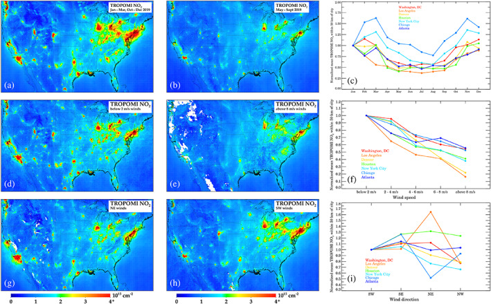
Effects of meteorology and solar zenith angle on column NO2. Top panels show (a) TROPOMI NO2 during the warm season (May–Sept 2019), (b) during the cold season (January–March and October–December 2019), and (c) the monthly variation in seven U.S. cities normalized to January 2019. Middle panels show (d) TROPOMI NO2 when winds are <2 m/s, (e) when winds are >8 m/s, and (f) variations in NO2 as a function of wind speed for seven cities normalized to stagnant conditions. Bottom panels show (g) TROPOMI NO2 when winds are northeasterly, (h) when winds are southwesterly, and (i) variations as a function of wind direction for seven cities normalized to southwesterly winds. Wind variations are using the complete TROPOMI record preceding 1 January 2020 (1 May 2018 to 31 December 2019).
Column NO2 is larger during the cold season than during the warm season over the majority of our domain, despite NO x emissions generally peaking during summer months due to a heavy air conditioning load (Abel et al., 2017; He et al., 2013) and more vehicle miles traveled (https://www.transtats.bts.gov/osea/seasonaladjustment/?PageVar=VMT). The larger NO2 concentrations during the winter are instead due to the longer NO2 lifetime during the cold season, primarily due to slower photolysis rates. When NO x is emitted during the warm season, it is transformed into other chemical species, such as O3 and HNO3, more quickly than during the winter. Also, the fraction of NO x that is in the form of NO2 (rather than NO) is variable, largely due to relative levels of O3 and sunlight. We find that in most near‐urban locations column NO2 amounts are 1.5–3 times larger during the winter than during the summer and can vary substantially between city.
In a next step, we account for wind speed and wind direction in the spatiotemporal variation of NO2 columns. In the middle and bottom panels of Figure 1, we demonstrate the effects of wind speed and wind direction on the NO2 in our domain. Increases in wind speed yield NO2 decreases due to quicker dispersion away from the city centers. For example, in New York City, Washington DC, Atlanta, and Chicago, all cities with relatively flat topography and located in the eastern United States, increasing wind speeds from nearly stagnant to >8 m/s decreases NO2 by 30–60%. Conversely, in Denver and Los Angeles, cities with more heterogeneous topography and with general isolation from an agglomeration of cities show a stronger dependence on wind speed; increasing wind speeds from nearly stagnant to >8 m/s decreases NO2 by 70–85%. In both instances, these examples show the strong dependence of wind speed on local NO2 amounts.
Similarly, wind direction has a large role in the local NO2 amounts, although the effects of wind direction are nonlinear. Generally, northwest winds yield the cleanest conditions in most U.S. cities, but the effects of other wind directions are more nuanced. For example, southwesterly winds yield the worst air quality in New York City, while northeasterly winds yield the largest NO2 in Washington, D.C. This is due to the fact that the other city lies upwind in each opposing scenario. Changes in wind direction, given the same wind speed, can yield differences in NO2 in major cities by up to 70%, and must be accounted for if properly attributing NO2 changes to NO x emissions. Climatological patterns for all cities are shown in the supporting information (Figures S2–S4).
While 2‐m air temperature and boundary layer depth may be affecting the NO2 concentrations, these are not independent of the aforementioned factors: solar zenith angle, wind speed, and wind direction. In fact, solar zenith angle, wind speed, and wind direction are by themselves highly skilled predictors of near‐surface temperatures and boundary layer depth in most instances. Since we are focused on mostly clear‐sky days, clouds have limited effects here. Previous day's precipitation may also be a contributing factor to daily NO2 amounts, but in many areas, the wind direction will partially account for this, since northwest winds usually follow large rain events in most areas.
3.2. Effects of COVID‐19 Physical Distancing on NO2
In order to quantify rapid changes in NO x due to COVID‐19 physical distancing, we calculate NO2 changes in North American cities using three different methods and a reference method. The results for all cities are shown in Table 1.
Table 1.
Percentage Drop in Column NO2 as Observed by TROPOMI
| Reference case | Account for solar zenith angle only | Account for solar zenith angle and meteorology | ||||
|---|---|---|---|---|---|---|
| Method 0 | Method 1 | Method 2 | Method 3 | Mean of methods 1–3 | Median of methods 1–3 | |
| City name | Δ between months 2020 only (January–February vs. 15 March to 30 April) | Δ between years 2019 vs. 2020 (15 March to 30 April) | Using ERA5 analogs to account for meteorology 2019 versus 2020 (15 March to 30 April) | Using GEM‐MACH to infer NO2, 2020 only (15 March to 30 April) | ||
| San Jose | 65.2% | 43.4% | 40.7% | 43.5% | 42.5% | 43.4% |
| Los Angeles | 66.1% | 32.6% | 32.5% | 38.6% | 34.6% | 32.6% |
| Toronto | 60.4% | 31.0% | 17.0% | 42.0% | 30.0% | 31.0% |
| Philadelphia | 50.3% | 36.6% | 30.7% | 22.1% | 29.8% | 30.7% |
| Denver | 25.8% | 29.2% | 23.4% | 39.1% | 30.6% | 29.2% |
| Atlanta | 39.6% | 35.2% | 27.4% | 20.2% | 27.6% | 27.4% |
| Detroit | 35.5% | 29.9% | 22.8% | 15.6% | 22.8% | 22.8% |
| Boston | 40.3% | 22.8% | 23.5% | 17.8% | 21.4% | 22.8% |
| Washington DC | 42.9% | 31.4% | 21.2% | 6.7% | 19.8% | 21.2% |
| Montreal | 12.5% | 3.3% | 20.9% | 30.2% | 18.1% | 20.9% |
| New York City | 32.7% | 20.2% | 20.0% | 17.9% | 19.4% | 20.0% |
| New Orleans | 41.7% | 13.5% | 19.6% | 22.5% | 18.5% | 19.6% |
| Las Vegas | 66.7% | 9.5% | 18.4% | 42.0% | 23.3% | 18.4% |
| Houston | 38.9% | 26.3% | 15.6% | 1.9% | 14.6% | 15.6% |
| Chicago | 31.0% | 23.6% | 14.9% | 3.5% | 14.0% | 14.9% |
| Phoenix | 43.9% | 12.8% | 14.8% | 35.4% | 21.0% | 14.8% |
| Austin | 34.3% | 14.5% | 9.4% | 16.1% | 13.3% | 14.5% |
| Dallas | 41.9% | 11.9% | 3.6% | 16.7% | 10.7% | 11.9% |
| Miami | 27.9% | 16.1% | −1.6% | 11.0% | 8.5% | 11.0% |
| Minneapolis | 0.1% | 14.3% | 9.2% | 8.1% | 10.5% | 9.2% |
| Mean of each method | 39.9% | 22.9% | 19.2% | 22.5% | 21.6% | 21.6% |
The reference method, Method 0, compares the prelockdown and postlockdown periods and represents the “true” NO2 change; however, this method does not account for seasonal changes and, thus, is not considered in the medians/means.
In Method 1, we compare an average of 15 March to 30 April 2020 to the same timeframe of 2019. In Figure 2, we show difference and ratio plots between these 2 years (i.e., Method 1). The largest decreases in NO2 are near the major cities in North America. We also find regional decreases in the eastern North America. Conversely, the central and northwestern United States have seen little change between years, which is likely due to the high fraction of NO2 attributed to biogenic sources and long‐range transport. We also observe substantial decreases near retired electricity generating units in the western United States (Storrow, 2019).
Figure 2.
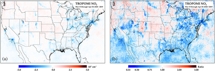
TROPOMI NO2 differences between 2019 and 2020, using 15 March to 30 April 2020 as the post‐COVID‐19 period. Plots are showing (a) the absolute difference and (b) the ratio between years.
In Figure 3, we demonstrate Method 2. Here, we show the 2019 and 2020 28‐day running TROPOMI NO2 medians after accounting for solar zenith angle, day‐of‐week patterns, and two meteorological factors: wind speed and wind direction. A 28‐day period is chosen so as to best average out any random fluctuations not associated with meteorological influences, such as missing data or real changes in NO x emissions due to temperature changes, but there may have been some fluctuations that cannot be averaged out. In Figure 3, the January values are uniformly lower than their true values (Figure S5) because we are normalizing to April meteorological conditions (i.e., solar zenith angle is lower in April as compared to January). In New York City, we calculate a 20.0% drop in NO2 due to COVID‐19 precautions. We find that there is no difference between Method 2—which accounts for meteorology—and Method 1—which only accounts for solar zenith angle. This suggests that varying meteorological conditions in New York City, while different between years, may not have had a strong biasing effect. However, in Washington D.C., we find favorable conditions in 2020 as compared to 2019 because we observe substantially different NO2 drops before (31.4%) and after (21.2%) correcting for the meteorology. These results are corroborated by the wind speed and direction (Figure S6). In 2019, winds were on average southwesterly, while in 2020, winds had more of a northwesterly and therefore cleaner component. Of all cities analyzed, we find that Miami had the most favorable conditions for low NO2 in 2020 as compared to 2019; in 2020, winds were stronger from the south—in this case a cleaner air mass—than in 2019, which had relatively stagnant winds. Conversely, in Montreal, New Orleans, and Las Vegas, meteorological conditions appeared to be unfavorable in 2020 as compared to 2019.
Figure 3.
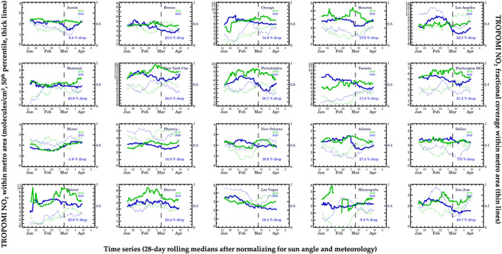
Trends in TROPOMI NO2 since 1 January in 2019 and 2020 after accounting for meteorological variability and solar zenith angle. The thick lines represent the 28‐day rolling median value (50th percentile) in a 0.4° × 0.4° box centered on the city center for the largest cities (New York City, Los Angeles, Chicago, Toronto, and Houston) and 0.2° × 0.2° box in all other cities. The thin lines represent the fractional coverage (0–1) in the coincident spatiotemporal domain.
Meteorological factors that we do not account for in Method 2 are a difference in the number of cloudy scenes and the amount of snow cover between years. In particular, the northern United States had more snow cover in late February and early March in 2019 than in 2020 (Figure S7). In Figure 3, we also show the fractional coverage of the metropolitan area during the 28‐day period. For example, in New York City, there was ~0.6 fractional coverage in early March 2020, while in 2019 there was only ~0.3 fractional coverage during the same timeframe. As a result, some of the higher values during this timeframe may be related to fewer valid pixels in outlying areas, which retain snow for longer, and perhaps a snow‐related reflectivity artifact even though pixels over snow cover are predominantly removed. This is also why some other snow‐prone cities like Chicago, Philadelphia, Toronto, Detroit, Denver, and Minneapolis show large variability preceding March. Beginning in mid‐March, snow cover was largely gone in most U.S. cities during both years.
In Figure 4, we demonstrate Method 3, in which we account for meteorology and chemical interactions using a chemical transport model. We create a theoretical TROPOMI column NO2 using ECCC's regional operational air quality forecast model (Moran et al., 2009; Pendlebury et al., 2018), which accounts for typical seasonal emission changes but not for any impacts due to the COVID‐19 lockdowns; this helps provide expected NO2 levels with a business as usual scenario. Around mid‐March there is often a divergence between the expected and observed NO2 in the major cities. Using this method, largest NO2 reductions due to COVID‐19 precautions are in Toronto, San Jose, and Las Vegas. Similar to Method 2, we find that NO2 changes are generally smaller in the Northeastern United States and Florida as compared to Method 1 after accounting for meteorology. In 15 of the 20 studied cities, we find that Methods 2 and 3, which utilize independent meteorological data sets, show similar biasing effects of meteorology (favorable vs. unfavorable) when compared to Method 1.
Figure 4.
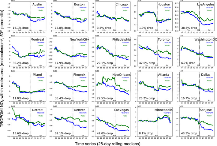
Trends in TROPOMI NO2 since 1 January 2020. The actual observed columns are shown in black, while the “expected” columns—using GEM‐MACH to infer NO2 in the absence of lockdowns—is shown in blue. The lines represent the 28‐day rolling median value (50th percentile) in a 0.4° × 0.4° box centered on the city center for the largest cities (New York City, Los Angeles, Chicago, Toronto, and Houston) and 0.2° × 0.2° box in all other cities.
4. Conclusions and Discussion
We estimate that NO2 adjusted for seasonality and meteorology temporarily dropped between 9–43% in North American cities due to COVID‐19 precautions, with a median drop of 21.6% before and after COVID‐19 physical distancing. If the solar zenith angle is not accounted for, then the median NO2 drop is 39.9%; this represents the true change of NO2 in cities, but is not particularly helpful if parsing out emissions changes. Our reported median drop of 21.6% after accounting for meteorology is marginally lower than the 22.9% in a simple year‐to‐year comparison, which suggests that 2020 meteorology was slightly favorable for lower NO2, although these effects are most pronounced in the Northeastern United States and Florida.
Here we demonstrate two methodologies, Methods 2 and 3, to account for time‐varying effects of meteorology on NO2 concentrations. Although the NO2 concentration is also function of collocated chemical constituents, such as OH, VOCs, and O3, which also vary by year, the numbers reported here are closer to the true change in NO x emissions than NO2 changes in the absence of accounting for meteorology. There are two main advantages for using Methods 2 and 3 to assess rapid changes in NO x as compared to a year‐to‐year comparison of the same month or seasonal period. Year‐over‐year technological improvements in the North America are generally causing NO x emissions to decrease over time (Goldberg, Lu, Oda, et al., 2019; Nopmongcol et al., 2017; Silvern et al., 2019; Zhang et al., 2018), although we find a statistically insignificant NO2 increase of 0.6% in our cities between 2019 and 2020 in the January–February average. Accounting for year‐over‐year changes would be more important if comparing 2020 values to years preceding 2019. There are two U.S. cities, Denver and Philadelphia, which have consistently lower values in 2020 than in 2019 preceding March, using Method 2. While it is conceivable that there may have been policies in these two cities that yielded significantly lower NO x emissions in 2020 versus 2019 preceding March, Method 3 does not corroborate this and further, we do not think the evidence is strong enough to conclude this given the uncertainty related to meteorological conditions unaccounted for, such as snow cover differences between years.
A deficiency of our method is our reliance on a single satellite instrument and algorithm. It is known that the operational TROPOMI NO2 algorithm underestimates tropospheric vertical column NO2 in urban areas due to its reliance on a global model to provide shape profiles for the air mass factor (AMF); investigating the effects of the AMF bias on trends will be the subject of future work. Also, there may be a clear‐sky bias (Geddes et al., 2012) associated with TROPOMI retrievals, but the results presented here are generally consistent with studies using ground monitors over the coincident region (Bekbulat et al., 2020) and the reported CO2 emissions reductions due to COVID‐19 precautions (Le Quéré et al., 2020).
The estimates of NO2 changes using our methods appear to be reasonable given a quick bottom‐up emissions calculation. Initial statistics indicate vehicle miles traveled dropped by ~40% in April 2020 and that many industrial sources dropped modestly ~5–25% due to lockdown exemptions, NO x reductions between 10% and 35% would be expected. San Jose, Los Angeles, and Toronto appear to have reductions at the high end of this range, while Miami, Minneapolis, and Dallas have values near the lowest end; further work will look into why these cities have reductions on the ends of the spectrum. Rapid assessments of NO2 changes—after normalized for seasonal and meteorological factors—can be used to highlight locations that may have had greater changes in activity and better understand the sources contributing to adverse air quality in each city.
Supporting information
Supporting Information S1
Acknowledgments
This work has been supported by NASA through a Rapid Response grant, a Health and Air Quality (HAQ) grant (Award 80NSSC19K0193), and two Atmospheric Composition Modeling and Analysis Program grants. The work has also been supported by the Department of Energy, Office of Fossil Energy. We would also like to acknowledge valuable comments and input during the manuscript preparation from Joanna Joiner and Lok Lamsal of NASA Goddard, Joel Dreessen of Maryland Department of the Environment, Lucas Henneman of Harvard University T.H. Chan School of Public Health, A.R. “Ravi” Ravishankara of Colorado State University, and Michael Moran of Environment and Climate Change Canada.
Goldberg, D. L. , Anenberg, S. C. , Griffin, D. , McLinden, C. A. , Lu, Z. , & Streets, D. G. (2020). Disentangling the impact of the COVID‐19 lockdowns on urban NO2 from natural variability. Geophysical Research Letters, 47, e2020GL089269. 10.1029/2020GL089269
Data Availability Statement
TROPOMI NO2 data can be freely downloaded from the European Space Agency Copernicus Open Access Hub or the NASA EarthData Portal (http://doi.org/10.5270/S5P-s4ljg54). The 100‐m wind and 2‐m surface temperatures from the ERA5 reanalysis can be freely downloaded from the Copernicus Climate Change (C3S) climate data store (CDS) (http://doi.org/10.24381/cds.adbb2d47) The intermediary data used to generate all figures can be found at http://doi.org/10.6084/m9.figshare.12721724. The submitted manuscript has been created by UChicago Argonne, LLC, Operator of Argonne National Laboratory (“Argonne”). Argonne, a U.S. Department of Energy Office of Science laboratory, is operated under Contract DE‐AC02‐06CH11357.
References
References
- Abel, D. W. , Holloway, T. , Kladar, R. M. , Meier, P. , Ahl, D. , Harkey, M. , & Patz, J. (2017). Response of power plant emissions to ambient temperature in the eastern United States. Environmental Science and Technology, 51(10), 5838–5846. 10.1021/acs.est.6b06201 [DOI] [PubMed] [Google Scholar]
- Beirle, S. , Boersma, K. F. , Platt, U. , Lawrence, M. G. , & Wagner, T. (2011). Megacity emissions and lifetimes of nitrogen oxides probed from space. Science, 333(6050), 1737–1739. 10.1126/science.1207824 [DOI] [PubMed] [Google Scholar]
- Beirle, S. , Borger, C. , Dörner, S. , Li, A. , Hu, Z. , Liu, F. , Wang, Y. , & Wagner, T. (2019). Pinpointing nitrogen oxide emissions from space. Science Advances, 5(11), eaax9800. 10.1126/sciadv.aax9800 [DOI] [PMC free article] [PubMed] [Google Scholar]
- Beirle, S. , Platt, U. , Wenig, M. , & Wagner, T. (2003). Weekly cycle of NO2 by GOME measurements: A signature of anthropogenic sources. Atmospheric Chemistry and Physics, 3(6), 2225–2232. 10.5194/acp-3-2225-2003 [DOI] [Google Scholar]
- Bekbulat, B. , Apte, J. S. , Millet, D. B. , Robinson, A. L. , Wells, K. , & Marshall, J. D. (2020). PM2.5 and ozone air pollution levels have not dropped consistently across the US following societal Covid response. Pre‐print. 10.26434/CHEMRXIV.12275603 [DOI]
- Boersma, K. F. , Eskes, H. J. , Richter, A. , de Smedt, I. , Lorente, A. , Beirle, S. , van Geffen, J. H. G. M. , Zara, M. , Peters, E. , van Roozendael, M. , Wagner, T. , Maasakkers, J. D. , van Der, A. R. J. , Nightingale, J. , de Rudder, A. , Irie, H. , Pinardi, G. , Lambert, J. C. , & Compernolle, S. C. (2018). Improving algorithms and uncertainty estimates for satellite NO2 retrievals: Results from the quality assurance for the essential climate variables (QA4ECV) project. Atmospheric Measurement Techniques, 11(12), 6651–6678. 10.5194/amt-11-6651-2018 [DOI] [Google Scholar]
- Copernicus Climate Change Service (C3S) (2017): ERA5: Fifth generation of ECMWF atmospheric reanalyses of the global climate. Copernicus Climate Change Service Climate Data Store (CDS), date of access. https://cds.climate.copernicus.eu/cdsapp#!/home
- de Foy, B. , Wilkins, J. L. , Lu, Z. , Streets, D. G. , & Duncan, B. N. (2014). Model evaluation of methods for estimating surface emissions and chemical lifetimes from satellite data. Atmospheric Environment, 98, 66–77. 10.1016/j.atmosenv.2014.08.051 [DOI] [Google Scholar]
- Dix, B. , Bruin, J. , Roosenbrand, E. , Vlemmix, T. , Francoeur, C. , Gorchov‐Negron, A. , McDonald, B. , Zhizhin, M. , Elvidge, C. , Veefkind, P. , Levelt, P. , & Gouw, J. (2020). Nitrogen oxide emissions from U.S. oil and gas production: Recent trends and source attribution. Geophysical Research Letters, 47, e2019GL085866. 10.1029/2019GL085866 [DOI] [Google Scholar]
- Duncan, B. N. , Lamsal, L. N. , Thompson, A. M. , Yoshida, Y. , Lu, Z. , Streets, D. G. , Hurwitz, M. M. , & Pickering, K. E. (2016). A space‐based, high‐resolution view of notable changes in urban NO x pollution around the world (2005–2014). Journal of Geophysical Research: Atmospheres, 121, 976–996. 10.1002/2015JD024121 [DOI] [Google Scholar]
- ESA (2020a). Air pollution drops in India following lockdown. Retrieved May 4, 2020, from http://www.esa.int/Applications/Observing_the_Earth/Copernicus/Sentinel-5P/Air_pollution_drops_in_India_following_lockdown
- ESA (2020b). Coronavirus: Nitrogen dioxide emissions drop over Italy. Retrieved May 4, 2020, from http://www.esa.int/ESA_Multimedia/Videos/2020/03/Coronavirus_nitrogen_dioxide_emissions_drop_over_Italy
- Geddes, J. A. , Martin, R. V. , Boys, B. L. , & van Donkelaar, A. (2016). Long‐term trends worldwide in ambient NO2 concentrations inferred from satellite observations. Environmental Health Perspectives, 124(3), 281–289. 10.1289/ehp.1409567 [DOI] [PMC free article] [PubMed] [Google Scholar]
- Geddes, J. A. , Murphy, J. G. , O'Brien, J. M. , & Celarier, E. A. (2012). Biases in long‐term NO2 averages inferred from satellite observations due to cloud selection criteria. Remote Sensing of Environment, 124(2), 210–216. 10.1016/j.rse.2012.05.008 [DOI] [Google Scholar]
- Georgoulias, A. K. , van Der, A. R. J. , Stammes, P. , Boersma, K. F. , & Eskes, H. J. (2019). Trends and trend reversal detection in 2 decades of tropospheric NO2 satellite observations. Atmospheric Chemistry and Physics, 19(9), 6269–6294. 10.5194/acp-19-6269-2019 [DOI] [Google Scholar]
- Goldberg, D. L. , Lu, Z. , Oda, T. , Lamsal, L. N. , Liu, F. , Griffin, D. , McLinden, C. A. , Krotkov, N. A. , Duncan, B. N. , & Streets, D. G. (2019). Exploiting OMI NO2 satellite observations to infer fossil‐fuel CO2 emissions from U.S. megacities. Science of The Total Environment, 695, 133805. 10.1016/j.scitotenv.2019.133805 [DOI] [PubMed] [Google Scholar]
- Goldberg, D. L. , Lu, Z. , Streets, D. G. , de Foy, B. , Griffin, D. , McLinden, C. A. , Lamsal, L. N. , Krotkov, N. A. , & Eskes, H. (2019). Enhanced capabilities of TROPOMI NO2: Estimating NO x from North American cities and power plants. Environmental Science & Technology, 53(21), 12,594–12,601. 10.1021/acs.est.9b04488 [DOI] [PubMed] [Google Scholar]
- Griffin, D. , Zhao, X. , McLinden, C. A. , Boersma, F. , Bourassa, A. , Dammers, E. , Degenstein, D. , Eskes, H. , Fehr, L. , Fioletov, V. , Hayden, K. , Kharol, S. K. , Li, S. M. , Makar, P. , Martin, R. V. , Mihele, C. , Mittermeier, R. L. , Krotkov, N. , Sneep, M. , Lamsal, L. N. , Linden, M. , Geffen, J. , Veefkind, P. , & Wolde, M. (2019). High‐resolution mapping of nitrogen dioxide with TROPOMI: First results and validation over the Canadian Oil Sands. Geophysical Research Letters, 46, 1049–1060. 10.1029/2018GL081095 [DOI] [PMC free article] [PubMed] [Google Scholar]
- He, H. , Hembeck, L. , Hosley, K. M. , Canty, T. P. , Salawitch, R. J. , & Dickerson, R. R. (2013). High ozone concentrations on hot days: The role of electric power demand and NO x emissions. Geophysical Research Letters, 40, 5291–5294. 10.1002/grl.50967 [DOI] [Google Scholar]
- Hilboll, A. , Richter, A. , & Burrows, J. P. (2013). Long‐term changes of tropospheric NO2 over megacities derived from multiple satellite instruments. Atmospheric Chemistry and Physics, 13(8), 4145–4169. 10.5194/acp-13-4145-2013 [DOI] [Google Scholar]
- Hilboll, A. , Richter, A. , & Burrows, J. P. (2017). NO2 pollution over India observed from space—The impact of rapid economic growth, and a recent decline. Atmospheric Chemistry and Physics Discussions, 20(2), 1–18. 10.5194/acp-2017-101 [DOI] [Google Scholar]
- Holcombe, M. , & O'Key, S. (2020). Satellite images show less pollution over the US as coronavirus shuts down public places. Retrieved from https://www.cnn.com/2020/03/23/health/us-pollution-satellite-coronavirus-scn-trnd/index.html
- Ialongo, I. , Virta, H. , Eskes, H. , Hovila, J. , & Douros, J. (2020). Comparison of TROPOMI/Sentinel‐5 precursor NO2 observations with ground‐based measurements in Helsinki. Atmospheric Measurement Techniques, 13(1), 205–218. 10.5194/amt-13-205-2020 [DOI] [Google Scholar]
- Kim, S.‐W. W. , Heckel, A. , Frost, G. J. , Richter, A. , Gleason, J. , Burrows, J. P. , McKeen, S. , Hsie, E. Y. , Granier, C. , & Trainer, M. (2009). NO2 columns in the western United States observed from space and simulated by a regional chemistry model and their implications for NO x emissions. Journal of Geophysical Research, 114, D11301. 10.1029/2008JD011343 [DOI] [Google Scholar]
- Krotkov, N. A. , McLinden, C. A. , Li, C. , Lamsal, L. N. , Celarier, E. A. , Marchenko, S. V. , Swartz, W. H. , Bucsela, E. J. , Joiner, J. , Duncan, B. N. , Boersma, K. F. , Veefkind, J. P. , Levelt, P. F. , Fioletov, V. E. , Dickerson, R. R. , He, H. , Lu, Z. , & Streets, D. G. (2016). Aura OMI observations of regional SO2 and NO2 pollution changes from 2005 to 2015. Atmospheric Chemistry and Physics, 16(7), 4605–4629. 10.5194/acp-16-4605-2016 [DOI] [Google Scholar]
- Lamsal, L. N. , Duncan, B. N. , Yoshida, Y. , Krotkov, N. A. , Pickering, K. E. , Streets, D. G. , & Lu, Z. (2015). U.S. NO2 trends (2005–2013): EPA Air Quality System (AQS) data versus improved observations from the Ozone Monitoring Instrument (OMI). Atmospheric Environment, 110(2), 130–143. 10.1016/j.atmosenv.2015.03.055 [DOI] [Google Scholar]
- Laughner, J. L. , & Cohen, R. C. (2019). Direct observation of changing NO x lifetime in North American cities. Science, 366(6466), 723–727. 10.1126/science.aax6832 [DOI] [PMC free article] [PubMed] [Google Scholar]
- Le Quéré, C. , Jackson, R. B. , Jones, M. W. , Smith, A. J. , Abernethy, S. , Andrew, R. M. , De‐Gol, A. J. , Willis, D. R. , Shan, Y. , Canadell, J. G. , & Friedlingstein, P. (2020). Temporary reduction in daily global CO2 emissions during the COVID‐19 forced confinement. Nature Climate Change, 10, 647–653. 10.1038/s41558-020-0797-x [DOI] [Google Scholar]
- Liu, F. , Page, A. , Strode, S. A. , Yoshida, Y. , Choi, S. , Zheng, B. , Lamsal, L. N. , Li, C. , Krotkov, N. A. , Eskes, H. , van Der, A. R. , Veefkind, P. , Levelt, P. F. , Hauser, O. P. , & Joiner, J. (2020). Abrupt declines in tropospheric nitrogen dioxide over China after the outbreak of COVID‐19. Science Advances, 6(28), eabc2992. 10.1126/sciadv.abc2992 [DOI] [PMC free article] [PubMed] [Google Scholar]
- McLinden, C. A. , Fioletov, V. E. , Krotkov, N. A. , Li, C. , Boersma, K. F. , & Adams, C. (2016). A decade of change in NO2 and SO2 over the Canadian Oil Sands as seen from space. Environmental Science and Technology, 50(1), 331–337. 10.1021/acs.est.5b04985 [DOI] [PubMed] [Google Scholar]
- Moran, M. D. , Ménard, S. , Talbot, D. , Huang, P. , Makar, P. A. , Gong, W. , Gravel, S. , Stroud, C. , Zhang, J. & Zheng, Q. (2009). Particulate‐matter forecasting with GEM‐MACH15, A New Canadian Air‐Quality Forecast Model. In Air Pollution Modeling and Its Application XX. Retrieved from http://www.nato.int/science
- NASA (2020). Pandemic before and after: Northeast US 2015–2019 versus 2020. Retrieved from https://airquality.gsfc.nasa.gov/slider/northeast-2020
- Nopmongcol, U. , Alvarez, Y. , Jung, J. , Grant, J. , Kumar, N. , & Yarwood, G. (2017). Source contributions to United States ozone and particulate matter over five decades from 1970 to 2020. Atmospheric Environment, 167(2017), 116–128. 10.1016/j.atmosenv.2017.08.009 [DOI] [Google Scholar]
- Pendlebury, D. , Gravel, S. , Moran, M. D. , & Lupu, A. (2018). Impact of chemical lateral boundary conditions in a regional air quality forecast model on surface ozone predictions during stratospheric intrusions. Atmospheric Environment, 174, 148–170. 10.1016/j.atmosenv.2017.10.052 [DOI] [Google Scholar]
- Plumer, B. , & Popovich, N. (2020). Traffic and pollution plummet as U.S. cities shut down for coronavirus. Retrieved from https://www.nytimes.com/interactive/2020/03/22/climate/coronavirus-usa-traffic.html
- Pope, R. J. , Chipperfield, M. P. , Savage, N. H. , Ordóñez, C. , Neal, L. S. , Lee, L. A. , Dhomse, S. S. , Richards, N. A. D. , & Keslake, T. D. (2015). Evaluation of a regional air quality model using satellite column NO2: Treatment of observation errors and model boundary conditions and emissions. Atmospheric Chemistry and Physics, 15(10), 5611–5626. 10.5194/acp-15-5611-2015 [DOI] [Google Scholar]
- Reuter, M. , Buchwitz, M. , Schneising, O. , Krautwurst, S. , O'Dell, C. W. , Richter, A. , Bovensmann, H. , & Burrows, J. P. (2019). Towards monitoring localized CO2 emissions from space: Co‐located regional CO2 and NO2 enhancements observed by the OCO‐2 and S5P satellites. Atmospheric Chemistry and Physics, 19(14), 9371–9383. 10.5194/acp-19-9371-2019 [DOI] [Google Scholar]
- Shah, V. , Jacob, D. J. , Li, K. , Silvern, R. F. , Zhai, S. , Liu, M. , Lin, J. , & Zhang, Q. (2020). Effect of changing NO x lifetime on the seasonality and long‐term trends of satellite‐observed tropospheric NO2 columns over China. Atmospheric Chemistry and Physics, 20(3), 1483–1495. 10.5194/acp-20-1483-2020 [DOI] [Google Scholar]
- Silvern, R. F. , Jacob, D. J. , Mickley, L. J. , Sulprizio, M. P. , Travis, K. R. , Marais, E. A. , Cohen, R. C. , Laughner, J. L. , Choi, S. , Joiner, J. , & Lamsal, L. N. (2019). Using satellite observations of tropospheric NO2 columns to infer long‐term trends in US NO x emissions: The importance of accounting for the free tropospheric NO2 background. Atmospheric Chemistry and Physics, 19(13), 8863–8878. 10.5194/acp-19-8863-2019 [DOI] [Google Scholar]
- Stavrakou, T. , Müller, J.‐F. , Boersma, K. F. , van Der, A. R. J. , Kurokawa, J. , Ohara, T. , & Zhang, Q. (2013). Key chemical NO x sink uncertainties and how they influence top‐down emissions of nitrogen oxides. Atmospheric Chemistry and Physics, 13(17), 9057–9082. 10.5194/acp-13-9057-2013 [DOI] [Google Scholar]
- Storrow, B . (2019). America's mega‐emitters are starting to close. Retrieved May 15, 2020, from https://www.eenews.net/stories/1060965553/
- Valin, L. C. , Russell, A. R. , & Cohen, R. C. (2013). Variations of OH radical in an urban plume inferred from NO2 column measurements. Geophysical Research Letters, 40, 1856–1860. 10.1002/grl.50267 [DOI] [Google Scholar]
- van Der, A. R. J. , Eskes, H. J. , Boersma, K. F. , Van Noije, T. P. C. , Van Roozendael, M. , De Smedt, I. , Peters, D. H. M. U. , & Meijer, E. W. (2008). Trends, seasonal variability and dominant NO x source derived from a ten year record of NO2 measured from space. Journal of Geophysical Research, 113(D4), 1, D04302–12. 10.1029/2007JD009021 [DOI] [Google Scholar]
- van Geffen, J. H. G. M. , Eskes, H. J. , Boersma, K. F. , Maasakkers, J. D. , & Veefkind, J. P. (2019). TROPOMI ATBD of the total and tropospheric NO2 data products. Retrieved from http://www.tropomi.eu/sites/default/files/files/publicS5P-KNMI-L2-0005-RP-ATBD_NO2_data_products-20190206_v140.pdf
- Veefkind, J. P. , Aben, I. , McMullan, K. , Förster, H. , de Vries, J. , Otter, G. , Claas, J. , Eskes, H. J. , de Haan, J. F. , Kleipool, Q. , van Weele, M. , Hasekamp, O. , Hoogeveen, R. , Landgraf, J. , Snel, R. , Tol, P. , Ingmann, P. , Voors, R. , Kruizinga, B. , Vink, R. , Visser, H. , & Levelt, P. F. (2012). TROPOMI on the ESA Sentinel‐5 precursor: A GMES mission for global observations of the atmospheric composition for climate, air quality and ozone layer applications. Remote Sensing of Environment, 120(2012), 70–83. 10.1016/j.rse.2011.09.027 [DOI] [Google Scholar]
- Wang, C. , Wang, T. , & Wang, P. (2019). The spatial–temporal variation of tropospheric NO2 over China during 2005 to 2018. Atmosphere, 10(8), 444. 10.3390/atmos10080444 [DOI] [Google Scholar]
- Zhang, R. , Wang, Y. , Smeltzer, C. , Qu, H. , Koshak, W. , & Folkert Boersma, K. (2018). Comparing OMI‐based and EPA AQS in situ NO2 trends: Towards understanding surface NO x emission changes. Atmospheric Measurement Techniques, 11(7), 3955–3967. 10.5194/amt-11-3955-2018 [DOI] [Google Scholar]
- Zhang, R. , Zhang, Y. , Lin, H. , Feng, X. , Fu, T.‐M. , & Wang, Y. (2020). NO x emission reduction and recovery during COVID‐19 in East China. Atmosphere, 11(4), 433. 10.3390/atmos11040433 [DOI] [Google Scholar]
- Zhao, X. , Griffin, D. , Fioletov, V. , McLinden, C. , Cede, A. , Tiefengraber, M. , Müller, M. , Bognar, K. , Strong, K. , Boersma, F. , Eskes, H. , Davies, J. , Ogyu, A. , & Lee, S. C. (2020). Assessment of the quality of TROPOMI high‐spatial‐resolution NO2 data products in the Greater Toronto Area. Atmospheric Measurement Techniques, 13(4), 2131–2159. 10.5194/amt-13-2131-2020 [DOI] [Google Scholar]
References From the Supporting Information
- Bey, I. , Jacob, D. J. , Yantosca, R. M. , Logan, J. A. , Field, B. D. , Fiore, A. M. , Li, Q. , Liu, H. Y. , Mickley, L. J. , & Schultz, M. G. (2001). Global modeling of tropospheric chemistry with assimilated meteorology: Model description and evaluation. Journal of Geophysical Research, 106(D19), 23,073–23,095. 10.1029/2001JD000807 [DOI] [Google Scholar]
- Choi, S. , Lamsal, L. N. , Follette‐Cook, M. , Joiner, J. , Krotkov, N. A. , Swartz, W. H. , Pickering, K. E. , Loughner, C. P. , Appel, W. , Pfister, G. , Saide, P. E. , Cohen, R. C. , Weinheimer, A. J. , & Herman, J. R. (2019). Assessment of NO2 observations during DISCOVER‐AQ and KORUS‐AQ field campaigns. Atmospheric Measurement Techniques, 13(5), 2523–2546. 10.5194/amt-13-2523-2020 [DOI] [PMC free article] [PubMed] [Google Scholar]
- Coats, C. J. (1996). High‐performance algorithms in the Sparse Matrix Operator Kernel Emissions (SMOKE) Modeling System, American Meteorological Society, Atlanta, GA. USA, Proceedings of the Ninth AMS Joint Conference on Applications of Air Pollution Meteorology with AWMA.
- Côté, J. , Gravel, S. , Méthot, A. , Patoine, A. , Roch, M. , & Staniforth, A. (1998). The operational CMC–MRB Global Environmental Multiscale (GEM) model. Part I: Design considerations and formulation. Monthly Weather Review, 126(6), 1373–1395. [DOI] [Google Scholar]
- Goldberg, D. L. , Anenberg, S. C. , Mohegh, A. , Lu, Z. , & Streets, D. G. (2020). TROPOMI NO2 in the United States: A detailed look at the annual averages, weekly cycles, effects of temperature, and correlation with PM2.5. 10.1002/essoar.10503422.1 [DOI] [PMC free article] [PubMed]
- Goldberg, D. L. , Lamsal, L. N. , Loughner, C. P. , Swartz, W. H. , Lu, Z. , & Streets, D. G. (2017). A high‐resolution and observationally constrained OMI NO2 satellite retrieval. Atmospheric Chemistry and Physics, 17(18), 11,403–11,421. 10.5194/acp-17-11403-2017 [DOI] [Google Scholar]
- Ialongo, I. , Herman, J. R. , Krotkov, N. , Lamsal, L. N. , Folkert Boersma, K. , Hovila, J. , & Tamminen, J. (2016). Comparison of OMI NO2 observations and their seasonal and weekly cycles with ground‐based measurements in Helsinki. Atmospheric Measurement Techniques, 9(10), 5203–5212. 10.5194/amt-9-5203-2016 [DOI] [Google Scholar]
- Kleipool, Q. L. , Dobber, M. R. , de Haan, J. F. , & Levelt, P. F. (2008). Earth surface reflectance climatology from 3 years of OMI data. Journal of Geophysical Research, 113, D18308. 10.1029/2008JD010290 [DOI] [Google Scholar]
- Lamsal, L. N. , Krotkov, N. A. , Celarier, E. A. , Swartz, W. H. , Pickering, K. E. , Bucsela, E. J. , Gleason, J. F. , Martin, R. V. , Philip, S. , Irie, H. , Cede, A. , Herman, J. , Weinheimer, A. , Szykman, J. J. , & Knepp, T. N. (2014). Evaluation of OMI operational standard NO2 column retrievals using in situ and surface‐based NO2 observations. Atmospheric Chemistry and Physics, 14(21), 11,587–11,609. 10.5194/acp-14-11587-2014 [DOI] [Google Scholar]
- Laughner, J. L. , Zare, A. , & Cohen, R. C. (2016). Effects of daily meteorology on the interpretation of space‐based remote sensing of NO2 . Atmospheric Chemistry and Physics, 16(23), 15,247–15,264. 10.5194/acp-16-15247-2016 [DOI] [Google Scholar]
- Laughner, J. L. , Zhu, Q. , & Cohen, R. C. (2019). Evaluation of version 3.0B of the BEHR OMI NO2 product. Atmospheric Measurement Techniques, 12(1), 129–146. 10.5194/amt-12-129-2019 [DOI] [Google Scholar]
- Lin, J. T. , Liu, M. Y. , Xin, J. Y. , Boersma, K. F. , Spurr, R. , Martin, R. V. , & Zhang, Q. (2015). Influence of aerosols and surface reflectance on satellite NO2 retrieval: Seasonal and spatial characteristics and implications for NO x emission constraints. Atmospheric Chemistry and Physics, 15(19), 11,217–11,241. 10.5194/acp-15-11217-2015 [DOI] [Google Scholar]
- Liu, M. , Lin, J. , Boersma, K. F. , Pinardi, G. , Wang, Y. , Chimot, J. , Wagner, T. , Xie, P. , Eskes, H. , van Roozendael, M. , Hendrick, F. , Wang, P. , Wang, T. , Yan, Y. , Chen, L. , & Ni, R. (2019). Improved aerosol correction for OMI tropospheric NO2 retrieval over East Asia: Constraint from CALIOP aerosol vertical profile. Atmospheric Measurement Techniques, 12(1), 1–21. 10.5194/amt-12-1-2019 [DOI] [Google Scholar]
- Lorente, A. , Folkert Boersma, K. , Yu, H. , Dörner, S. , Hilboll, A. , Richter, A. , Liu, M. , Lamsal, L. N. , Barkley, M. , de Smedt, I. , van Roozendael, M. , Wang, Y. , Wagner, T. , Beirle, S. , Lin, J. T. , Krotkov, N. , Stammes, P. , Wang, P. , Eskes, H. J. , & Krol, M. (2017). Structural uncertainty in air mass factor calculation for NO2 and HCHO satellite retrievals. Atmospheric Measurement Techniques, 10(3), 759–782. 10.5194/amt-10-759-2017 [DOI] [Google Scholar]
- McLinden, C. A. , Fioletov, V. , Boersma, K. F. , Kharol, S. K. , Krotkov, N. , Lamsal, L. , Makar, P. A. , Martin, R. V. , Veefkind, J. P. , & Yang, K. (2014). Improved satellite retrievals of NO2 and SO2 over the Canadian oil sands and comparisons with surface measurements. Atmospheric Chemistry and Physics, 14(7), 3637–3656. 10.5194/acp-14-3637-2014 [DOI] [Google Scholar]
- Palmer, P. I. , Jacob, D. J. , Chance, K. , Martin, R. V. , Spurr, R. J. D. , Kurosu, T. P. , Bey, I. , Yantosca, R. , Fiore, A. , & Li, Q. (2001). Air mass factor formulation for spectroscopic measurements from satellites: Application to formaldehyde retrievals from the Global Ozone Monitoring Experiment. Journal of Geophysical Research, 106(D13), 14,539–14,550. 10.1029/2000JD900772 [DOI] [Google Scholar]
- Russell, A. R. , Perring, A. E. , Valin, L. C. , Bucsela, E. J. , Browne, E. C. , Wooldridge, P. J. , & Cohen, R. C. (2011). A high spatial resolution retrieval of NO2 column densities from OMI: Method and evaluation. Atmospheric Chemistry and Physics, 11(16), 8543–8554. 10.5194/acp-11-8543-2011 [DOI] [Google Scholar]
- Russell, A. R. , Valin, L. C. , Bucsela, E. J. , Wenig, M. O. , & Cohen, R. C. (2010). Space‐based constraints on spatial and temporal patterns of NO x emissions in California, 2005–2008. Environmental Science and Technology, 44(9), 3608–3615. 10.1021/es903451j [DOI] [PubMed] [Google Scholar]
- Stavrakou, T. , Müller, J.‐F. , Bauwens, M. , Boersma, K. F. , & van Geffen, J. (2020). Satellite evidence for changes in the NO2 weekly cycle over large cities. Scientific Reports, 10(1), 10066. 10.1038/s41598-020-66891-0 [DOI] [PMC free article] [PubMed] [Google Scholar]
- van Geffen, J. , Boersma, K. F. , Eskes, H. , Sneep, M. , ter Linden, M. , Zara, M. , & Veefkind, J. P. (2020). S5P TROPOMI NO2 slant column retrieval: Method, stability, uncertainties and comparisons with OMI. Atmospheric Measurement Techniques, 13(3), 1315–1335. 10.5194/amt-13-1315-2020 [DOI] [Google Scholar]
- Williams, J. E. , Folkert Boersma, K. , Le Sager, P. , & Verstraeten, W. W. (2017). The high‐resolution version of TM5‐MP for optimized satellite retrievals: Description and validation. Geoscientific Model Development, 10(2), 721–750. 10.5194/gmd-10-721-2017 [DOI] [Google Scholar]
Associated Data
This section collects any data citations, data availability statements, or supplementary materials included in this article.
Supplementary Materials
Supporting Information S1
Data Availability Statement
TROPOMI NO2 data can be freely downloaded from the European Space Agency Copernicus Open Access Hub or the NASA EarthData Portal (http://doi.org/10.5270/S5P-s4ljg54). The 100‐m wind and 2‐m surface temperatures from the ERA5 reanalysis can be freely downloaded from the Copernicus Climate Change (C3S) climate data store (CDS) (http://doi.org/10.24381/cds.adbb2d47) The intermediary data used to generate all figures can be found at http://doi.org/10.6084/m9.figshare.12721724. The submitted manuscript has been created by UChicago Argonne, LLC, Operator of Argonne National Laboratory (“Argonne”). Argonne, a U.S. Department of Energy Office of Science laboratory, is operated under Contract DE‐AC02‐06CH11357.