Accounting for Solvent Signal Offsets in the Analysis of Interferometric Sedimentation Velocity Data

Summary

Sedimentation velocity analytical ultracentrifugation has reemerged as an important tool in the characterization of biological macromolecules and nanoparticles. The computational analysis of the evolution of the macromolecular concentration profile allows the characterization of many hydrodynamic and thermodynamic properties of the macromolecules and their interactions. The Rayleigh interference optical system is often the detection method of choice, for its usually superior data quality and the wide applicability of refractive index sensitive detection. However, the interference optical system is also sensitive to the redistribution of co-solvent molecules, which are not of primary experimental interest. In principle, their contribution can be eliminated by an exact geometric and compositional match of the sample solution and the reference solution, achieving the complete optical subtraction of unwanted buffer signals. Unfortunately, in practice, this can often not be perfectly achieved for various reasons, leading to signal offsets arising from unmatched sedimentation of solvent components. If unrecognized, this can lead to significant misfit, accompanied by significant errors in the macromolecular sedimentation parameters. In the present work, we describe an approach of computationally accounting for signals from sedimenting buffer components through explicitly modeling their redistribution with Lamm equation solutions, implemented in the software SEDFIT. We demonstrate how this can restore the sedimentation velocity analysis to yield a high quality fit of the data and to provide correct macromolecular sedimentation parameters.

Text for the Table of Contents:

Sedimentation velocity analytical ultracentrifugation has reemerged as an important tool for macromolecular characterization in solution, including their size-distribution and their hydrodynamic and thermodynamic parameters. It is shown how the data analysis model can be extended to account for signal contributions from small molecular weight co-solutes, thereby improving the flexibility and reliability of the method.

Graphical Abstract

Introduction

In the past decade, sedimentation velocity analytical ultracentrifugation (SV) has experienced a renaissance. In part, this was enabled by the abundant computational abilities that allow us to efficiently solve the partial differential equation governing the sedimentation/diffusion process (the Lamm equation, abbreviated in the following LE),^[1–4] and thereby allow us to fully model the rich information contained in the recorded shapes of the sedimentation boundaries. This stimulated the development of new practical strategies and tools that allow for well-controlled experiments with modern instrumentation, ^[5–7] the adaptation of the mathematical model to the specific imperfections of the sedimentation data,^[8–10] and new models that incorporate the complexity of the sample (expressed, for example, in the form of sedimentation coefficient distributions ^[11,12]). This allows routinely to fit SV data to within the level of the noise of data acquisition, and thereby to extract information with exquisite resolution and sensitivity. Many new applications utilize these techniques, including the characterization of the stoichiometry, thermodynamic and kinetic parameters of (multi-)protein interactions ^[2,3,13], the hydrodynamic characterization of the low resolution structure of biomacromolecules and their complexes,^[14,15] the size-distribution of proteins samples,^[11,12] membrane proteins,^[16,17], carbohydrates ^[18,19], the determination of trace aggregate levels in protein therapeutics, ^[6,20,21] as well as systems in supramolecular chemistry, biomaterials and nanoparticles ^[22–24]. For recent reviews, see. ^[25–27]

The present work is aimed at further refining the correspondence of the mathematical model of analysis with the recorded experimental data in order to increase the level of detail and the accuracy of the method. The two most commonly used systems for optically recording the macromolecular concentration profiles of interest are the UV-VIS absorption optical scanner (ABS) ^[28], and the refractive index sensitive Rayleigh laser interferometry (IF) imaging system ^[29]. These two optical systems differ significantly in the properties of the optical signal and the required properties of the sample. By using the ABS system with an appropriate choice of detection wavelength, macromolecular species can be selectively detected that exhibit specific extinction properties. While the selectivity is a great virtue, the ABS system has limitations in the linearity of the signal, in the low time-resolution, and in the moderate signal/noise ratio. This can severely constrain the experimental concentration range of the sample that can be studied. Further, the absorbance detection also excludes the use of buffer components that absorb at the detection wavelength. For the study of unlabeled proteins, for example, this excludes the presence of nucleotides such as ATP, GDP, as well as high concentrations of DTT or β-mercaptoethanol. In contrast, the IF system can be applied if the macromolecules under investigation have no significant extinction between 220 and 800 nm, such as many synthetic polymers or polysaccharides. Further, it offers a high speed of data acquisition enabled by the imaging system, practically unlimited linearity, the ability to resolve steeper gradients, and higher precision (signal/noise ratio is often on the order of 1000:1, 10 fold higher than ABS). For these reasons, absent other special considerations, IF detection is usually the method of choice in our laboratory. More detailed considerations guiding the selection and technical aspects for conducting SV experiments with both the IF and ABS system can be found, for example, in ^[30]. Frequently, the IF and ABS detection are used jointly to offer spectral deconvolution in multi-component samples, for example, in the study of protein/detergent complex,^[16] or the study of multi-protein complexes.^[13]

A key drawback of the IF system is that it cannot selectively monitor the macromolecular redistribution, but instead reports the overall refractive index changes in the solution, including changes resulting from the redistribution of co-solvents, such as buffer salts. In fact, the signals from buffer salts in ordinary phosphate buffered saline solution are an order of magnitude larger than typical signals of the proteins studied. Usually such signal contributions from co-solvents can be optically eliminated by keeping the sample and reference solutions at exactly the same composition (e.g., through the use of equilibrium dialysis or gel permeation chromatography) and loading both solutions with identical geometry (i.e., loading exactly the same volumes into the sectors of the cell assembly ^[8]). Unfortunately, for a variety of reasons, a perfect match may often not be achieved in practice. For example, some protein samples may not be sufficiently stable for the extended period of time of equilibrium dialysis, and/or they may stick to the dialysis tube and gel filtration material. Also, there are some co-solvents typically used at high concentration with high IF signal contributions, which are not well suited for the practical steps of buffer matching. These typically include buffers containing glycerol, detergents, or molar concentrations of salts or denaturants. Often large residual signal offsets are observed in the IF data that arise from imperfect matching. Buffer signal offsets are also encountered and must be addressed when small pipetting errors occur in experiments where limited sample availability prohibits the possibility of repeating the experiment. Clearly, buffer signal offsets must be properly accounted for in order to prevent inaccuracies in the fit and the derived parameter estimates describing the macromolecular properties.

One of the virtues of modern analysis approaches for directly modeling SV data is that no clearly discernable sedimentation boundary is necessary in order to derive sedimentation and diffusion coefficients of the sedimenting species. This enabled, for example, hydrodynamic studies of small peptides and other small molecules.^[31,32] The goal of the present work was, first, to establish that signals from sedimenting buffer salts can be described with high precision by a single species LE solution, second, to extend the LE model of the buffer salts to different concentrations and solution column geometries in the sample and reference sector, and third, to combine this description of buffer salt mismatch signals with the description of the macromolecular sedimentation of interest. We show in the present paper that the so extended model, referred to as the buffer mismatch model (BMM), can appropriately account for both the solvent and the macromolecular signals, and thereby provide more accurate macromolecular sedimentation parameters, even in experimental situations where the IF data would otherwise be un-interpretable.

Materials and Methods

Theory

The Lamm equation (LE) for ideal sedimentation of an initially uniformly distributed species is

$$\frac{\partial c}{\partial t}=-\frac{1}{r}\frac{\partial }{\partial r}\left(cs{w}^2{r}^2-D\frac{\partial c}{\partial r}r\right)$$ (Eq.1)

,^[1] where s and D are the species’ sedimentation and diffusion coefficients, respectively, and c(r,t) is its time-and radial-dependent concentration evolution in a sector-shaped solution column, reaching from meniscus to bottom, rotating with angular velocity ω. At first sight, the application of this equation to the sedimentation of buffer salts as the species of interest seems problematic due to the expected non-ideality of the salt, with its high concentration, dissociation into ions, and their electrostatic interactions. However, we found that the sedimentation data from buffer salts can be extremely well described with this equation, even using a single species LE for multiple different co-solvents (such as phosphate and sodium chloride in PBS buffer). We believe this is simply due to the relatively feature-less profiles generated by the buffer salts. Since the goal of the analysis is reproducibly accounting for the buffer salt signal rather than the characterization of their hydrodynamic and thermodynamic properties, the empirical modeling of all buffer salts with Eq. 1 is entirely sufficient, assigning effective sedimentation and diffusion coefficients s* and D*, which are reproducible, but not the subject of further interpretation. They may also be transformed operationally into a buoyant molar mass M_b* using the Svedberg equation.

One parameter needed for solving Eq. 1 is the initial loading concentration, expressed in signal units as c₀*. This parameter is related to the molar signal increment and therefore the refractive index increment of the low molecular weight co-solute. It can be treated as a fitting parameter, although it may be correlated with s* and D* in the data analysis due to the shallow gradients exhibited by the co-solute. While this is of no consequence (there is usually no correlation with macromolecular parameters) it can be convenient to provide good starting estimates for c₀* to facilitate the minimization during data fitting. To this end, synthetic boundary experiments were performed that allow the more precise determination of s* , D*, and c₀* (see Results section). As shown in ^[33,34], Eq. 1 can also be applied to this configuration using a step-function or an experimental scan as initial condition. (Although the latter is more desirable because it accounts for imperfections in the overlaying process, it is only applicable for single species models in the absence of time-invariant and radial-invariant noise offsets.)

For the analysis of experiments where co-solvents were present in both the sample and the reference sector, since the refractive index increment of the buffer salts is positive, positive signal contributions c_s were assigned for the sample sector, whereas the contributions c_r from the reference sector were subtracted from the signal

$$a_{buf}\left(r,t\right)=c_s\left(r,t,s*,D,m,b\right)-c_r\left(r,t,s{*}^{\prime },D{*}^{\prime },\Delta m,b\right)$$ (Eq. 2)

This allows us to account for different menisci, m and m+Δm, in the sample and reference sector, respectively. Approximate values for the meniscus m and the mismatch Δm can be usually be visually discerned from the experimental data, and graphical estimates be used to initialize the computational optimization ^[9]. Eq. 2 also allows for the potential presence of different effective co-solvent species (s*, D*) and (s*’, D*’), which may arise from a chemical mismatch of the solvents.

In the presence of macromolecules, the total signal is treated as the sum of the buffer signal (Eq. 2) and the macromolecular signal, which, for example, with the c(s) distribution takes the form,

$$a(r,t)=a_{buf}\left(r,t\right)+b_{TI}\left(r\right)+{\beta }_{RI}\left(t\right)+\int c\left(s\right)L_1\left(s_{1}D\left(s\right),r,t\right)ds$$ (Eq. 3)

with L₁ denoting the Lamm equation solution at unit initial signal, the scaling law D(s) (for proteins usually based on 2/3 power-law dependence of sedimentation and molar mass), ^[12,35] and b_TI(r) and β_RI (t) denoting systematic noise contributions of the IF system, which are determined via algebraic noise decomposition ^[36].

Experimental

All the experiments were performed in a Beckman Coulter ProteomeLab-XL-I analytical ultracentrifuge (Palo Alto, CA), following the standard protocols ^[8,30]. Unless otherwise noted, double sector centrifugal cells with 12 mm charcoal-filled epon centerpieces were loaded with 400 μL of sample and reference solution, and sedimented at 50,000 rpm and 20.0 °C. The evolution of the resulting concentration gradient of material in the cell as a function of time and radial position was monitored using Rayleigh interferometric detection (655 nm).

Synthetic boundary experiments of NaCl were carried out with double-capillary-type sector charcoal-filled epon centerpieces, where the two sectors are linked by two capillaries (one at the middle to allow the solution to pass, the other at the top to permit air flow).^[37] The cells were loaded with 100 μL sample (salt solution) with the reference sector filled with 400 μL of water. The samples were centrifuged at 30,000 rpm at 23.0 °C overnight.

For the experiments with protein samples BSA was purchased as lyophilized powder from Sigma Aldrich (St. Louis, MO). This protein was reconstituted in phosphate saline (PBS, Cellgro Invitrogen) as 10 mg/mL stock and dialyzed against the same buffer overnight in order to remove the extra salt. The concentration of the filtered solution was measured by using UV-Vis spectrometer. BSA sample solutions were prepared by mixing the BSA final stock, PBS and 1 M NaCl stock or 10X PBS at calculated volume corresponding with the experimental design.

Data Analysis

BMM data analysis was conducted with the software SEDFIT version 11.72 (sedfitsedphat.nibib.nih.gov). For the analysis of NaCl samples alone, the discrete species model was used, and for the experiments with protein samples the c(s) model was used. For the latter, the first 200 scans were loaded into SEDFIT and analyzed with a c(s) model. The continuous sedimentation coefficient distribution was discretized with 200 s-values between 1.5 – 12 S (0.1–30 was used initially to inspect the presence of small species and large aggregates). Tikhonov Philips regularization (P = 0.68), and both radial- and time-invariant noise decomposition were employed. The meniscus, cell bottom position and the frictional ratio were set as floating parameters. The quality of the fit from the data analysis with and without BMM can be accessed by visual inspection on the residual bitmaps.

The buffer mismatch modeling superimposed to the macromolecular c(s) profile was switched on with the keyboard shortcut control-B. In the resulting parameter box, initial starting guesses for s* , M_b*, and c₀* were entered. When a meniscus mismatch was present, this was first indicated in the parameter box, and an initial estimate for reference meniscus was then entered graphically with the mouse, using a left double-click while the control and shift keys are pressed. (It should be noted that the radial region where air is in one sector and sample in the other can be discerned from the straight diagonal scan regions, with the reference meniscus position approximately at the high end of the diagonal lines and the sample meniscus at the low end of the diagonal lines.) The reference meniscus position is then indicated in the data graph by a pink vertical line. It can be treated as an independent fitting parameter, or the meniscus difference Δm can be fixed.

BMM also allows for a mismatch in buffer salt concentration in the sample and reference sector, implemented as a ratio c₀*(sample side)/ c₀*(reference side). This ratio can be fixed (e.g., to a value of 1.0 for a perfect concentration match after successful equilibrium dialysis) or floated as a fitting parameter. Finally, it allows for completely different buffer sedimentation parameters in the reference sector, expressed as separate parameters s*(reference) and M_b*(reference).

Results

Sedimentation of sodium chloride

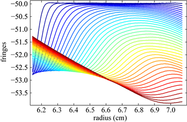
As an initial test for the ability to describe buffer salt signals with single-species LE solutions, we studied the redistribution of NaCl in different configurations. Even though this is not required for the application of BMM, we first show the determination of the sedimentation parameters s* , D*, and c₀* of NaCl in a synthetic boundary experiment. Figure 1A shows initially steep radial profiles (dark blue lines) of the salt signal in the cell around the position of the synthetic boundary, which is followed by diffusive broadening and slight migration towards a virtually linear gradient (dark red lines). This transition happens relatively quickly, similar in time scale to the sedimentation of macromolecules. The rmsd of the fit with a single-species Lamm equation solution, assuming a step-function as initial condition, is 0.0145 fringes. The bitmap representation of the residuals (Figure1B) and the residual plot (Figure 1C) show few diagonal features which might be due to technical imperfections in the data acquisition process (e.g., vibrations of optical elements). Considering the large signal, this is an excellent quality of fit. This demonstrates that the sedimentation of NaCl can be described by the single species Lamm equation model remarkably well.

Figure 1.

Sedimentation profiles of 100 mM NaCl in a synthetic boundary experiment and the best-fit of the Lamm equation solution. (A): Measured time-dependent concentration distributions in the analytical ultracentrifuge in a synthetic boundary experiment (dotted line) at a rotor speed of 30,000 rpm and a rotor temperature of 23 °C using the interference optical detection system. The best-fit of the Lamm equation solution is displayed as solid line. For clarity, the calculated time-invariant noise was subtracted from the data. The color scheme of the curves represents the temporal concentration distribution of the buffer salt, with increasing color temperature (from dark blue to dark red) with time. (B) and (C) display a bitmap representation and an overlay plot of the residuals, respectively. The rmsd is 0.0145 fringes.

The signal in the beginning of the experiment, before the salt diffusion in water represents the change of refractive index corresponding with the loading concentration of the salt, c₀*. In a regular sedimentation configuration, this value is difficult to obtain due to the more shallow profiles and smaller relative concentration difference from meniscus to bottom (Figure 2A). As indicated in Figure1A, we observed 17 fringes increment for the 100 mM NaCl solution, which is approximately five-fold of the signal contribution from the sedimentation of a protein at 1 mg/ml. The estimated apparent sedimentation coefficient and the apparent buoyant mass values are 0.139 S and 89 Da respectively. These values were utilized to initialize the BMM analysis of samples where NaCl was the predominant buffer component (such as in PBS).

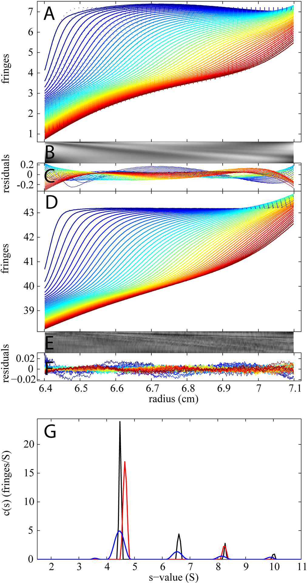
Figure 2.

Signal profiles of NaCl in conventional sedimentation velocity experiments. Panels A, D, and G show the time-dependent evolution of signals (dotted lines) observed in conventional double-sector centerpieces at a rotor speed of 50,000 rpm and a rotor temperature of 20 °C, and the best-fit (solid line) of the Lamm equation solution using the BMM. The representation of the color is the same as described in Figure 1. The systematic time invariant (TI) and radial invariant (RI) noise has been subtracted and every third scan is plotted. (A)-(C) show an experiment with 150 mM NaCl on the sample side and water as a reference. (D)-(F) display the converse experiment with water in the sample sector and 150 mM NaCl in the reference sector. (G)-(I) shows a volume mismatch example with 150 mM NaCl solutions in both sectors, using volumes of 300 μL in the sample sector and 400 μL in the reference sector. The analysis resulted in rmsd of 0.0058, 0.0066 and 0.0086 fringes for the three examples respectively.

Next, Figure 2 shows the sedimentation profiles of NaCl in a double-sector centerpiece with uniform loading concentration in conventional sedimentation velocity experiments at a rotor speed of 50,000 rpm. As can be discerned in Figure 2A, where 150 mM of NaCl is in the sample side with water as reference, even though the profiles are not as steep without the synthetic boundary, we still obtain a signal amplitude of ~2.5 fringes across the cell, corresponding to a relative salt concentration difference from meniscus to bottom of approximately 10%. This generates a very small density gradient aiding the gravitational stability of the sedimentation experiment, but the density gradient is not large enough to significantly affect the buoyancy of the sedimenting macromolecules throughout the sedimentation experiment,^[38] and also not large enough to create significant hydration or other, chemical changes for most proteins. However, if unmatched and unaccounted for, the large scale of the buffer signal would dominate the signal from a macromolecular sedimentation experiment under normal (dilute macromolecular) conditions. Using the estimates regarding c₀* (scaled to the different NaCl concentration), s* and M_b* from the synthetic boundary assay as initial guesses, followed by optimization of these parameters, an excellent fit is obtained with an rmsd of 0.0058 fringes (Figure 2B and 2C).

Figure 2D shows another example of buffer mismatch when water was placed on the sample side and the 150 mM NaCl solution was positioned in reference. Because NaCl is contributing a positive refractive index in the reference, it will be detected with a negative signal. Such a signal would occur, for example, in experiments with excess salt concentration in the reference buffer. Even with this unusual experimental configuration, we can describe the data reliably using BMM, leading to an rmsd of 0.0066 fringes with a Lamm equation solution and its contribution to the overall signal is well accounted for.

Finally, as a last preliminary test of our ability to account for buffer signals alone, we created a geometric mismatch by inserting 150mM NaCl solution at volumes of 400 μL and 300 μL in the reference and sample sector, respectively. The resulting signals are shown in Figure 2G. The BMM can take a geometric mismatch into account by allowing for a meniscus difference between sample and reference. As can be discerned from Figure 2G, this configuration, too, can be described very well with the BMM model. The rmsd of the fit is 0.0086 fringes.

For all three circumstances, BMM allows us to model the distributions well for the buffer salt data with different types of imperfections regarding the buffer match, even for very large mismatch signals. This allows us to proceed with the study of whether we can account for these signals in the presence of macromolecular sedimentation.

Applying BMM to study of protein sedimentation in the presence of buffer mismatch

To this end, we conducted a series of experiments with an identical concentration of BSA in PBS buffer, and created different forms of buffer salt mismatches. The initial input for buffer signal c₀* (scaled to the different NaCl concentration), s* and M_b* were set at values derived from synthetic boundary experiments with NaCl. During the optimization process, the three values were allowed to float. As a reference, Figure 3 shows the data obtained with the standard conditions with buffer virtually perfectly matched in composition and volume between sample and reference cell. Clearly the theoretical boundaries and the sedimentation boundaries superimpose to each other satisfactorily, resulting in a residuals bitmap with very few diagonal features. The root-mean-square deviation for the c(s) model is only 0.0034 fringes. The c(s) peaks are sharp, and reflect monomer and the well-known oligomers.

Figure 3.

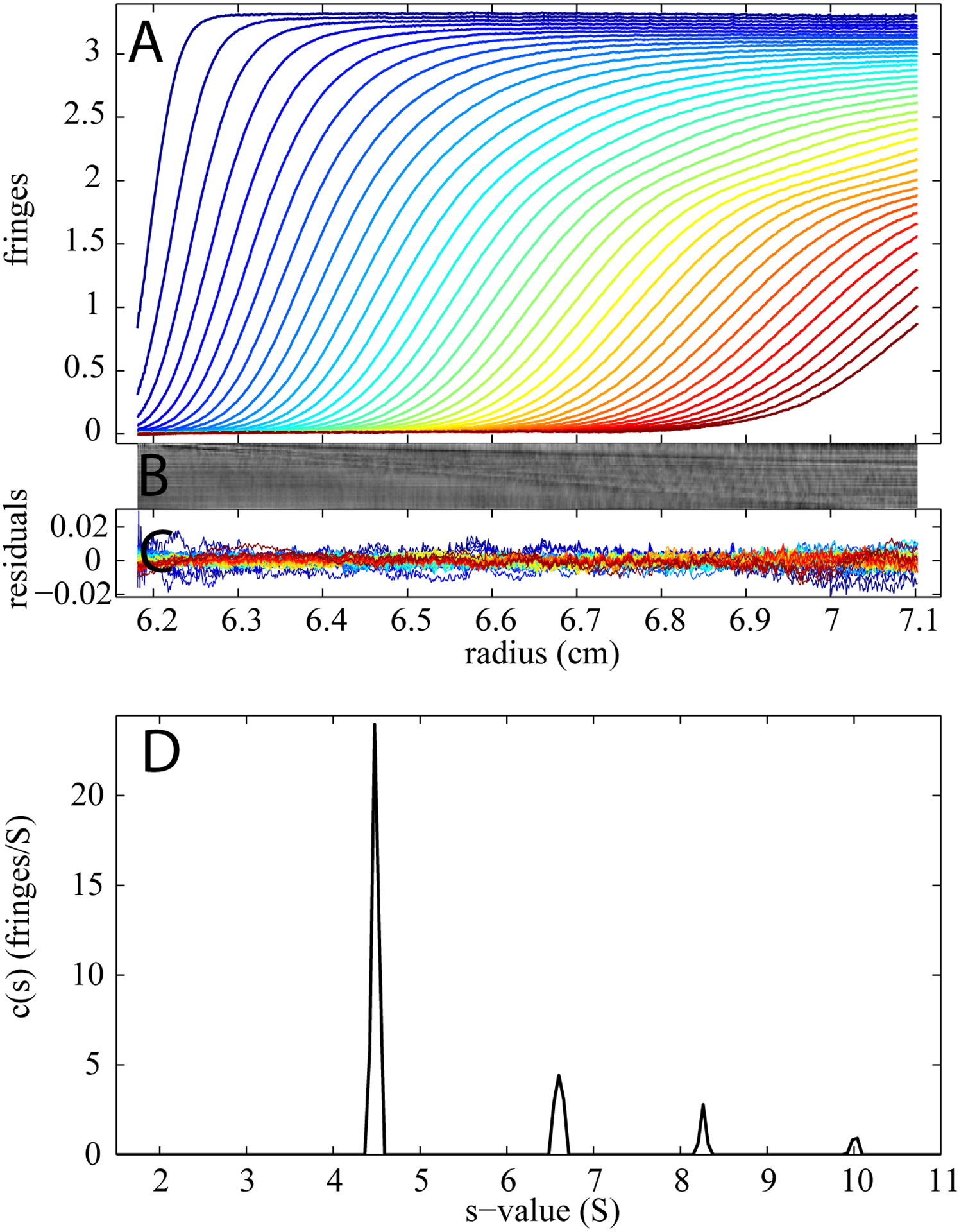
Sedimentation velocity interference profiles of 1 mg/ml BSA in PBS buffer under the standard conditions with buffer virtually perfectly matched in both composition and volume between sample and reference cell. Displayed in panel A are the raw time-dependent radial concentration profiles that were observed at a rotor speed of 50,000 rpm and a rotor temperature of 20°C with interference optics. The systematic TI and RI noise has been subtracted and every fifth scan is plotted. Panel B and C display a bitmap and a residual plot (rmsd = 0.0034 fringes) respectively. Panel D shows the c(s) distribution resulting from the analysis.

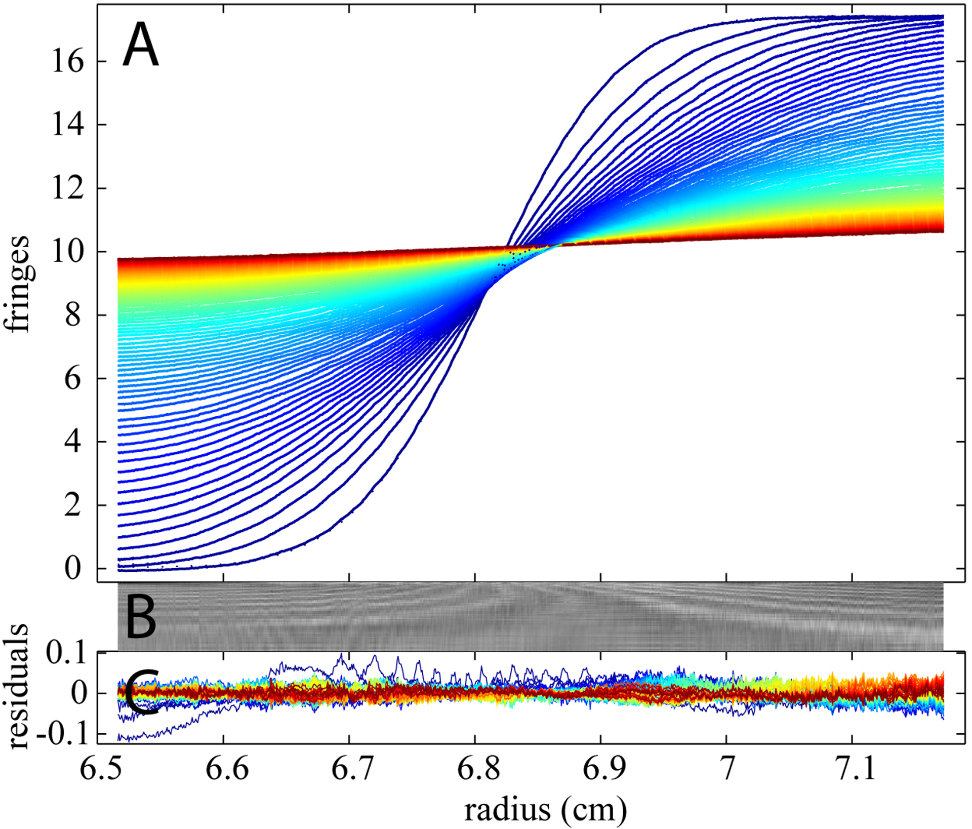
As an example with very strong mismatch signal, we conducted the same experiment with only water in the reference sector (Figure 4). The analysis using the conventional c(s) model without BMM corrections yielded an rmsd of 0.0697 fringes, with visually non-random residuals (Figure 4A–C). The resulting c(s) distribution is shown in panel G as red line, clearly exhibiting incorrect peak positions and peak concentrations (note, for example, the absence of a dimer peak). In contrast, when the BMM was applied to this data set, the best-fit boundaries overlay very well with the measured data (Figure 4D). The residuals bitmaps (4E), plot (4F) and the rmsd (0.0040 fringes) all show striking improvement, indicating a good quality of fit. Moreover the resulting c(s) analysis curve (blue) is highly consistent in peak positions and areas with the one obtained under ‘perfect’ conditions (black). The data only seem to be slightly less informative as indicated by the broader peaks.

Figure 4.

Comparison of the SV analysis with and without BMM of data from 1 mg/ml BSA in PBS with a buffer mismatch. The sample sector contains 300 μL of BSA in PBS and the reference is 400 μL of water. Displayed in panel A are the raw time-dependent radial concentration profiles (dotted line) and the best-fit (solid line) using the conventional c(s) model without BMM. The residual bitmap (B) and the overlay plot (C) indicate the poor quality of the fit (rmsd = 0.0697 fringes). Panel D shows the same data set (dotted line) and the best-fit (solid line) using c(s) model with the BMM correction. Panel E and F display the bitmap and plot of the residuals (rmsd = 0.0040 fringes). For all the analysis, TI and RI noise has been subtracted from the data. Panel G shows the c(s) distributions resulting from both analyses, without BMM correction in red, and after the BMM correction in blue. As a reference, the c(s) distribution from the ‘perfect’ experiment shown in Figure 3 is also included here as a black line.

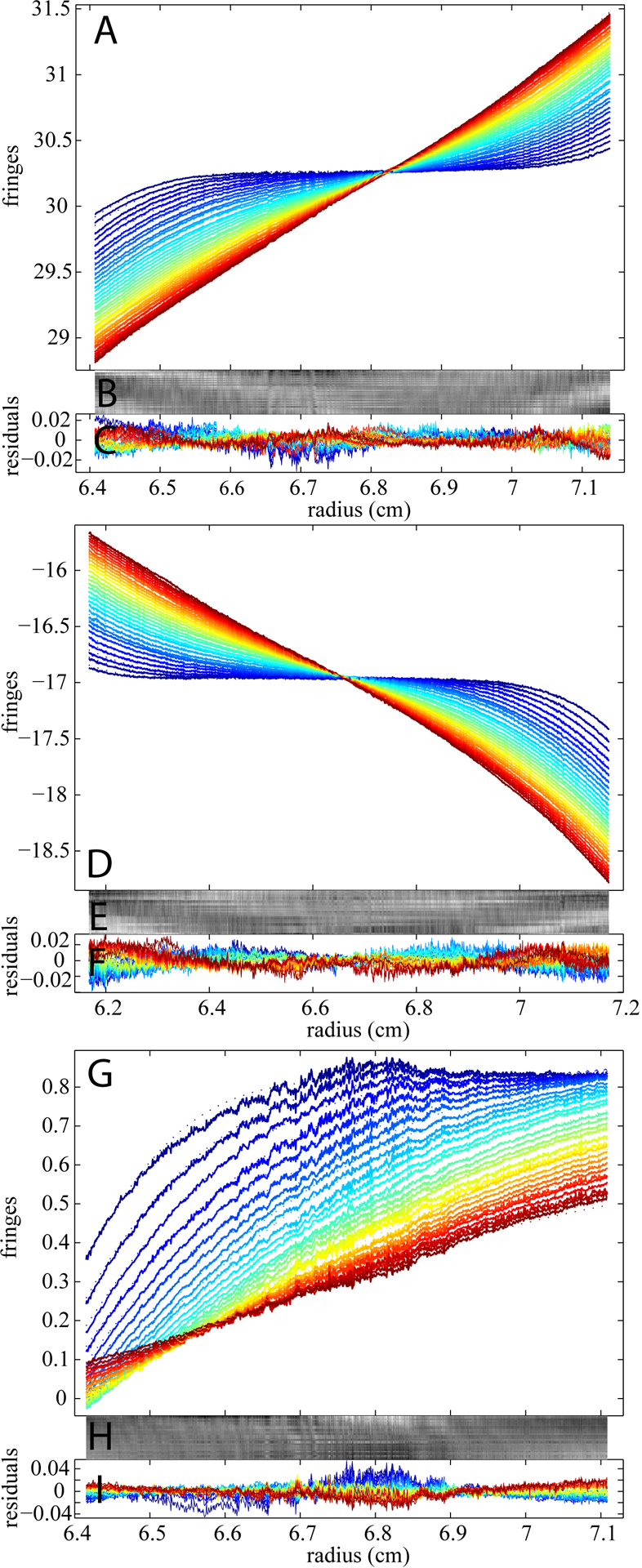
Experiments in different configurations of buffer mismatches are shown in Figure 5. For example, if excess salt is in the reference, the buffer mismatch may significantly obscure the real macromolecular sedimentation signal. This is illustrated in Figure 5A, showing an experiment where BSA in PBS was in the sample sector but 2X PBS in the reference. In contrast, the converse configuration with the extra PBS in the sample side is shown in Figure 5D. Although the studied macromolecule in both samples is BSA (same concentration as the one in Figure 3), the sedimentation boundaries are completely different. Without the BMM, neither of the data sets is interpretable due to the large background of the buffer signal and the resulting rmsd is 0.1870 and 0.0847 fringes for the first and second examples respectively. In contrast, the c(s) model with BMM was able to describe the data well with rmsd values of 0.0042 and 0.0039 fringes, respectively, resulting again in c(s) distributions consisting with those of the reference experiment.

Figure 5.

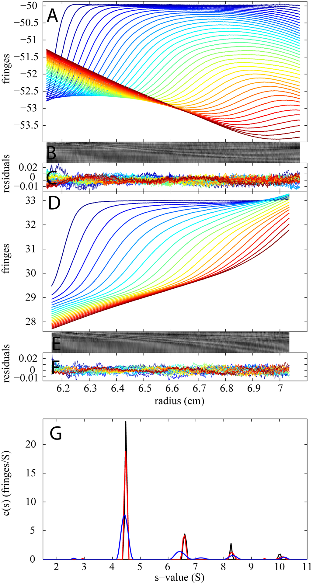
BMM analyses of experimental sedimentation velocity data for 1 mg/ml BSA in PBS buffer with different concentration mismatches. Panel (A) show the data (dotted line) and the best-fit (solid line) for an example with 1 mg/ml BSA in PBS as the sample and 2X PBS as reference. Panel B and C display a bitmap and a residual plot (rmsd = 0.0042 fringes) respectively. Panel (D) displays the data (dotted line) and the best-fit (solid line) for an example with 1 mg/ml BSA in 2 XPBS in the sample cell and PBS in the reference cell. The quality of the fit is shown in residual bitmap (E) and overlay plot (F) (rmsd = 0.0039 fringes). For both analyses, best-fit TI and RI noise contributions have been subtracted from the displayed data. Panel G shows the resulting c(s) distribution: excess concentration of PBS in the reference (red), excess concentration of PBS in the sample (blue), and the ‘perfect’ experiment for comparison (black, same as Figure 3D).

Similar results were obtained in a series of experiments using maltose binding protein as a test macromolecule, when different buffer salt and volume mismatches were applied and the interference optical data acquisition was used. Again, the sedimentation coefficient distributions c(s) calculated with the BMM were in excellent agreement with c(s) results from ‘perfect’ reference experiments without BMM (data not shown).

Finally, we tested the performance of the BMM approach by examining the correspondence between the c(s) distributions when calculated from ABS data or from IF data with BMM. The data in Figure 6 were taken from a study of the ion dependence of the dimerization of the glutamate receptor ligand binding domain GluR6 ^[39]. Due to the high CsCl concentration in this sample, it would be extremely difficult to exactly compensate the large buffer signals arising from the reference and the sample sector. Therefore, a match was not attempted and instead water was filled in the reference sector, to simplify the analysis. This does not affect the ABS data, which are shown in Figure 6A. The IF data, however, are dominated by the large signal from the CsCl sedimentation, and the boundaries from the protein sedimentation cannot be visually discerned (Figure 6D). Both data sets were modeled with a c(s) distribution with and without BMM corrections for the interference and absorbance analysis, respectively. An excellent agreement of the c(s) profiles was observed (Figure 6G).

Figure 6.

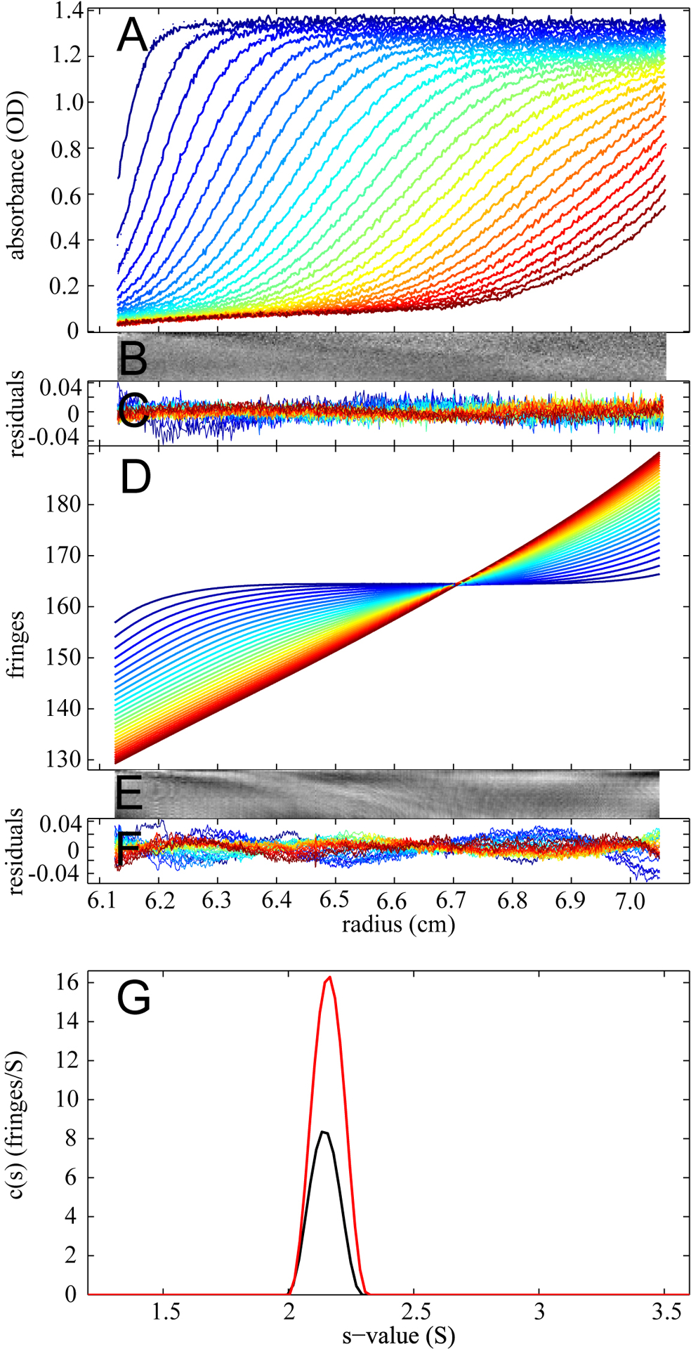
Comparison of the results from absorbance optical and interference optical analysis in the presence of unmatched salt. Data are from the study of a GluR6 mutant ^[39] and show absorbance optical (A-C) and interference optical data (D-F) collected with 27 μM protein, 20 mM HEPES, 2 mM glutamate, and 600 mM CsCl in the sample sector, and water in the reference sector, sedimenting at a rotor speed of 50,000 rpm and a rotor temperature of 20°C. Panel A displays the raw absorbance data at 280 nm (dotted line) and the best-fit resulted from c(s) analysis (solid line). The residual bitmap (B) and the overlay plot (C) represents the quality of the fit (rmsd = 0.0062 OD). Panel D shows the raw interference data (dotted line) and the best-fit resulted from c(s) modeling with the BMM correction. Panel (E) and (F) are the residual bitmap and overlay plot respectively (rmsd = 0.0137 fringes). TI and RI noise has been subtracted from the data. Panel G displays an overlay of the c(s) distribution resulted from analysis of the absorbance data (black) and the interference data (red).

Discussion

The Rayleigh interferometric data acquisition system of the analytical ultracentrifuge has proven extremely valuable for many decades. For example, the data of Figure 6D highlight the remarkable precision of this system, featuring data spanning > 50 fringes that can be fit with a rmsd of 0.014, exhibiting a signal/noise ratio greater than 4,000. However, a significant practical limitation is the requirement for a very precise match of sample volume and chemical composition. Only then will the potentially very large signals arising from the redistribution of small molecular weight buffer components be optically subtracted and eliminated from the recorded IF data. Unfortunately, for many possible reason, this match may not always be possible in practice, rendering the IF signal sometimes seemingly un-interpretable. This can be recognized, for example, from diagonal traces between split sample and reference menisci, curved solution and solvent ‘plateau’ signals, and large systematic residuals when applying the standard models.

The present work addresses this limitation, by showing how the buffer salt signals can be accounted for in the computational analysis of the IF data. This is accomplished by adding to the model for the macromolecular sedimentation of interest a combination of positive and negative signal contributions for the buffer salts in the sample and reference sector, respectively. In our experience with common buffers, the refractive index gradients they produce can be empirically modeled very well with a single discrete Lamm equation solution. The additional parameters introduced can be correlated with each other, but correlate little with the macromolecular parameters of interest. When fitting the additional BMM parameters, we found it useful to enter realistic starting estimates, and only sequentially increase the flexibility of the fit (for example, initially keeping the values for c₀* and Δm fixed).

We have studied the BMM approach in experiments with large compositional and geometric mismatches, which exaggerate the signal contributions over what is often observed from common experimental imperfections. This serves the purpose of demonstrating more clearly the high quality of the description of the signal offsets, and the robustness of the macromolecular parameters derived in their presence. However, in our experience, the BMM performs equally well to account for smaller mismatches, often improving the quality of fit and precision of the results very significantly. For example, signal patterns similar to those shown in Figure 4 may be observed at lower protein concentrations with smaller buffer mismatch, leading to similar bias in the estimated s-values when uncorrected.

An area where higher correlation of the BMM parameters with the macromolecular parameters of interest may occur is the study of small proteins and peptides, which exhibit more shallow macromolecular sedimentation boundaries. This could be a particularly problematic when modeling the data with systems of Lamm equations coupled by chemical reaction kinetics, and/or a priori unknown modes of interaction. Such an approach depends on a detailed analysis of the boundary spread, and the results may be susceptible to experimental imperfections even without buffer mismatch^[3]. This situation could possibly be exacerbated by the additional parameters of BMM. We envision that an alternative two-stage approach we have proposed previously may help to circumvent this difficulty. First, information on the boundary patterns could be extracted from the experimental data with an initial c(s) fit with BMM, leading to isotherm data that could then be modeled with isotherms from effective particle theory ^[40]. Effectively, this avoids interpreting the precise boundary shapes, and therefore the parameter correlation associated with the boundary spread. Of course, where ever possible, the use of multi-signal SV will greatly stabilize any analysis of the interaction of optically distinct components.

In summary, we believe that the BMM approach can significantly extend the utility and flexibility of the IF system, and thereby aid in obtaining more reliable results from sedimentation velocity studies where the IF data acquisition and its rich, high-precision data basis is essential.

References

- [1].Lamm O, Ark. Mat. Astr. Fys 1929, 21B(2), 1–4. [Google Scholar]
- [2].Stafford WF, Sherwood PJ, Biophys Chem 2004, 108, 231–243. [DOI] [PubMed] [Google Scholar]
- [3].Dam J, Velikovsky CA, Mariuzza R, Urbanke C, Schuck P, Biophys J 2005, 89, 619–634. [DOI] [PMC free article] [PubMed] [Google Scholar]
- [4].Brown PH, Schuck P, Comput Phys Commun 2008, 178, 105–120. [DOI] [PMC free article] [PubMed] [Google Scholar]
- [5].Strauss HM, Karabudak E, Bhattacharyya S, Kretzschmar A, Wohlleben W, Coelfen H, Coll. Polym. Sci 2008, 286, 121–128. [DOI] [PMC free article] [PubMed] [Google Scholar]
- [6].Gabrielson JP, Arthur KK, Stoner MR, Winn BC, Kendrick BS, Razinkov V, Svitel J, Jiang Y, Voelker PJ, Fernandes CA, Ridgeway R, Anal Biochem 2009. [DOI] [PubMed] [Google Scholar]
- [7].Arthur KK, Gabrielson JP, Kendrick BS, Stoner MR, J Pharm Sci 2009. [DOI] [PubMed] [Google Scholar]
- [8].Balbo A, Zhao H, Brown PH, Schuck P, J Vis Exp 2009. [DOI] [PMC free article] [PubMed] [Google Scholar]
- [9].Brown PH, Balbo A, Schuck P, Eur Biophys J 2009, 38, 1079–1099. [DOI] [PMC free article] [PubMed] [Google Scholar]
- [10].Gabrielson JP, Arthur KK, Kendrick BS, Randolph TW, Stoner MR, J Pharm Sci 2009, 98, 50–62. [DOI] [PubMed] [Google Scholar]
- [11].Brown PH, Schuck P, Biophys. J 2006, 90, 4651–4661. [DOI] [PMC free article] [PubMed] [Google Scholar]
- [12].Schuck P, Biophys. J 2000, 78, 1606–1619. [DOI] [PMC free article] [PubMed] [Google Scholar]
- [13].Balbo A, Minor KH, Velikovsky CA, Mariuzza R, Peterson CB, Schuck P, Proc Natl Acad Sci U S A 2005, 102, 81–86. [DOI] [PMC free article] [PubMed] [Google Scholar]
- [14].Aragon S, J Comput Chem 2004, 25, 1191–1205. [DOI] [PubMed] [Google Scholar]
- [15].Garcia J Torre de la, Huertas ML, Carrasco B, Biophys J 2000, 78, 719–730. [DOI] [PMC free article] [PubMed] [Google Scholar]
- [16].Salvay AG, Santamaria M, LeMaire M, Ebel C, J Biol. Phys 2007, 33, 399–419. [DOI] [PMC free article] [PubMed] [Google Scholar]
- [17].le Maire M, Arnou B, Olesen C, Georgin D, Ebel C, Moller JV, Nat Protoc 2008, 3, 1782–1795. [DOI] [PubMed] [Google Scholar]
- [18].Harding SE, Carbohydr Res 2005, 340, 811–826. [DOI] [PubMed] [Google Scholar]
- [19].Pavlov GM, Eur Phys J E Soft Matter 2007, 22, 171–180. [DOI] [PubMed] [Google Scholar]
- [20].Berkowitz SA, AAPS J 2006, 8, E590–605. [DOI] [PMC free article] [PubMed] [Google Scholar]
- [21].Brown PH, Balbo A, Schuck P, Aaps J 2008, 10, 481–493. [DOI] [PMC free article] [PubMed] [Google Scholar]
- [22].Coelfen H, Tirosh S, Zaban A, Langmuir 2003, 19, 10656–10659. [Google Scholar]
- [23].Rasa M, Schubert US, Soft Matter 2006, 2, 561–572. [DOI] [PubMed] [Google Scholar]
- [24].O’Neil CP, van der Vlies AJ, Velluto D, Wandrey C, Demurtas D, Dubochet J, Hubbell JA, J Control Release 2009, 137, 146–151. [DOI] [PubMed] [Google Scholar]
- [25].Howlett GJ, Minton AP, Rivas G, Curr Opin Chem Biol 2006, 10, 430–436. [DOI] [PubMed] [Google Scholar]
- [26].Schuck P. In Protein Interactions: Biophysical Approaches for the study of complex reversible systems; Schuck P, Ed.; Springer: New York, 2007; pp 469–518. [Google Scholar]
- [27].Cole JL, Lary JW, T PM, Laue TM, Methods Cell Biol 2008, 84, 143–179. [DOI] [PMC free article] [PubMed] [Google Scholar]
- [28].Hanlon S, Lamers K, Lauterbach G, Johnson R, Schachman HK, Arch. Biochem. Biophys 1962, 99, 157–174. [DOI] [PubMed] [Google Scholar]
- [29].Richards EG, Schachman HK, J. Phys. Chem 1959, 63, 1578–1591. [Google Scholar]
- [30].Brown PH, Balbo A, Schuck P, Curr Protoc Immunol 2008, Chapter 18, Unit 18 15. [DOI] [PubMed]
- [31].Schuck P, MacPhee CE, Howlett GJ, Biophys. J 1998, 74, 466–474. [DOI] [PMC free article] [PubMed] [Google Scholar]
- [32].Pavlov GM, Korneeva EV, Smolina NA, Schubert US, Eur Biophys J 2009. [Google Scholar]
- [33].Cox DJ, Science 1966, 152, 359–361. [DOI] [PubMed] [Google Scholar]
- [34].Schuck P, Biophys. J 1998, 75, 1503–1512. [DOI] [PMC free article] [PubMed] [Google Scholar]
- [35].Schuck P, Perugini MA, Gonzales NR, Howlett GJ, Schubert D, Biophys J 2002, 82, 1096–1111. [DOI] [PMC free article] [PubMed] [Google Scholar]
- [36].Schuck P, Demeler B, Biophys. J 1999, 76, 2288–2296. [DOI] [PMC free article] [PubMed] [Google Scholar]
- [37].Hersh R, Schachman HK, J Am Chem Soc 1955, 77, 5228–5234. [Google Scholar]
- [38].Schuck P, Biophys. Chem 2004, 108, 187–200. [DOI] [PubMed] [Google Scholar]
- [39].Chaudhry C, Plested AJ, Schuck P, Mayer ML, Proc Natl Acad Sci U S A 2009, 106, 12329–12334 [DOI] [PMC free article] [PubMed] [Google Scholar]
- [40].Schuck P. Biophys. J 2010, 98(8) in press [DOI] [PMC free article] [PubMed] [Google Scholar]