

Abstract
Panel data, also known as longitudinal data, consist of a collection of time series. Each time series, which could itself be multivariate, comprises a sequence of measurements taken on a distinct unit. Mechanistic modeling involves writing down scientifically motivated equations describing the collection of dynamic systems giving rise to the observations on each unit. A defining characteristic of panel systems is that the dynamic interaction between units should be negligible. Panel models therefore consist of a collection of independent stochastic processes, generally linked through shared parameters while also having unit-specific parameters. To give the scientist flexibility in model specification, we are motivated to develop a framework for inference on panel data permitting the consideration of arbitrary nonlinear, partially observed panel models. We build on iterated filtering techniques that provide likelihood-based inference on nonlinear partially observed Markov process models for time series data. Our methodology depends on the latent Markov process only through simulation; this plug-and-play property ensures applicability to a large class of models. We demonstrate our methodology on a toy example and two epidemiological case studies. We address inferential and computational issues arising due to the combination of model complexity and dataset size. Supplementary materials for this article are available online.
Keywords: Likelihood, Longitudinal data, Nonlinear dynamics, Particle filter, Sequential Monte Carlo
1. Introduction
Analyzing time series data on a collection of related units provides opportunities to study aspects of dynamic systems—their replicability, or dependence on properties of the units—that cannot be revealed from measurements on a single unit. The units might be individual humans or animals, in an observational or experimental study. The units might also be spatial locations, giving a panel representation of spatiotemporal data. As a consequence of advances in data collection, scientists investigating dynamic systems have growing capabilities to obtain measurements of increasing length on increasingly many units. Statistical investigation of such data, known as panel data analysis, is therefore playing a growing role in the scientific process.
Mechanistic modeling of a dynamic system involves writing down equations describing the evolution of the system through time. Time series analysis using mechanistic models involves determining whether the model provides an adequate description of the system, and if so, identifying plausible values for unknown parameters (Bretó et al. 2009). Stochasticity, nonlinearity and noisy incomplete observations are characteristic features of many systems in the biological and social sciences (Bjørnstad and Grenfell 2001; Dobson 2014). Monte Carlo inference approaches have been developed that are effective for general classes of models with these properties. Such methods include iterated filtering (Ionides, Bretó, and King 2006; Ionides et al. 2015), particle Markov chain Monte Carlo (Andrieu, Doucet, and Holenstein 2010) and synthetic likelihood (Wood 2010). All these inference algorithms obtain their general applicability by enjoying the plug-and-play property, that is, they interface with the dynamic model only through simulation (Bretó et al. 2009; He, Ionides, and King 2010). However, these methodologies do not address the particular structure of panel models and the high-dimensional nature of panel data. Therefore, new methodology is required to analyze panel data when there is a need to consider models outside the linear, Gaussian paradigm. We proceed by building on the iterated filtering approach of Ionides et al. (2015), deriving a panel iterated filtering likelihood maximization algorithm. The panel iterated filtering algorithm, an associated convergence theorem, and a software implementation equipped with an appropriate domain-specific modeling language, all extend the existing theory and practice of iterated filtering.
Across the broad applications of nonlinear partially observed stochastic dynamic models for time series analysis (Douc, Moulines, and Stoffer 2014) one can anticipate many situations where multiple time series are available and give rise to the structure of panel data. In particular, panel data on dynamic systems arises in pharmacokinetics (Donnet and Samson 2013), molecular biology (Chen et al. 2016), infectious disease transmission (Cauchemez et al. 2004; Yang et al. 2010, 2012), and microeconomics (Heiss 2008; Bartolucci, Farcomeni, and Pennoni 2012; Mesters and Koopman 2014). Our methodology differs from those employed by these authors in that it provides plug-and-play likelihood-based inference applicable to general nonlinear, non-Gaussian models. This scope of applicability also sets our goals apart from the extensive panel methodology literature building on a linear regression framework (e.g., Hsiao 2014).
In Section 2, we present a basic panel iterated filtering algorithm, and in Section 3, we prove its convergence under appropriate regularity conditions. An issue arising for large panel datasets is scalability of statistical methodology, and we develop three techniques to address this issue in Sections 4.1–4.3. These scaling techniques are illustrated on a toy example in Section 5. Two scientifically motivated examples follow: modeling the transmission of polio in Section 6, and dynamic variation in human sexual contact rates in Section 7. In Section 8, we conclude by discussing relationships to other approaches and indicating some extensions.
2. Inference Methodology: Panel Iterated Filtering (PIF)
Units of a panel are labeled {1, 2, … , U}, which we write as 1: U. The Nu measurements collected on unit u are written as where is collected at time tu,n with tu,1 < tu,2 < ⋯ < tu,Nu. These data are considered fixed and modeled as a realization of an observable stochastic process Yu,1:Nu. This observable process is constructed to be dependent on a latent Markov process {Xu(t), tu,0 ≤ t ≤ tu,Nu}, for some tu,0 ≤ tu,1. Further requiring that {Xu(t)} and {Yu,i, i ≠ n} are independent of Yu,n given Xu(tu,n), for each n ∈ 1 : Nu, completes the structure required for a partially observed Markov process (POMP) model for unit u (Ionides et al. 2011; King, Nguyen, and Ionides 2016). If all units are modeled as independent, the model is called a PanelPOMP Although we can treat time as either continuous or discrete, our attention will focus on the latent process at the observation times, so we write Xu,n = Xu(tu,n). We suppose that Xu,n and Yu,n take values in arbitrary spaces and , respectively. We suppose that the joint density of Xu,0:Nu and Yu,1:Nu exists, with respect to some suitable measure, and is written as fXu,0:NuYu,1:Nu (xu,0:Nu, yu,1:Nu; θ), with dependence on an unknown parameter . Each component of the vector θ may affect one, several or all units. This framework encompasses fixed effects (discussed in Section 4.2) and random effects (discussed in Section 8). The transition density fXu,n|Xu,n−1 (xu,n | xu,n−1; θ) and measurement density fYu,n|Xu,n (yu,n | xu,n; θ) are permitted to depend arbitrarily on u and n, allowing nonstationary models and the inclusion of covariate time series (illustrated in Section 6). The framework also includes continuous-time dynamic models (illustrated in Section 7) and discrete-time dynamic models (illustrated in Sections 5 and 6), for which Xu,0:Nu is specified directly without ever defining {Xu(t), tu,0 ≤ t ≤ tu,Nu}.
The marginal density of Yu,1:Nu at yu,1:Nu is fYu,1:Nu (yu,1:Nu ; θ) and the likelihood function for unit u is . The likelihood for the entire panel is , and any solution is a maximum likelihood estimate (MLE).
Algorithm PIF.
Panel iterated filtering
| input: |
| Simulator of initial density, fXu,0 (xu,0; θ) for u in 1: U |
| Simulator of transition density, fXu,n|Xu,n−1 (xu,n | xu,n−1 ; θ) for u in 1 : U, n in 1 : Nu |
| Evaluator of measurement density, fYu,n|Xu,n (yu,n | xu,n ; θ) for u in 1 : U, n in 1 : Nu |
| Data, for u in 1 : U and n in 1 : Nu |
| Number of iterations, M |
| Number of particles, J |
| Starting parameter swarm, for j in 1: J |
| Simulator of perturbation density, hu,n(θ | φ ; σ) for u in 1: U, n in 0 : Nu |
| Perturbation sequence, σm for m in 1 : M |
| output: |
| Final parameter swarm, for j in 1: J |
| For m in 1 : M |
| Set for j in 1: J |
| For u in 1 : U |
| Set for j in 1 : J |
| Set for j in 1 : J |
| For n in 1 : Nu |
| for j in 1 : J |
| for j in 1 : J |
| for j in 1 : J |
| Draw k1:J with for i, j in 1 : J |
| and for j in 1 : J |
| End For |
| Set for j in 1: J |
| End For |
| Set for j in 1: J |
| End For |
The PIF algorithm, represented by the pseudocode above, is an adaptation of the IF2 algorithm (Ionides et al. 2015) to PanelPOMP models. Like previous iterated filtering algorithms (Ionides, Bretó, and King 2006; Ionides et al. 2015), PIF explores the space of unknown parameters by stochastically perturbing them and applying sequential Monte Carlo to filter the data seeking for parameter values that are concordant with the data. Perturbations are successively diminished over repeated filtering iterations, leading to convergence to an MLE. This general approach of iterated filtering needs some adaptation in order for it to be useful for PanelPOMP models.
The number of computations required for PIF has order , where N is the mean of {N1, … , NU} and J and M are the number of particles and iterations, defined in the pseudocode. The pseudocode specifies unique labels for each quantity constructed to clarify the logical structure of the algorithm, and a literal implementation of this pseudocode therefore requires storing particles. Each particle contains a perturbed parameter vector and so has size if dim(Θ) is , leading to a total storage requirement of . However, we only need to store the value of the latent process particles, and , and perturbed parameter particles, and , for the current unit, time point and PIF iteration. Taking advantage of this memory over-writing opportunity leads to a storage requirement that is .
The theoretical justification of PIF is based on the observation that a PanelPOMP model can be represented as a time-inhomogeneous POMP model. Algorithms for PanelPOMPs, and their theoretical support, can therefore be derived from previous approaches for POMPs. Here, we use a representation concatenating the time series for each unit, corresponding to a latent POMP process
| (1) |
where is a cumulative latent POMP process time for all panel units up to unit u, given by
| (2) |
and . We leave X(t) undefined for to provide a formal separation between the latent processes for each unit. In (2) we have set the value of this time separation to one, though any positive number would suffice and the exact value is irrelevant on the discrete timescale consisting of the sequence of observation times. In the language of data manipulation, our representation converts wide panel data into a tall format (Wickham 2014). As we show subsequently, a POMP representation using a tall format preserves the theoretical justification for iterated filtering, while also taking advantage of favorable sequential Monte Carlo (SMC) stability properties for long time series. Conversely, a wide format POMP representation risks encountering the curse of dimensionality for SMC (Bengtsson, Bickel, and Li 2008).
This POMP representation of a PanelPOMP model is one of three noted by Romero-Severson et al. (2015) and discussed further in the supplement (Section S1). Romero-Severson et al. (2015) used a different algorithm—their approach was convenient to code and sufficient for their example but its computational feasibility quickly breaks down as the length of each panel time series increases so it is infeasible in situations such as our polio example in Section 6.
3. Convergence of PIF
PIF investigates the parameter space using a particle swarm . With a sufficiently large number J of particles, each iteration m of PIF approximates a Bayes map that selects a particle j with probability proportional to the value of the likelihood function at . Heuristically, repeated application of the Bayes map favors particles with high likelihood and should lead to convergence of the particle swarm to a neighborhood of the MLE. We state such a convergence theorem, followed by the technical assumptions we use to prove it.
Our theorem combines Theorems 1 and 2 of Ionides et al. (2015) in the context of the POMP representation of a PanelPOMP model in (1). Their Theorem 1 proved the existence of a limit distribution for an iterated perturbed Bayes map by taking advantage of its linearity under the Hilbert projective metric. In addition, they showed that sequential Monte Carlo can provide a uniform approximation of this limit distribution. Their Theorem 2 bounded excursion probabilities under this iterated perturbed Bayes map to derive sufficient conditions for the limit distribution to concentrate around the MLE. Here, we combine these two theorems into a simpler statement.
Theorem 1. Let be the output of PIF, with fixed perturbations σm = δ. Suppose regularity conditions A1–A6. For all ϵ > 0, there exists δ, M0 and C such that, for all M ≥ M0 and all j ∈ 1: J,
| (3) |
To discuss the regularity conditions, we need to set up some more notation. We write Y = (Y1,1:N1, … , YU,1:NU) and consequently we write y* for a vector of the entire panel dataset. The likelihood function is ℓ(θ) = fY(y* ; θ) and we suppose the following regularity condition:
-
(A1)
There is a unique MLE, and ℓ(θ) is continuous in a neighborhood of this MLE.
To allow us to talk about parameter perturbations, we define a perturbed parameter space,
for which we write as
| (4) |
For compatibility with the POMP representation of a PanelPOMP in (1), perturbed parameters for each time point and each unit are concatenated in (4) with θu,n being a perturbed parameter for the nth observation on unit u. On the perturbed parameter space , the extended likelihood function is defined as
| (5) |
We suppose that the extended likelihood has a Lipschitz continuity property:
-
(A2)Set , so that . Write for the nth of the terms in (4), so that . There is a C1 such that
(6)
We also assume a uniformly positive measurement density:
-
(A3)There are constants C2 and C3 such that
for all u ∈ 1 : U, n ∈ 1 : Nu, and θ ∈ Θ.
This condition will usually require Θ and to be compact, for all u ∈ 1 : U. Compactness of Θ is satisfied if there is some limit to the scientifically plausible values of each parameter. Compactness of may not be satisfied in practice, but much previous theory for SMC has used this strong requirement (e.g., Del Moral and Guionnet 2001; Le Gland and Oudjane 2004). The remaining conditions concern the perturbation transition density, hu,n(θ | φ ; σ). We suppose that hu,n(θ | φ ; σ) has bounded support on a normalized scale via the following condition:
-
(A4)
There is a C4 such that hu,n(θ | φ ; σ) = 0 when |θ − φ| < C4σ for all u ∈ 1: U, n ∈ 1: Nu and σ.
We also require some regularity of an appropriately rescaled limit of the Markov chain resulting from iterating the perturbation process. Define to be a Markov chain taking values in Θ with drawn uniformly from the starting particles, , and transition density given by
| (7) |
Thus, represents a random-walk-like process corresponding to combining the parameter perturbations of all units and all time points for one iteration of PIF. Now, let {Wσ(t), t ≥ 0} be a right-continuous, piecewise constant process taking values in Θ defined at its points of discontinuity by
| (8) |
If hu,n(θ | φ ; σ) were a scale family of additive perturbations, then would be a random walk that scales to a Brownian diffusion. When Θ has a boundary, cannot be exactly a random walk, but similar diffusion limits can apply (Bossy, Gobet, and Talay 2004). We require that hu,n(θ | φ ; σ) is chosen to be sufficiently regular to have such a diffusion limit, via the following assumptions:
-
(A5)
{Wσ(t), 0 ≤ t ≤ 1} converges weakly as σ → 0 to a diffusion {W(t), 0 ≤ t ≤ 1}, in the space of right-continuous functions with left limits equipped with the uniform convergence topology. For any open set A ⊂ Θ with positive Lebesgue measure and ϵ > 0, there is a δ(A, ϵ) > 0 such that .
-
(A6)
For some t0(σ) and σ0 > 0, Wσ(t) has a positive density on Θ, uniformly over the distribution of W(0) for all t > t0 and σ < σ0.
Proof of Theorem 1. PIF is exactly the IF2 algorithm of Ionides et al. (2015) applied to the POMP representation of a PanelPOMP model in Equation (1). A1 is condition B3 of Ionides et al. (2015) together with a simplifying additional assumption that a unique MLE exists. A2 is a rewriting of their B6. A3 and A4 are essentially their B4 and B5. A5 and A6 match their B1 and B2, respectively. Thus, we have established the conditions used for Theorems 1 and 2 of Ionides et al. (2015) for this POMP representation of a PanelPOMP model. The statement of our Theorem 1 follows directly from these two previous results. □
The perturbation density hu,n(θ | φ ; σ) has usually been chosen to be Gaussian in implementations of the IF2 algorithm and its predecessor, the IF1 algorithm (Ionides, Bretó, and King 2006). The use of Gaussian perturbations requires the user to reparameterize boundaries in the parameter space. This may involve taking a logarithmic transformation of positive parameters and a logistic transform of interval-valued parameters (e.g., see Tables S-3 and S-4). To satisfy assumption A4, Gaussian perturbations must be truncated. Since the Gaussian distribution has short tails, ignoring truncation is practically equivalent to truncation at a large multiple of the standard deviation. Unlike an alternative theoretical framework using Stein’s lemma to approximate derivatives via perturbed parameters and SMC (Doucet, Jacob, and Rubenthaler 2015; Dai and Schön 2016) our justification for PIF does not require the choice of Gaussian perturbations.
4. Scalable Methodology for Large Panels
Theorem 1 provides an asymptotic Monte Carlo convergence guarantee for a dataset of fixed size as the Monte Carlo effort increases. In practice, reaching this Monte Carlo asymptotic regime becomes increasingly difficult as the panel dataset grows, whether the number of units becomes large, or there are many observations per unit, or both. In this section, we consider some techniques that become important when using PIF for big datasets. We demonstrate the methodology on a toy model in Section 5. Subsequently, we demonstrate data analysis for mechanistic panel models using PIF via two examples, one investigating disease transmission of polio and another investigating dynamics of human sexual behavior.
4.1. Monte Carlo Adjusted Profile (MCAP) Confidence Intervals
PIF provides a Monte Carlo approach to maximizing the likelihood function for a PanelPOMP model. It is based on an SMC algorithm that can also provide an unbiased estimate of the maximized likelihood. Monte Carlo methods to evaluate and maximize the likelihood function provide a foundation for constructing confidence intervals via profile likelihood. When computational resources are sufficient to make Monte Carlo error small, its role in statistical inference may be negligible. With large datasets and complex models, we cannot ignore Monte Carlo error so instead we quantify it and draw statistical inferences that properly account for it. We use the Monte Carlo adjusted profile (MCAP) methodology of Ionides et al. (2017) which fits a smooth curve through Monte Carlo evaluations of points on a profile log-likelihood. MCAP then obtains a confidence interval using a cutoff on this estimated profile that is enlarged to give proper coverage despite Monte Carlo uncertainty in its construction. Monte Carlo variability in maximizing and evaluating the likelihood both lead to expected underestimation of the maximized log-likelihood. Despite such bias the MCAP methodology remains valid as long as this likelihood shortfall is slowly varying as a function of the profiled parameter (Ionides et al. 2017). Our toy example in Section 5 demonstrates this phenomenon. For our subsequent examples, we applied the MCAP methodology described by Ionides et al. (2017) and demonstrated in several recent scientific analyses (Smith, Ionides, and King 2017; Ranjeva et al. 2017, 2018; Pons-Salort and Grassly 2018). We used the R implementation of MCAP from Ionides et al. (2017) with an algorithmic smoothing parameter λloess = 0.9 determining the fraction of profile points used to construct the neighborhoods for locally weighted quadratic regression smoothing.
4.2. Unit-Specific Parameters and Marginal Maximization
The parameter space for a PanelPOMP model may be structured into unit-specific and shared parameters. To do this, we introduce a decomposition Θ = Φ × ΨU and θ = (ϕ, ψ1, ψ2, … , ψU) with the joint distribution of Xu,0:Nu and Yu,1:Nu, for each unit u, depending only on the shared parameter and the unit-specific parameter . The general PanelPOMP specification does not insist on the existence of unit-specific parameters. Correspondingly, the PIF algorithm does not require this structure and it does not play a role in the general theory. However, when it exists, we can use this additional structure to advantage within the general framework of PIF. One consequence of the presence of unit-specific parameters arises in a natural structure for the PIF perturbation densities: when PIF is filtering through panel unit u, only unit-specific parameters corresponding to unit u need to be perturbed. Another consequence is the existence of a block structure to the parameter space that can be exploited, as follows.
When U is large, dim(Θ) = dim(Φ) + Udim(Ψ) also becomes large. For a fixed value of ϕ, the marginal likelihoods of ψ1:U can be maximized separately, due to independence between units. Formally, application of iterated filtering to each of these marginal optimizations is a special case of the PIF algorithm with U = 1. Thus, the convergence theory for PIF gives us freedom to alternate marginal optimization steps with joint optimization over Θ, following a block coordinate ascent approach. In practice, we demonstrate a simple two-step algorithm which first attempts to optimize over Θ and then refines the resulting estimates of the unit-specific parameters by marginal searches for each unit. Figure 1 of Section 5 shows that this leads to considerable Monte Carlo variance reduction on an analytically tractable example.
Figure 1.
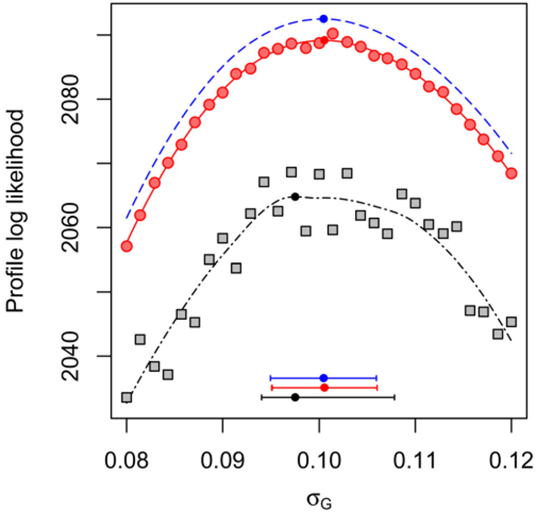
Profile log-likelihood of σG for a panel of size U = 50 for the Gompertz model. Blue line (dashes): exact profile. Red points and line (circles): profile computed with PIF, including marginal maximization for unit-specific parameters. Black points and line (squares): profile computed with PIF using onlyjoint maximization. The horizontal bars show 95% MCAP confidence intervals with a small filled circle marking the MLE obtained with algorithmic parameters in Table S-1 in the supplement.
4.3. Using Replications for Likelihood Maximization and Evaluation
Monte Carlo replication, with differing random number generator seed values, is a basic tool for obtaining and assessing Monte Carlo approximations to an MLE and its corresponding maximized likelihood. Replication is trivially parallelizable, so provides a simple strategy to take advantage of large numbers of computer processors. Repeated searches, from wide-ranging starting values, provide a practical assessment of the success of global maximization. When many Monte Carlo searches have found a comparable maximized likelihood, and no searches have surpassed it, we have some confidence that the likelihood surface has been adequately investigated.
PIF requires an additional calculation to evaluate the likelihood at the proposed maximum. The PIF algorithm produces an estimate of the likelihood for the perturbed model, and if the perturbations are small this may provide a useful approximation to the likelihood, however, re-evaluation with the unperturbed model is appropriate for likelihood-based inference. Making R replicated Monte Carlo evaluations of the likelihood gives rise to estimates {, r ∈ 1 : R, u ∈ 1: U} for each replication and unit. One possible way to combine these is an estimate . When computed via SMC, this estimate is unbiased (Theorem 7.4.2 on page 239 in Del Moral 2004). However, we use an alternative unbiased estimate, , which has lower variance (derived in Section S2).
5. A Toy Example: The Panel Gompertz Model
We consider a PanelPOMP constructed as a stochastic version of the discrete-time Gompertz model for biological population growth (Winsor 1932). We suppose that the density, Xu,n+1, of a population u at time n + 1 depends on the density, Xu,n, at time n according to
| (9) |
In (9), κu is the carrying capacity of population u, ru is a positive parameter, and {εu,n, u ∈ 1 : U, n ∈ 1 : Nu} are independent and identically-distributed lognormal random variables with . We model the population density to be observed with errors in measurement that are lognormally distributed
The Gompertz model is a convenient toy nonlinear non-Gaussian model since it has a logarithmic transformation to a linear Gaussian process and therefore the exact likelihood is computable by the Kalman filter (King, Nguyen, and Ionides 2016). The simulation experiment is designed to have nonnegligible Monte Carlo error to test the effectiveness of the combined PIF and MCAP algorithms in this situation. As discussed in Section 4.1, we expect Monte Carlo estimates of profile log-likelihood functions to fall below the actual (usually unknown) value. This is in part because imperfect maximization can only reduce the maximized likelihood, and in part a consequence of Jensen’s inequality applied to the likelihood evaluation: the unbiased SMC likelihood evaluation has a negative bias on estimation of the log-likelihood. However, this bias produces a vertical shift in the estimated profile that may (and, in this example, does) have negligible effect on the resulting confidence interval.
For our experiment, we used Nu = 100 simulated observations for each of U = 50 panel units. For each u ∈ 1 : U, we fixed κu = 1 and Xu,0 = 1. We set σG,u = σG = 0.1 and ru = r = 0.1. We estimated the shared parameters σG and r. We also estimated unit-specific parameters τ1:U with true values set to τu = 0.1. We profiled over the shared parameter σG, maximizing with respect to r and the 50 unit-specific parameters τ1:U. In Figure 1, the estimated profile using the marginal step has a log-likelihood shortfall of only approximately 3.4/51 = 0.07 log units per parameter. By contrast, maximization using only the joint step has a shortfall of 28.1/51 = 0.6 per parameter and substantially greater Monte Carlo variability. This greater variability leads to a larger Monte Carlo adjusted profile cut-off than the asymptotic value of 1.92, and therefore typically produces a wider 95% confidence interval (Ionides et al. 2017).
6. Polio: State-Level Prevaccination Incidence in USA
The study of ecological and epidemiological systems poses challenges involving nonlinear mechanistic modeling of partially observed processes (Bjørnstad and Grenfell 2001). Here, we illustrate this class of models and data, in the context of panel data analysis, by analyzing state-level historic polio incidence data in USA. Although introduction of a pathogen into a host community requires contact between communities, the vast majority of infectious disease transmission events have infector and infectee within the same community (Bjørnstad, Finkenstädt, and Grenfell 2002). Therefore, for the purpose of understanding the dynamics of infectious diseases within communities, one may choose to model a collection of communities as independent conditional on a pathogen immigration process. For example, fitting a panel model to epidemic data on a collection of geographical regions could permit statistical identification of dynamic mechanisms that cannot readily be detected by the data available in any one region. Further, differences between regions (in terms of size, climate, and other demographic or geographic factors) may lead to varying disease dynamics that can challenge and inform a panel model.
The massive efforts of the global polio eradication initiative have brought polio from a major global disease to the brink of extinction (Patel and Orenstein 2016). Finishing this task is proving hard, and an improved understanding of polio ecology might assist. Martinez-Bakker, King, and Rohani (2015) investigated polio dynamics by fitting a mechanistic model to prevaccination era data from the USA consisting of monthly reports of acute paralysis from May 1932 through January 1953. Reports are available for the 48 contiguous US states and Washington D.C., so U = 49, and henceforth we refer to these units as states. A sample of the time series in this panel is plotted in the supplement. Martinez-Bakker, King, and Rohani (2015) fitted their model separately to each state which, in panel terminology, amounted to a decision to make all parameters unit-specific. Some parameters, such as duration of infection, might be well modeled as shared between all units. Other parameters, such as the model for seasonality of disease transmission, should intuitively be slowly varying geographically. Martinez-Bakker, King, and Rohani (2015) did not have access to panel inference methodology, and so here we reconsider their model and data and investigate what happens when some parameters become shared between units.
The model of Martinez-Bakker, King, and Rohani (2015) places each individual in the population into one of ten compartments: susceptible babies in each of six one-month birth cohorts , susceptible older individuals (SO), infected babies (IB), infected older individuals (IO), and individuals who have recovered with lifelong immunity (R). Our PanelPOMP version of their model has a latent process determining the number of individuals in each compartment at each time for each unit u ∈ 1 : U. We write
The flows through the compartments are graphically represented in Figure 2. Births for each state u are treated as a covariate time series, known from census data (Martinez-Bakker et al. 2014). Babies under six months are modeled as fully protected from paralytic polio, but capable of a gastro-intestinal polio infection. Infection of an older individual leads to a reported paralytic polio case with probability ρu.
Figure 2.
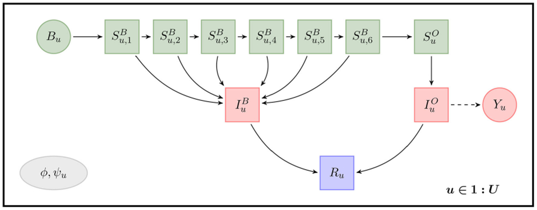
Flow diagram for the polio panel model. Each individual resides in exactly one of the compartments denoted by square boxes. Solid arrows represent possible transitions into a new compartment. Circles represent observed variables: the reported incidence, Yu, and births, Bu. The dependence of Yu on is denoted by a dashed arrow. Colors and rows representdisease status: unexposed isgreen (top row); infected is red (middle row); recovered is purple (bottom row). The panel structure is indicated by the replication of this model over u ∈ 1 : U. The shared parameter vector ϕ = (ρ, σdem, ψ, τ) and unit-specific parameter ψu = (bu,1:6, σenv,u, , ) are identified in the gray ellipse.
Since duration of infection is comparable to the one-month reporting aggregation, a discrete time model may be appropriate. The model is therefore specified only at times tu,n = tn = 1932 + (4 + n)/12 for n = 0, … , 249. We write
The mean force of infection, in units of yr−1, is modeled as
where Pu,n is a census population covariate for state u interpolated to time tn and seasonality of transmission is modeled as
with {ξk(t), k = 1, … , K} being a periodic B-spline basis. We set K = 6. The force of infection has a stochastic perturbation,
where ϵu,n is a Gamma random variable with mean 1 and variance . These two terms capture variation on the environmental and demographic scales, respectively (Bretó et al. 2009). All compartments suffer a mortality rate, set at δ = [60 yr]−1 for all states. Within each month, all susceptible individuals are modeled as having exposure to constant competing hazards of mortality and polio infection. The chance of remaining in the susceptible population when exposed to these hazards for one month is therefore
with the chance of polio infection being
We employ a continuous population model: writing Bu,n for births in month n for state u, the full set of model equations is,
The model for the reported observations, conditional on the latent process, is a discretized normal distribution truncated at zero, with both environmental and Poisson-scale contributions to the variance
where round(x) obtains the integer closest to x. Additional parameters are used to specify initial values for the latent process at time t0 = 1932 + 4/12. We will suppose there are parameters that specify the population in each compartment at time t0 via
The initial conditions are simplified by ignoring infant infections at time t0. Thus, we set and use monthly births in the preceding months (ignoring infant mortality) to fix for k = 1, … , 6. The estimated initial conditions for state u are then defined by the two parameters and , since the initial recovered population, Ru,0, is specified by subtraction of all the other compartments from the total initial population, Pu,0.
Figure 3 shows the profile likelihood for the shared reporting rate, ρ, evaluated across a wide interval to investigate large-scale features of the likelihood surface. Including a marginal maximization step in PIF leads to gains in agreement with the findings of Figure 1. Figure 3 indicates an MLE around 0.02 and so this parameter range was studied further in a higher resolution profile in Figure 4. On this localized plot, we can see Monte Carlo error of order 10 log units in the maximization and evaluation of the log-likelihood. Since construction of this plot employed 528.0 core days of computational effort, we had limited capacity for further reductions in Monte Carlo error by further increases in computation. Fortunately, MCAP methodology is able to handle Monte Carlo error on this scale: see, for example, the noisiest profile in Figure 1 using only joint maximization. The resulting 95% confidence interval from Figure 4 is (0.016, 0.020), which is consistent with estimates for the fraction of polio infections leading to acute paralysis in USA in this era (Melnick and Ledinko 1953). By contrast, Martinez-Bakker, King, and Rohani (2015) found point estimates ranging from 0.0025 to 0.03 when analyzing each state separately, with wide confidence intervals evident from the profiles in their Figures S9–S17.
Figure 3.
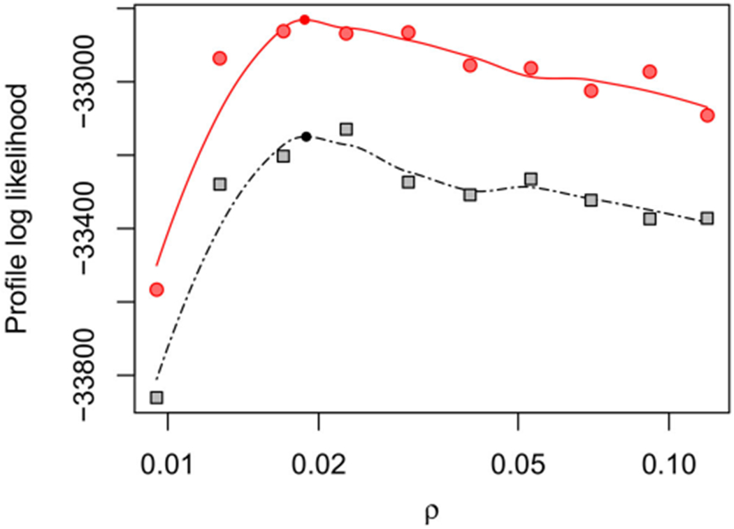
Profile log-likelihood of ρ for the polio model, computed with marginal maximization for unit-specific parameters (red circles and line) and without (black squares and line) with algorithmic parameters in Table S-1 in the supplement. Figure 4 gives a closer look in a neighborhood of the maximum and constructs a confidence interval.
Figure 4.
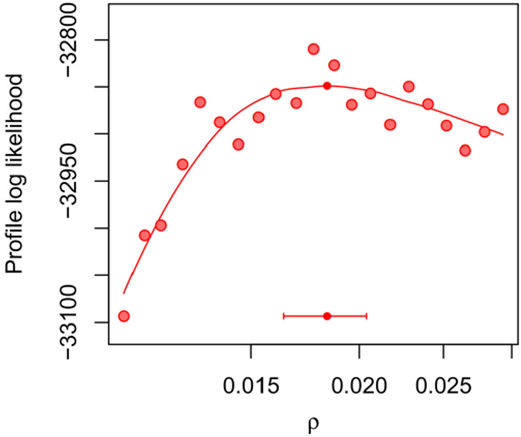
Profile log-likelihood of ρ for the polio model, computed in a neighborhood of the MLE. The horizontal bar shows a 95% MCAP confidence interval with a small filled circle marking the MLE obtained with algorithmic parameters in Table S-1 in the supplement.
Likelihood-based inference for data on this scale (U = 49, Nu = 249) has been considered intractable for general nonlinear PanelPOMP models using previous methodology. Indeed, even for a single observed time series, inference for general nonlinear POMP models has only recently become routine (King, Nguyen, and Ionides 2016). Evidently, the difficulties are a result of model complexity as much as the sheer volume of data. The interaction of model complexity with a modest increase in data size is the current challenge.
7. Dynamic Variation in Sexual Contact Rates
We demonstrate PIF for analysis of panel data on sexual contacts, using the model and data of Romero-Severson et al. (2015). The data consist of many short time series, a common situation in classical longitudinal analysis. We show that PIF provides useful flexibility to permit consideration of scientifically relevant dynamic models including latent dynamic variables.
Basic population-level disease transmission models suppose equal contact rates for all individuals in a population (Keeling and Rohani 2008). Sometimes these models are extended to permit heterogeneity between individuals. Heterogeneity within individuals over time has rarely been considered, yet, there have been some indications that dynamic behavioral change plays a substantial role in the HIV epidemic. Romero-Severson et al. (2015) quantified dynamic changes in sexual behavior by fitting a model for dynamic variation in sexual contact rates to panel data from a large cohort study of HIV-negative gay men (Vittinghoff et al. 1999). Here, weanalyzethedataon totalsexual contacts over Nu = 4 consecutive 6-month periods for the U = 882 men in the study who had no missing observations. A sample of the time series in this panel is plotted in the supplement.
For behavioral studies, we interpret “mechanistic model” broadly to mean a mathematical model describing phenomena of interest via interpretable parameters. In this context, we want a model that can describe (i) differences between individuals; (ii) differences within individuals over time; (iii) flexible relationships between mean and variance of contact rates. Romero-Severson et al. (2015) developed a PanelPOMP model capturing these phenomena. Suppose that each individual u ∈ 1 : U has a latent time-varying rate Λu(t) of making a sexual contact. Each data point, , is the number of reported contacts for individual u between time tu,n−1 and tu,n. Integrating the unobserved process {Λu(t)} gives the conditional expected value in (10) of contacts for individual u in reporting interval n, via
where α is an additional secular trend that accounts for the observed decline in reported contacts. A basic stochastic model for homogeneous count data would model as a Poisson random variable with mean and variance equal to Cu,n (Keeling and Rohani 2008). However, the variance in the data is much higher than the mean (Romero-Severson et al. 2012). Negative binomial processes provide a route to modeling dynamic overdispersion (Bretó and Ionides 2011). Here, we suppose that
| (10) |
a conditional negative binomial distribution with mean Cu,n and variance . Here, Du is called the dispersion parameter, with the Poisson model being recovered in the limit as Du becomes large. The dispersion, Du, can model increased variance compared to the Poisson distribution for individual contacts, but does not result in autocorrelation between measurements on an individual over time, which is observed in the data. To model this autocorrelation, we suppose that individual u has behavioral episodes of exponentially distributed duration within which {Λu(t)} is constant, but the individual enters new behavioral episodes at rate μR. At the start of each episode, {Λu(t)} takes a new value drawn from a Gamma distribution with mean μX and standard deviation σX. Therefore, at each time t,
To complete the model, we also assume Du ~ Gamma(μD, σD). The parameter vector is θ = (μX, σX, μD, σD, μR, α).
Figure 5 constructs a profile likelihood confidence interval for μR. This result is comparable to Web Figure 1 of Romero-Severson et al. (2015), however, here we have shown how this example fits into a general methodological framework. The profile demonstrates an intermediate level of computational challenge between the relatively simple Gompertz example of Section 5 and the extensive data, complex model, and correspondingly larger Monte Carlo computations of Section 6. Figure 5 took 68.7 core days to compute. No marginal maximization was necessary for this example, since all parameters were shared between all units.
Figure 5.
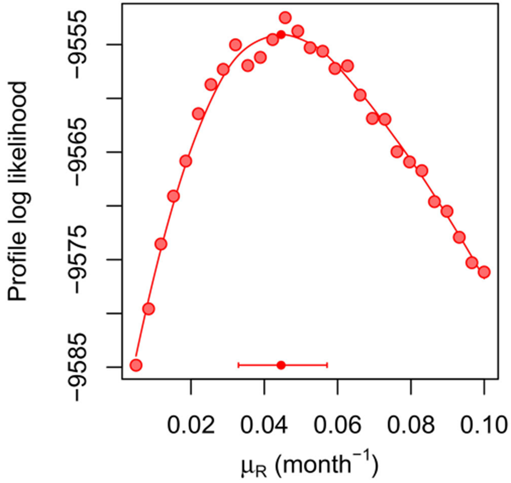
Profile log-likelihood of μR for a panel of size U = 882 for the contacts model. The horizontal bar shows a 95% MCAP confidence interval with a small filled circle marking the MLE obtained with algorithmic parameters in Table S-1 in the supplement.
8. Discussion
When panel data are short, relative to the complexity of the model under consideration, there may be little information in the data about each unit-specific parameter. In such cases, it can be appropriate to replace some unit-specific parameters by latent random variables. By analogy with linear regression analysis, these unit-specific latent random variables are called random effects, and unit-specific parameters treated as unknown constants are called fixed effects. Models with random effects are also called hierarchical models, since an additional hierarchy of modeling is required to describe the additional latent variables, and parameters of the random effect distribution are consequently termed hyperparameters. From the perspective of statistical inference, using random effects reduces the number of fitted parameters, at the expense of adding additional modeling assumptions. From the perspective of computation, random effects reduce the dimensionality of the likelihood optimization challenge, while increasing the dimensionality of the latent space which must be integrated over to evaluate the likelihood. The use of random effects provides an opportunity for the estimation of individual unit-specific effects to borrow strength from other panel units, via estimation of the hyperparameters. Therefore, random effects can have particular value if one is interested in estimating the unit-specific effects. However, when the research question is focused on shared parameters or higher-level model structure decisions such as whether a parameter should be included in the model, the individual unit-specific parameters can be a distraction. Rather than spending time developing and justifying a distribution for the random effects, simpler statistical reasoning can be obtained by avoiding these issues and employing fixed effects.
The sexual contact model has random effects Du and has no fixed effects. As discussed above, this is appropriate for panel data with very short time series. By contrast, the polio data are relatively long time series, enabling the use of fixed effects.
Panel time series analysis shares similarities with functional data analysis (Ramsay and Silverman 1997). Within functional data analysis, a representation of dynamic mechanisms can be incorporated via principal differential analysis (Ramsay 1996). Partially observed stochastic dynamic models are not within the usual scope of the field of functional data analysis, though there is no need for a hard line separating functional data analysis from panel data analysis.
We wrote an R package panelPomp (available at https://github.com/cbreto/panelPomp) that provides a software environment for developing methodology and data analysis tools for PanelPOMP models extending the pomp package (King, Nguyen, and Ionides 2016). The implementation of PIF in panelPomp was used for the results of this article. PIF and the panelPomp package have already proved useful for scientific investigations (Ranjeva et al. 2017, 2018).
Iterated filtering algorithms provide an approach to plug-and-play full-information likelihood-based inference that has been applied in challenging nonlinear mechanistic time series analyses, especially in epidemiology (reviewed by Bretó 2018). Reduced information methods, such as those using simulations to compare the data with a collection of summary statistics, can lead to substantial losses in statistical efficiency (Fasiolo, Pya, and Wood 2016; Shrestha, King, and Rohani 2011). Particle Markov chain Monte Carlo (Andrieu, Doucet, and Holenstein 2010) provides a route to plug-and-play full-information Bayesian inference, but the methodology requires computational feasibility of log-likelihood estimates with a standard error of around 1 log unit (Doucet et al. 2015). PIF is the first plug-and-play full-information likelihood-based approach demonstrated to be applicable on general partially observed nonlinear stochastic dynamic models for panel data analysis on the scale we have considered.
Supplementary Material
Acknowledgments
Funding
This research was supported by National Science Foundation grant DMS-1308919 and National Institutes of Health grants U54-GM111274, U01-GM110712, and R01-AI101155.
Footnotes
Color versions of one or more of the figures in the article can be found online at www.tandfonline.com/r/JASA.
Supplementary materials for this article are available online. Please go to www.tandfonline.com/r/JASA.
This article has been republished with minor changes. These changes do not impact the academic content of the article.
Supplement to “Panel data analysis via mechanistic models”: Supporting theoretical derivations, plots, and tables. (pdf)
Code: files to reproduce the main text (ms.Rnw) and supplement (supp.Rnw), as described in the README file. These files load R packages available from CRAN, as well as R packages bikpanel (for which we include the source code) and panelPomp (available from https://github.com/cbreto/panelPomp). (zip)
References
- Andrieu C, Doucet A, and Holenstein R (2010), “Particle Markov Chain Monte Carlo Methods,” Journal of the Royal Statistical Society, Series B, 72,269–342. [Google Scholar]
- Bartolucci F, Farcomeni A, andPennoni F (2012), Latent Markov Models for Longitudinal Data, Boca Raton, FL: CRC Press. [Google Scholar]
- Bengtsson T, Bickel P, and Li B (2008), “Curse-of-Dimensionality Revisited: Collapse of the Particle Filter in Very Large Scale Systems,” in Probability and Statistics: Essays in Honor of David A Freedman, eds. Speed T and Nolan D, Beachwood, OH: Institute of Mathematical Statistics, pp. 316–334. [Google Scholar]
- Bjørnstad ON, Finkenstädt BF, and Grenfell BT (2002), “Dynamics of Measles Epidemics: Estimating Scaling of Transmission Rates Using a Time Series SIR Model,” Ecological Monographs, 72, 169–184. [Google Scholar]
- Bjørnstad ON, and Grenfell BT (2001), “Noisy Clockwork: Time Series Analysis of Population Fluctuations in Animals,” Science, 293, 638–643. [DOI] [PubMed] [Google Scholar]
- Bossy M, Gobet E, and Talay D (2004), “A Symmetrized Euler Scheme for an Efficient Approximation of Reflected Diffusions,” Journal of Applied Probability, 41, 877–889. [Google Scholar]
- Bretó C (2018), “Modeling and Inference for Infectious Disease Dynamics: A Likelihood-Based Approach,” Statistical Science, 33, 57–69. [DOI] [PMC free article] [PubMed] [Google Scholar]
- Bretó C, He D, Ionides EL, and King AA (2009), “Time Series Analysis via Mechanistic Models,” Annals of Applied Statistics, 3, 319–348. [Google Scholar]
- Bretó C, and Ionides EL (2011), “Compound Markov Counting Processes and Their Applications to Modeling Infinitesimally Over-Dispersed Systems,” Stochastic Processes and Their Applications, 121,2571–2591. [Google Scholar]
- Cauchemez S, Carrat F, Viboud C, Valleron AJ, and Boelle PY (2004), “A Bayesian MCMC Approach to Study Transmission of Influenza: Application to Household Longitudinal Data,” Statistics in Medicine, 23, 3469–3487. [DOI] [PubMed] [Google Scholar]
- Chen Y, Shen K, Shan S-O, and Kou S (2016), “Analyzing SingleMolecule Protein Transportation Experiments via Hierarchical Hidden Markov Models,” Journal of the American Statistical Association, 111,951–966. [DOI] [PMC free article] [PubMed] [Google Scholar]
- Dai L, and Schön TB (2016), “Using Convolution to Estimate the Score Function for Intractable State-Transition Models,” IEEE Signal Processing Letters, 23, 498–501. [Google Scholar]
- Del Moral P (2004), Feynman-Kac Formulae: Genealogical and Interacting Particle Systems With Applications, New York: Springer. [Google Scholar]
- Del Moral P, and Guionnet A (2001), “On the Stability of Interacting Processes With Applications to Filtering and Genetic Algorithms,” Annales de l’Institut Henri Poincaré (B) Probability and Statistics, 37,155–194. [Google Scholar]
- Dobson A (2014), “Mathematical Models for Emerging Disease,” Science, 346, 1294–1295. [DOI] [PubMed] [Google Scholar]
- Donnet S, and Samson A (2013), “A Review on Estimation of Stochastic Differential Equations for Pharmacokinetic/Pharmacodynamic Models,” Advanced Drug Delivery Reviews, 65, 929–939. [DOI] [PubMed] [Google Scholar]
- Douc R, Moulines E, and Stoffer D (2014), Nonlinear Time Series: Theory, Methods and Applications With R Examples, BocaRaton, FL: CRC Press. [Google Scholar]
- Doucet A, Jacob PE, and Rubenthaler S (2015), “Derivative-Free Estimation of the Score Vector and Observed Information Matrix With Application to State-Space Models,” arXiv no. 1304.5768v3. [Google Scholar]
- Doucet A, Pitt MK, Deligiannidis G, and Kohn R (2015), “Efficient Implementation of Markov Chain Monte Carlo When Using an Unbiased Likelihood Estimator,” Biometrika, 102,295–313. [Google Scholar]
- Fasiolo M, Pya N, and Wood SN (2016), “A Comparison of Inferential Methods for Highly Nonlinear State Space Models in Ecology and Epidemiology,” Statistical Science, 31, 96–118. [Google Scholar]
- He D, Ionides EL, and King AA (2010), “Plug-and-Play Inference for Disease Dynamics: Measles in Large and Small Towns as a Case Study,” Journal of the Royal Society Interface, 7, 271–283. [DOI] [PMC free article] [PubMed] [Google Scholar]
- Heiss F (2008), “Sequential Numerical Integration in Nonlinear State Space Models for Microeconometric Panel Data,” Journal of Applied Econometrics, 23, 373–389. [Google Scholar]
- Hsiao C (2014), Analysis of Panel Data, Cambridge, UK: Cambridge University Press. [Google Scholar]
- Ionides EL, Bhadra A, Atchadé Y, and King AA (2011), “Iterated Filtering,” Annals of Statistics, 39, 1776–1802. [Google Scholar]
- Ionides EL, Bretó C, and King AA (2006), “Inference for Nonlinear Dynamical Systems,” Proceedings of the National Academy of Sciences of the United States of America, 103, 18438–18443. [DOI] [PMC free article] [PubMed] [Google Scholar]
- Ionides EL, Bretó C, Park J, Smith RA, and King AA (2017), “Monte Carlo Profile Confidence Intervals for Dynamic Systems,” Journal of the Royal Society Interface, 14, 1–10. [DOI] [PMC free article] [PubMed] [Google Scholar]
- Ionides EL, Nguyen D, Atchadé Y, Stoev S, and King AA (2015), “Inference for Dynamic and Latent Variable Models via Iterated, Perturbed Bayes Maps,” Proceedings of the National Academy of Sciences of the United States of America, 112, 719–724. [DOI] [PMC free article] [PubMed] [Google Scholar]
- Keeling MJ, and Rohani P (2008), Modeling Infectious Diseases in Humans and Animals, Princeton, NJ: Princeton University Press. [Google Scholar]
- King AA, Nguyen D, and Ionides EL (2016), “Statistical Inference for Partially Observed Markov Processes via the R Package Pomp,” Journal of Statistical Software, 69, 1–43. [Google Scholar]
- Le Gland F, and Oudjane N (2004), “Stability and Uniform Approximation of Nonlinear Filters Using the Hilbert Metric and Application to Particle Filters,” The Annals of Applied Probability, 14, 144–187. [Google Scholar]
- Martinez-Bakker M, Bakker KM, King AA, and Rohani P (2014), “Human Birth Seasonality: Latitudinal Gradient and Interplay With Childhood Disease Dynamics,” Proceedings of the Royal Society of London B: Biological Sciences, 281, 20132438. [DOI] [PMC free article] [PubMed] [Google Scholar]
- Martinez-Bakker M, King AA, and Rohani P (2015), “Unraveling the Transmission Ecology of Polio,” PLoS Biology, 13,e1002172. [DOI] [PMC free article] [PubMed] [Google Scholar]
- Melnick JL, and Ledinko N (1953), “Development of Neutralizing Antibodies Against the Three Types of Poliomyelitis Virus During an Epidemic Period. The Ratio of Inapparent Infection to Clinical Poliomyelitis,” American Journal ofHygiene, 58, 207–222. [DOI] [PubMed] [Google Scholar]
- Mesters G, and Koopman SJ (2014), “Generalized Dynamic Panel Data Models With Random Effects for Cross-Section and Time,” Journal of Econometrics, 180, 127–140. [Google Scholar]
- Patel M, and Orenstein W (2016), “A World Free of Polio—The Final Steps,” New England Journal of Medicine, 374, 501–503. [DOI] [PubMed] [Google Scholar]
- Pons-Salort M, and Grassly NC (2018), “Serotype-Specific Immunity Explains the Incidence of Diseases Caused by Human Enteroviruses,” Science, 361, 800–803. [DOI] [PMC free article] [PubMed] [Google Scholar]
- Ramsay JO (1996), “Principal Differential Analysis: Data Reduction by Differential Operators,” Journal of the Royal Statistical Society, Series B, 58, 495–508. [Google Scholar]
- Ramsay JO, and Silverman BW (1997), Functional Data Analysis, New York: Springer-Verlag. [Google Scholar]
- Ranjeva SL, Baskerville EB, Dukic V, Villa LL, Lazcano-Ponce E, Giuliano AR, Dwyer G, and Cobey S (2017), “Recurring Infection With Ecologically Distinct HPV Types Can Explain High Prevalence and Diversity,” Proceedings of the National Academy of Sciences of the United States of America, 114, 13573–13578. [DOI] [PMC free article] [PubMed] [Google Scholar]
- Ranjeva S, Subramanian R, Fang VJ, Leung GM, Ip DK, Perera RA, Peiris JSM, Cowling BJ, and Cobey S (2018), “Age-Specific Differences in the Dynamics of Protective Immunity to Influenza,” bioRxiv no. 330720. [DOI] [PMC free article] [PubMed] [Google Scholar]
- Romero-Severson EO, Alam SJ, Volz EM, and Koopman JS (2012), “Heterogeneity in Number and Type of Sexual Contacts in a Gay Urban Cohort,” Statistical Communications in Infectious Diseases, 4. [DOI] [PMC free article] [PubMed] [Google Scholar]
- Romero-Severson E, Volz E, Koopman J, Leitner T, and Ionides E (2015), “Dynamic Variation in Sexual Contact Rates in a Cohort of HIV - Negative Gay Men,” American Journal of Epidemiology, 182, 255–262. [DOI] [PMC free article] [PubMed] [Google Scholar]
- Shrestha S, King AA, and Rohani P (2011), “Statistical Inference for Multi-Pathogen Systems,” PLoS Computational Biology, 7, e1002135. [DOI] [PMC free article] [PubMed] [Google Scholar]
- Smith RA, Ionides EL, and King AA (2017), “Infectious Disease Dynamics Inferred From Genetic Data via Sequential Monte Carlo,” Molecular Biology and Evolution, 34, 2065–2084. [DOI] [PMC free article] [PubMed] [Google Scholar]
- Vittinghoff E, Douglas J, Judon F, McKiman D, MacQueen K, and Buchinder SP (1999), “Per-Contact Risk of Human Immunodeficiency Virus Transmission Between Male Sexual Partners,” American Journal of Epidemiology, 150,306–311. [DOI] [PubMed] [Google Scholar]
- Wickham H (2014), “Tidy Data,” Journal of Statistical Software, 59, 1–23.26917999 [Google Scholar]
- Winsor CP (1932), “The Gompertz Curve as a Growth Curve,” Proceedings of the National Academy of Sciences of the United States of America, 18, 1–8. [DOI] [PMC free article] [PubMed] [Google Scholar]
- Wood SN (2010), “Statistical Inference for Noisy Nonlinear Ecological Dynamic Systems,” Nature, 466, 1102–1104. [DOI] [PubMed] [Google Scholar]
- Yang Y, Halloran ME, Daniels MJ, Longini IM, Burke DS, and Cummings DAT (2010), “Modeling Competing Infectious Pathogens From a Bayesian Perspective: Application to Influenza Studies With Incomplete Laboratory Results,” Journal of the American Statistical Association, 105, 1310–1322. [DOI] [PMC free article] [PubMed] [Google Scholar]
- Yang Y, Longini IM Jr., Halloran ME, and Obenchain V (2012), “A Hybrid EM and Monte Carlo EM Algorithm and Its Application to Analysis of Transmission of Infectious Diseases,” Biometrics, 68, 1238–1249. [DOI] [PMC free article] [PubMed] [Google Scholar]
Associated Data
This section collects any data citations, data availability statements, or supplementary materials included in this article.