Multinomial and ordinal Logistic regression analyses with multi-categorical variables using R

It is essential in a standard linear regression analysis that dependent variables are continuous. However, using the standard linear regression for the analysis of a double-level or multi-level outcome can lead to unsatisfactory results because the validity of this regression model relies on the variability of the outcome being the same for all values of predictors, which is contrary to the nature of double-level or multi-level outcomes (1). Therefore, when the dependent variable consists of several categories, a maximum likelihood estimator, such as multinomial logit or probit, should be used instead of the ordinary least square estimator (2). Logistic regression can be used to describe the relationship between an independent variable(s) (either continuous or not) and a dichotomous or multi-categorical dependent variable as a supplementary variable to the standard linear regression.

Zhou et al. (3) elaborated a series of reliable methodologies using the R software to construct clinical prediction models with detailed steps and operable code examples, according to different types of clinical data and categories of variables. They summarized the process of the construction of practical clinical prediction models (nomograms), including data screening, primary model training, and internal and external validations, which was an extraordinary work and a practical reference in the field of statistics (4-6). Based on this study, a simpler and more accurate prediction model was introduced as an extension by Bi et al. (7), which was designed for extracting polynomial equations and calculating the points of each variable together with survival probabilities.

The general objective of logistic regression models is to predict outcomes using variables based on certain existing data, which have been applied in medical research for various diseases (8). In the study by Zhou and his colleagues (3), the authors converted multi-categorical outcomes into dichotomous ones and introduced a dichotomous logistic regression using R codes. However, multi-categorical outcomes can be directly applied in multinomial or ordinal logistic regression analyses in the R software, although the results might be difficult to be interpreted with more complicated steps. This study aimed to display the methods and processes used to apply multi-categorical variables in logistic regression models in the R software environment.

The sample data was made up of patients registered in the SEER database in 2015 with diagnoses of lung adenocarcinomas. Patients with unclear race, primary site(s) of their tumors, differentiation grade of their tumors, tumor stage (AJCC, 6^th edition), or cause of their death were excluded. Finally, 6,483 patients met the inclusion and exclusion criteria, of which 3,000 were randomly selected for the following analysis. Age, sex, race, primary site of the tumor, cell differentiation grade, AJCC stage of the tumor, and history of chemotherapy, were chosen as independent variables. The ages of included patients, ranging from 20 to 100 years, were divided into eight groups, labeled as “AgeGroup”. Also, several subgroup variables were defined for each of the other six variables: “Sex” (male and female), “Race” (white, black, and others), “PrimarySite” (main, upper lobe, middle lobe, lower lobe, and overlapped), “Grade” (I–IV), “Stage” (I–IV), and “Chemotherapy” (yes and no or unknown). Survival status labeled as “Causespecificdeathclassification” was defined as the dependent variable consisting of three categories: alive, dead due to lung cancer, and dead due to other causes. Survival months were extracted for constructing an ordinal outcome. Using the dplyr package in R, the survival months were converted into “SurvivalStatus” based on the tertiles of survival months. Patient outcomes were defined as “0 = no response” for those whose survival months are in the first third tertile; “1 = partial response” and “2 = complete response” were defined as outcomes for patients whose survival months are in the middle and last third tertiles, respectively.

Multinomial logistic regressions can be applied for multi-categorical outcomes, whereas ordinal variables should be preferentially analyzed using an ordinal logistic regression model. Besides, if the ordinal model does not meet the parallel regression assumption, the multinomial one will still be an alternative (9). A multinomial regression analysis was started as follows with four main steps.

Multinomial regression analysis

Step 1: data preparation

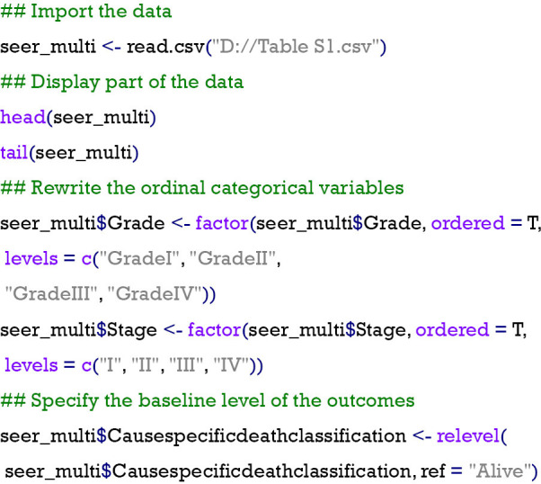
First, the sample data set was imported into R, and the ordinal categorical variables (“Grade” and “Stage”) in the data were rewritten as ordered factors using the factor function. The level of the outcome to be used as the baseline was selected and specified using the relevel function. Here, “Alive” was defined as a baseline to be compared with “Dead (attributable to this cancer dx)” and “Dead of other cause” in the regression. The codes in R are shown below. The data we used in the analyses can be found in http://cdn.amegroups.cn/static/application/949e8411be91d730d1670c07b0d01072/10.21037atm-2020-57-1.pdf.

Step 2: model running

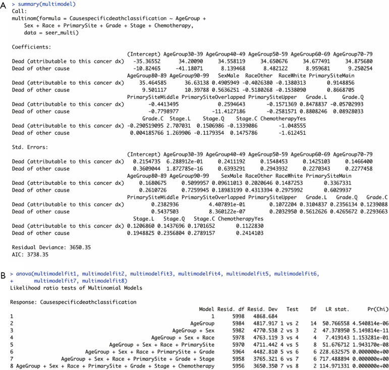
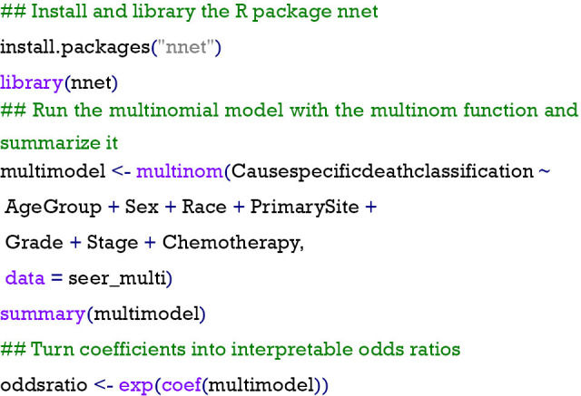
Second, the model was run using the multinorm function in the nnet package in R as follows. In the outputs of the summary of the model (Figure 1A), a block of coefficients displayed as logged odds was shown followed by their standard errors.

Figure 1.

Outputs of the multinomial logistic regression model. (A) Summary of the model. (B) Results of ANOVA. Grade. L: Grade II; Grade. Q: Grade III; Grade. C: Grade IV; Stage. L: Stage II; Stage. Q: Stage III; Stage. C: Stage IV.

Each of these blocks had one row of values corresponding to a model equation. In the first row, for instance, coefficients (logged odds) of each independent variable comparing “Dead (attributable to this cancer dx)” with “Alive” were shown. The coefficients were pulled out from the model and converted into interpretable odds ratios additionally by exponential analyses using the exp() command.

Step 3: tests of the coefficients

After constructing the regression model, the next thing was to calculate P values of the regression coefficients using Wald tests (z tests used in this study). R codes and part of the outputs are shown below. The coefficients were considered to be of significance with a two-tailed value of P<0.05, and no significance was attributed otherwise. Focusing on the block of P values below, variables with significant P values of their coefficients were determined as significant prognostic factors that contributed significantly differently to cancer-specific death or death of other causes rather than to survival in patients with lung adenocarcinoma.

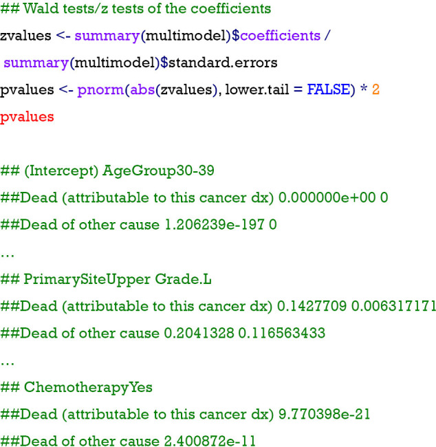
Combining the results of the logged odds (coefficients) in Figure 1A with those of the P values in this part, the coefficients could be interpreted as changes in odds for a certain category comparing with another category in each independent variable. For example, the logged odds of cancer-specific death due to lung adenocarcinoma versus survival significantly increased by approximately 0.848 if moving from differentiation “Grade I” to “Grade II” of tumors with the logged odds being 8.478837e-1 and the P value being 6.317171e-3.

Step 4: tests and validations of the model

Last but not least, the analysis of variance (ANOVA) was used to test the significance of this regression model using the ANOVA function. Using this function, the goodness of fit of the model was assessed indirectly by comparing regression models with the regression models before adding variables. Here, significance was considered with a relaxed value of P<0.10 or P<0.15 when comparing multiple regression models. The results are shown in Figure 1B. The P value in the last row (model 1 vs. model 8) indicated that the proposed multinomial regression model was of significance. Besides, the second to the eighth models were all significant improvements over previous models because their P values were generally less than 0.15.

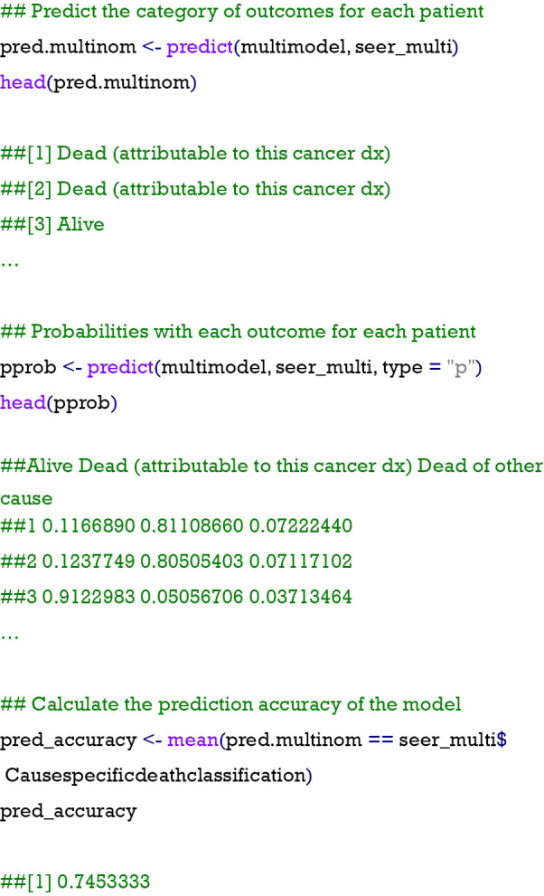
Additionally, the regression model was further validated by predicting the survival outcomes of each patient in the data set together with the probabilities of each outcome using the predict function in R as follows. The prediction accuracy of the model was obtained by calculating the mean of predicted probabilities of the original survival outcomes of each patient. The results demonstrated that 74.5% of the clinical survival outcomes of the patients in the present data set were verified to be correct using the regression model, indicating that this multinomial regression model had strong reliability.

Ordinal logistic regression model

Next, an ordinal logistic regression was displayed similarly using the R software with the sample data. Here, five steps in total should be taken in constructing an ordinal logistic regression model as follows.

Step 1: data preparation

This step was basically the same as the processes in the first step of multinomial regression analysis, including data import and variable redefinition. Relevant R codes can refer to the previous section of multinomial regression.

Step 2: model running

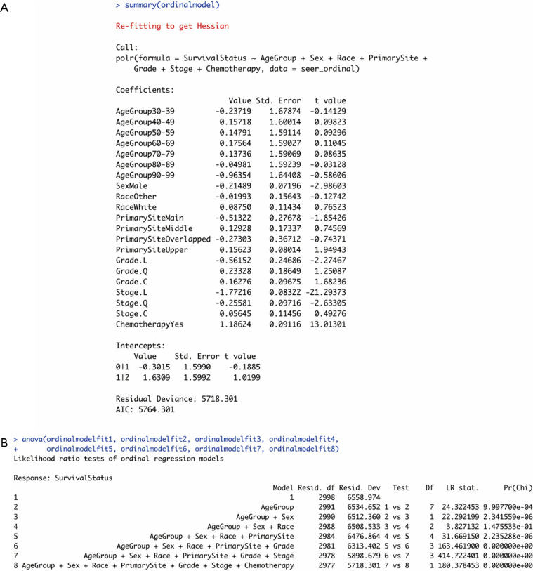
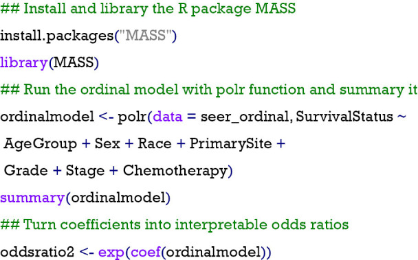
The ordinal regression model was run using the polr function in the MASS package of R. The codes are shown as follows. The summary of the model (Figure 2A) also contained a block of coefficients displayed as logged odds, followed by their standard errors together with t values. These coefficients could also be converted into interpretable odds ratios using the exp() command.

Figure 2.

Outputs of the ordinal logistic regression model. (A) Summary of the model. (B) Results of ANOVA. Grade. L: Grade II; Grade. Q: Grade III; Grade. C: Grade IV; Stage. L: Stage II; Stage. Q: Stage III; Stage. C: Stage IV.

Each row of values corresponded to a model equation with a category of a certain independent variable. The coefficients in each row were indicators of the logged times the patient survival will increase by one degree (“0 = no response” to “1 = partial response” or “1 = partial response” to “2 = complete response”) when one of their clinicopathological characteristics changes from the reference category to a certain category displayed in the beginning of the row.

Step 3: test of parallel lines

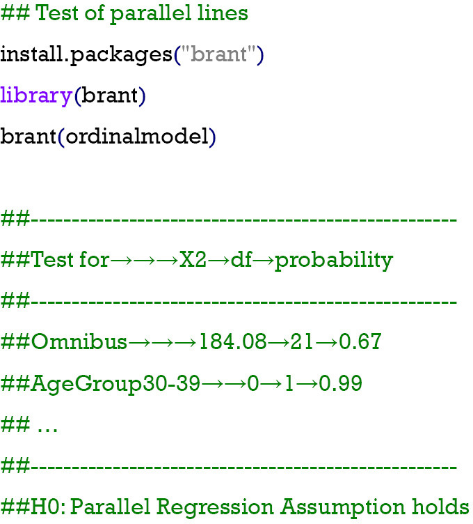
Parallel regression assumption or the proportional odds assumption is a necessity for the application of the ordinal logistic regression model for an ordered categorical variable; otherwise, the multinomial model described earlier has to be used. This assumption can be tested using a Brant test in the R software, which is available in the Brant package with the brant function. A P value higher than 0.05 may lead to the failure of rejecting the null hypothesis that the parallel regression assumption holds or that the coefficients do not differ across different cut points in the outcome variable. According to the codes and outputs, there was a P value of 0.67 in the “Omnibus” check, indicating the lack of evidence showing that the previous assumption has not been met. Therefore, the ordinal regression method was appropriate for the sample data set.

Step 4: test of the coefficients

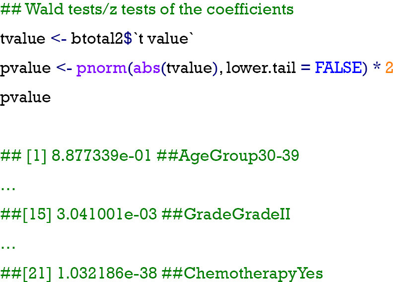
Different from the multinomial regression model, the ordinal regression model has provided the t values of each of the categories of variables that can be directly used to calculate the P values of the coefficients by Wald tests using the following codes. Combining the results of logged odds (coefficients) and their P values, the coefficients can be interpreted as changes in odds for a certain category of variables, but the interpretation is slightly different from the previous multinomial logistic regression. For example, if moving from differentiation “Grade I” to “Grade II” of tumors, the logged odds of the probability of patients being in the next degree of survival time (from “0 = no response” to “1 = partial response” or from “1 = partial response” to “2 = complete response”) will be decreased by −0.562 with significance.

Step 5: test and validations of the model

Same as the fourth step in multinomial regression, the significance of the ordinal regression model and the goodness of fit of the proposed model needs to be assessed using the ANOVA function. R codes can refer to the multinomial regression analysis section. Results (Figure 2B) indicated that the proposed ordinal regression model was significant, and the second to eighth models were validated to be significant improvements over each of their previous ones.

As in a multinomial regression model, further validations can be performed using the predict function. R codes can be found in the same step of the previous section. Here, our proposed multinomial regression model had relatively strong reliability since the accuracy was shown to be 52.2%.

Conclusions

In summary, two logistic regression methods were introduced in this study using the R software for multi-categorical variables in four basic steps of statistical regression: data preparation, model establishment, tests of the coefficients and the model, and model validations. The authors are grateful to Dr. Zhou and his colleagues for their contributions, which served as a valuable reference.

Supplementary

The article’s supplementary files as

Ethical statement: The authors are accountable for all aspects of the work in ensuring that questions related to the accuracy or integrity of any part of the work are appropriately investigated and resolved. Ethics approval has been exempted by the Ethics Committee of Zhongshan Hospital of Fudan University (Shanghai, China), as the SEER is a publicly available database, and data extracted from SEER are identified as nonhuman study.

References

- 1.LaValley MP. Logistic regression. Circulation 2008;117:2395-9. 10.1161/CIRCULATIONAHA.106.682658 [DOI] [PubMed] [Google Scholar]
- 2.Kwak C, Clayton-Matthews A. Multinomial logistic regression. Nurs Res 2002;51:404-10. 10.1097/00006199-200211000-00009 [DOI] [PubMed] [Google Scholar]
- 3.Zhou ZR, Wang WW, Li Y, et al. In-depth mining of clinical data: the construction of clinical prediction model with R. Ann Transl Med 2019;7:796. 10.21037/atm.2019.08.63 [DOI] [PMC free article] [PubMed] [Google Scholar]
- 4.Steyerberg EW, Vergouwe Y. Towards better clinical prediction models: seven steps for development and an ABCD for validation. Eur Heart J 2014;35:1925-31. 10.1093/eurheartj/ehu207 [DOI] [PMC free article] [PubMed] [Google Scholar]
- 5.Han K, Song K, Choi BW. How to Develop, Validate, and Compare Clinical prediction models involving radiological parameters: study design and statistical methods. Korean J Radiol 2016;17:339-50. 10.3348/kjr.2016.17.3.339 [DOI] [PMC free article] [PubMed] [Google Scholar]
- 6.Woodward M, Tunstall-Pedoe H, Peters SA. Graphics and statistics for cardiology: clinical prediction rules. Heart 2017;103:538-45. 10.1136/heartjnl-2016-310210 [DOI] [PMC free article] [PubMed] [Google Scholar]
- 7.Bi G, Li R, Liang J, et al. A nomogram with enhanced function facilitated by nomogramEx and nomogramFormula. Ann Transl Med 2020;8:78. 10.21037/atm.2020.01.71 [DOI] [PMC free article] [PubMed] [Google Scholar]
- 8.Tolles J, Meurer WJ. Logistic regression: Relating patient characteristics to outcomes. JAMA 2016;316:533-4. 10.1001/jama.2016.7653 [DOI] [PubMed] [Google Scholar]
- 9.García-Pérez MA. Statistical criteria for parallel tests: a comparison of accuracy and power. Behav Res Methods 2013;45:999-1010. 10.3758/s13428-013-0328-z [DOI] [PubMed] [Google Scholar]
Associated Data
This section collects any data citations, data availability statements, or supplementary materials included in this article.
Supplementary Materials