A distributional code for value in dopamine-based reinforcement learning

Abstract

Since its introduction, the reward prediction error (RPE) theory of dopamine has explained a wealth of empirical phenomena, providing a unifying framework for understanding the representation of reward and value in the brain^1–3. According to the now canonical theory, reward predictions are represented as a single scalar quantity, which supports learning about the expectation, or mean, of stochastic outcomes. In the present work, we propose a novel account of dopamine-based reinforcement learning. Inspired by recent artificial intelligence research on distributional reinforcement learning^4–6, we hypothesized that the brain represents possible future rewards not as a single mean, but instead as a probability distribution, effectively representing multiple future outcomes simultaneously and in parallel. This idea leads immediately to a set of empirical predictions, which we tested using single-unit recordings from mouse ventral tegmental area. Our findings provide strong evidence for a neural realization of distributional reinforcement learning.

The RPE theory of dopamine derives from work in the artificial intelligence (AI) field of reinforcement learning (RL)⁷. Since the link to neuroscience was first made, however, RL has made substantial advances^8,9, revealing factors that radically enhance the effectiveness of RL algorithms¹⁰. In some cases, the relevant mechanisms invite comparison with neural function, suggesting new hypotheses concerning reward-based learning in the brain^11–13. Here, we examine one particularly promising recent development in AI research and investigate its potential neural correlates. Specifically, we consider a computational framework referred to as distributional reinforcement learning (Figure 1a,b)^4–6.

Figure 1: Distributional value coding arises from a diversity of relative scaling of positive and negative prediction errors.

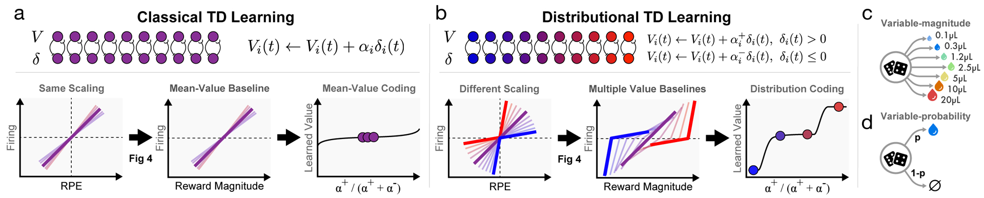
a, In the standard temporal difference (TD) theory of the dopamine system, all value predictors learn the same value V. Each dopamine cell is assumed to have the same relative scaling for positive and negative RPEs (left). This causes each value prediction (or value baseline) to be the mean of the outcome distribution (middle). Dotted lines indicate zero RPE or pre-stimulus firing. b, In our proposed model, distributional TD, different channels have different relative scaling for positive (α⁺) and negative (α⁻) RPEs. Red shading indicates α⁺ > α⁻, and blue shading indicates α⁻> α⁺. An imbalance between α⁺ and α⁻ causes each channel to learn a different value prediction. This set of value predictions collectively represents the distribution over possible rewards. c, We analyze data from two tasks. In the variable-magnitude task, there is a single cue, followed by a reward of unpredictable magnitude. d, In the variable-probability task, there are three cues, which each signal a different probability of reward, and the reward magnitude is fixed.

Like the traditional form of temporal difference RL, on which the dopamine theory was based, distributional RL assumes that reward-based learning is driven by a RPE, which signals the difference between received and anticipated reward^†. The key difference in distributional RL lies in the way that ‘anticipated reward’ is defined. In traditional RL, the reward prediction is represented as a single quantity: the average over all potential reward outcomes, weighted by their respective probabilities. Distributional RL, in contrast, employs a multiplicity of predictions. These predictions vary in their degree of optimism about upcoming reward. More optimistic predictions anticipate obtaining greater future rewards; less optimistic predictions anticipate more meager outcomes. Together, the entire range of predictions captures the full probability distribution over future rewards (more details in Supplement section 1.1).

Compared with traditional RL procedures, distributional RL can increase performance in deep learning systems by a factor of two or more^5,14,15, an effect that stems in part from an enhancement of representation learning (see Extended Data Figure 2, 3 and Supplement section 1.2). This suggests the intriguing question of whether RL in the brain might leverage the benefits of distributional coding. This question is encouraged both by the fact that the brain employs distributional codes in numerous other domains¹⁶, and that the mechanism of distributional RL is biologically plausible^6,17. Here we tested several surprising predictions of distributional RL using single unit recordings in the ventral tegmental area (VTA) of mice performing tasks with probabilistic rewards.

Different dopamine neurons utilize different value predictions.

In contrast to classical TD learning, distributional RL posits a diverse set of RPE channels, each of which carries a different value^‡ prediction, with varying degrees of optimism across channels. These value predictions in turn provide the reference points for different RPE signals, causing the latter also to differ in terms of optimism. As a startling consequence, a single reward outcome can simultaneously elicit positive RPEs (within relatively pessimistic channels) and negative RPEs (within more optimistic ones).

This translates immediately into a neuroscientific prediction, which is that dopamine neurons should display such diversity in ‘optimism.’ Suppose an agent has learned that a cue predicts a reward whose magnitude will be drawn from a probability distribution. In the standard RL theory, receiving a reward with magnitude below the mean of this distribution will elicit a negative RPE, while larger magnitudes will elicit positive RPEs. The reversal point – the magnitude where prediction errors transition from negative to positive – in standard RL is the expectation of the magnitude’s distribution. By contrast, in distributional RL, the reversal point differs across dopamine neurons according to their degree of optimism.

We tested for such reversal-point diversity in optogenetically verified dopaminergic VTA neurons, focusing on responses to receipt of liquid rewards, the volume of which was drawn at random on each trial from seven possible values (Figure 1c). As anticipated by distributional RL, but not by the standard theory, we found that dopamine neurons had substantially different reversal points, ranging from cells that reversed between the smallest two rewards to cells that reversed between the largest two rewards (Figure 2a,b). This diversity was not due to noise, as the reversal point estimated on a random half of the data was a robust predictor of the reversal point estimated on the other half of the data (R = 0.58, p = 1.8 × 10⁻⁵; Figure 2c). In fact, in response to the 5 μL reward, 13/40 cells had significantly above-baseline responses and 10/40 cells had significantly below-baseline responses. Note that while some cells appeared pessimistic and others optimistic, there was also a population of cells with approximately ‘neutral’ responses, as predicted by the distributional RL model (cf. Figure 2a, right panel).

Figure 2: Different dopamine neurons consistently reverse from positive to negative responses at different reward magnitudes.

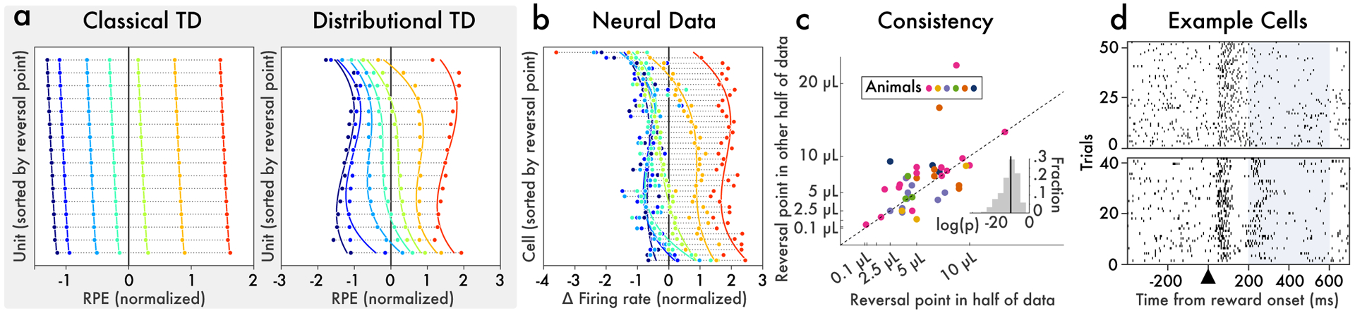
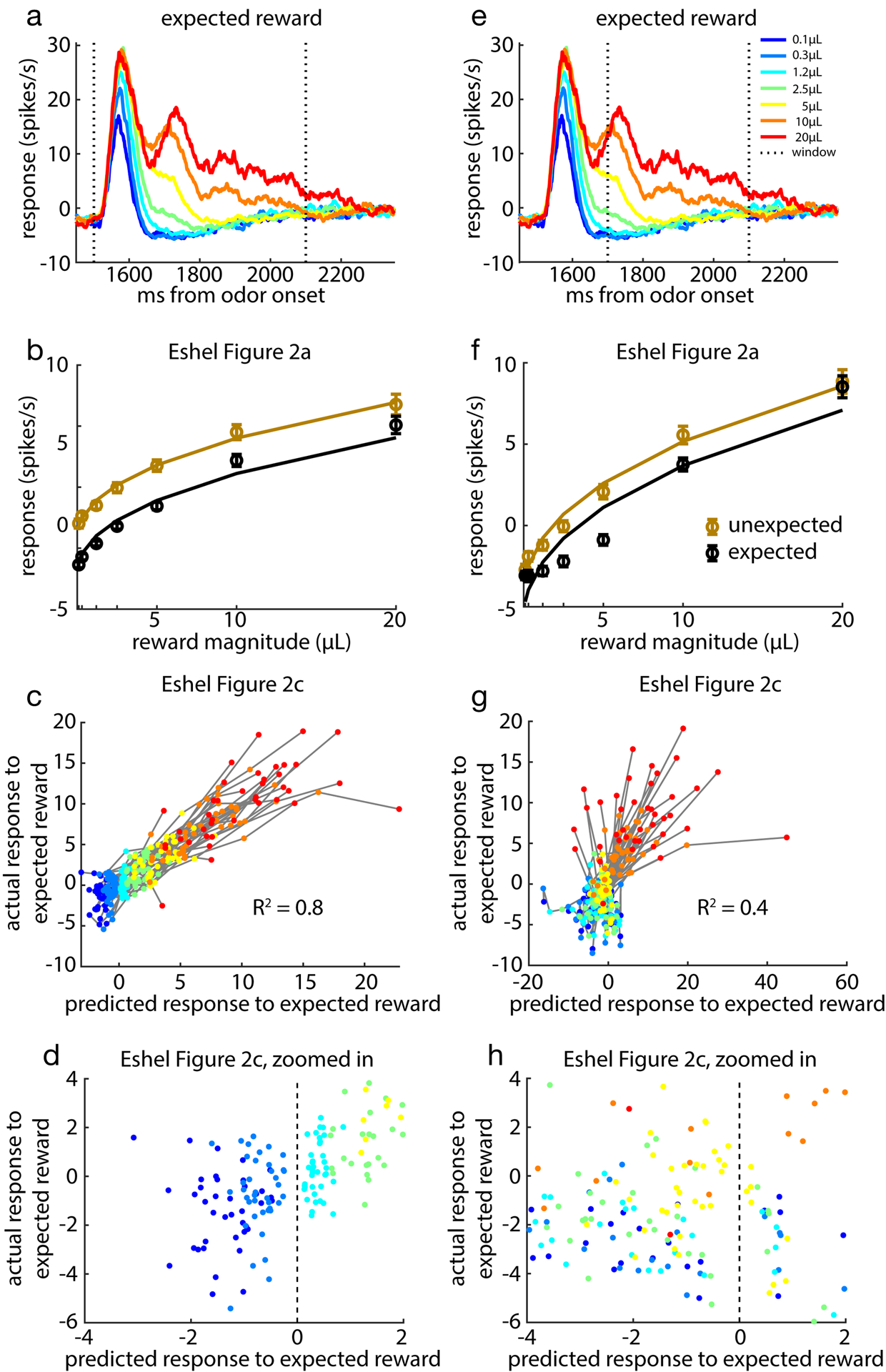
Variable-magnitude task from Eshel et al.³⁴. On each trial, the animal experiences one of seven possible reward magnitudes (0.1, 0.3, 1.2, 2.5, 5, 10, or 20 μL), selected randomly. a, RPEs produced by classical and distributional TD simulations. Each horizontal bar is one simulated neuron. Each dot color corresponds to a particular reward magnitude. The x-axis is the cell’s response (change in firing rate) when reward is delivered. Cells are sorted by reversal point. In classic TD, all cells carried approximately the same RPE signal. Note that the slight differences between cells arose from Gaussian noise added to the simulation; the differences between cells in the classic TD simulation were not statistically reliable. Conversely, in distributional TD, cells had reliably different degrees of optimism. Some responded positively to almost all rewards, and others responded positively to only the very largest reward. b, Responses recorded from light-identified dopamine neurons in behaving mice. Neurons differed markedly in their reversal points. c, To assess whether this diversity was reliable, we randomly partitioned the data into two halves and estimated reversal points independently in each half. We found that the reversal point estimated in one half was highly correlated with that estimated in the other half. d, Spike rasters for two example dopamine neurons from the same animal, showing responses to all trials when the 5 μL reward was delivered. We analyzed data from 200 to 600 ms after reward onset (highlighted), to exclude the initial transient which was positive for all magnitudes. During this epoch, the cell on the bottom fires above its baseline rate, while the cell on the top pauses.

A stronger test of our theory is whether this diversity also exists within a single animal. Most animals had too few cells for analysis, but within the single animal with the most cells recorded, reversal points estimated on half of the data were robustly predictive of reversal points estimated on the other half (p = 0.008). And in response to a single reward magnitude (5 μL), 6/16 cells had significantly above-baseline responses and 5/16 cells had significantly below-baseline responses. Finally, Figure 2d shows rasters of two example cells from this animal, exhibiting consistently opposite responses to the same reward.

Because the diversity we observe is reliable across trials, it cannot be explained by adding measurement noise to non-distributional TD models. As detailed in section 2 of the Supplement (also see Extended Data Figure 4), we also analyzed several more elaborate alternative models, and while some of these can give rise to the appearance of reversal-point diversity under some analysis methods, the same models are frankly contradicted by further aspects of the experimental data, which we report below.

While our first prediction dealt with the relationship between dopaminergic signaling and reward magnitude, dopaminergic RPE signals also scale with reward probability^2,18, and distributional RL leads to a prediction in this domain as well. Pursuing this, we analyzed data from a second task in which sensory cues indicated the probability of an upcoming liquid reward (Figure 1d). One cue indicated a 10% probability of reward, a different cue indicated a 50% probability, and a third a 90% probability. The standard RPE theory predicts that, considering responses at the time the cue is presented, all dopamine neurons should have the same relative spacing between 10%, 50% and 90% cue responses.^§

Distributional RL predicts, instead, that dopamine neurons should vary in their responses to the 50% cue: Some neurons should respond optimistically, emitting a RPE nearly as large as to the 90% cue. Others should respond pessimistically, emitting a RPE closer to the 10% cue response (Figure 3a). Labelling these two cases as optimistically and pessimistically biased, distributional RL predicts that dopamine neurons, as a population, should show concurrent optimistic and pessimistic coding for reward probability.

Figure 3: Optimistic and pessimistic probability coding occur concurrently in dopamine and VTA GABA neurons.

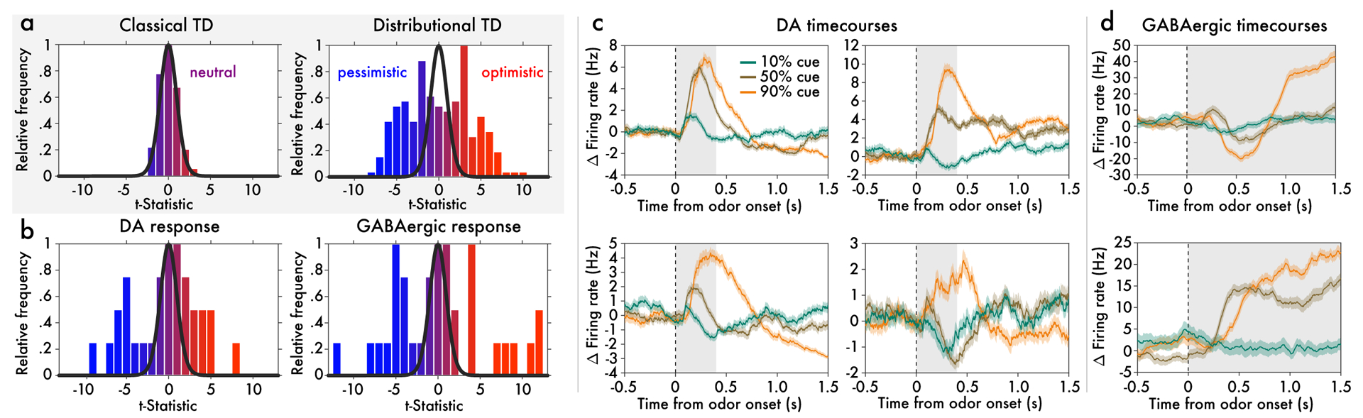
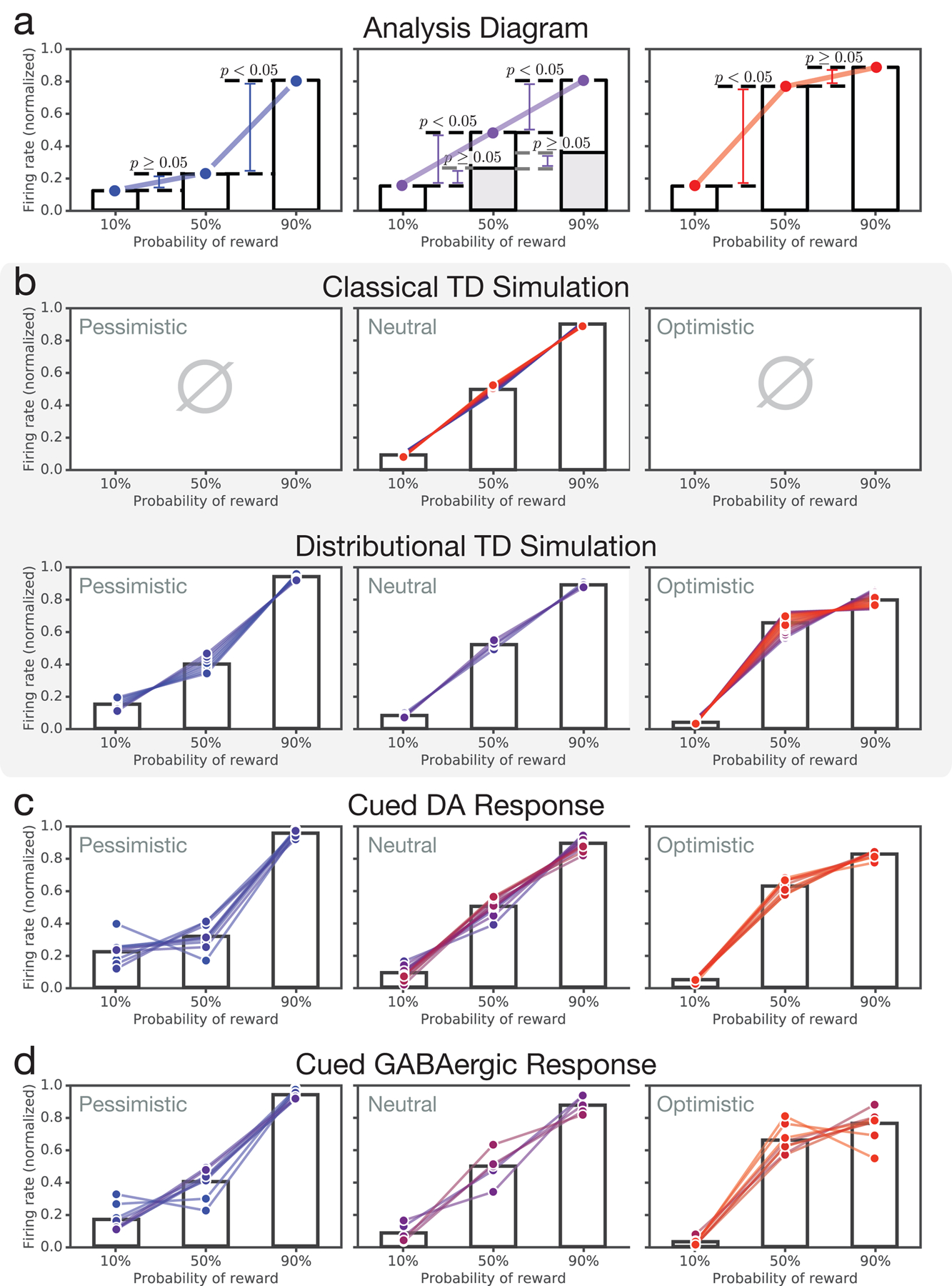
Data from variable-probability task. a, Histogram (across simulated cells) of t-statistics which compare each cell’s 50% cue response against the mean 50% cue response across cells. (Qualitatively identical results hold when comparing 50% cue response against midpoint of 10% and 90% responses.) The superimposed black curve shows the t-distribution with the corresponding degrees of freedom. Distributional TD predicts simultaneous optimistic and pessimistic coding of probability whereas classical TD predicts all cells have the same coding. Color indicates the degree of optimism or pessimism. b, Same as (a), but using data from real dopamine and putative GABA neurons. The pattern of results closely matches the predictions from the distributional TD model. c, Responses of four example dopamine neurons recorded simultaneously in a single animal. Each trace is the average response to one of the three cues. Time zero is the onset of the odor cue. Some cells code the 50% cue similarly to the 90% cue, while others simultaneously code it similarly to the 10% cue. Gray areas show epoch averaged for summary analyses. d, Responses of two example VTA GABAergic cells from the same animal.

To test this prediction, we analyzed responses of dopaminergic VTA neurons in the cued probability task just described (see Methods for more details). As predicted by distributional RL, but not by the standard theory, dopamine neurons differed in their patterns of response across the three reward-probability cues, with both optimistic and pessimistic probability coding observed (Figure 3b left and Extended Data Figures 6–7). Again, this diversity was not due to noise, as 10/31 cells were significantly optimistic and 9/31 were significantly pessimistic, at a p < 0.05 threshold (see Methods). By comparison, at a 0.05 threshold, approximately 3/31 cells in a non-distributional TD system are expected by chance to appear either significantly optimistic or pessimistic. At the group level, the null hypothesis of no diversity was rejected by one-way ANOVA (F(30, 3335) = 4.31, p = 6×10⁻¹⁴). Importantly, both forms of probability coding were observed side by side within individual animals. Within the animal with the greatest number of recorded cells, 4/17 cells were consistently optimistic and 5/17 cells were consistently pessimistic. This was also significant by ANOVA (F(15, 1652) = 4.02, p = 3 × 10⁻⁷).

Because most cells were recorded in different sessions, it was important to examine whether global changes in reward expectations between sessions might explain the observed diversity in optimism. To this end, we analyzed patterns of anticipatory licking. Here we found that, although within-session fluctuations in licking were predictive of within-session fluctuations in dopamine cell firing, there was no relationship between optimism and licking on a cell-by-cell basis (Extended Data Figure 9).

This observation makes it unlikely that the diverse responses we observed in dopamine neurons are explained by session-to-session variability in global reward expectation. That interpretation is further undermined by the fact that reversal-point diversity was observed in the one case where several cells were recorded simultaneously in one animal (Figure 3c and Supplement section 4).

VTA GABA neurons encode diverse reward predictions in parallel.

In distributional RL, diversity in RPE signaling arises because different RPE channels listen to different reward predictions, which vary in their degree of optimism. From a neuroscientific perspective, it should thus be possible to track the effects we have identified at the level of VTA dopamine neurons back to upstream neurons signalling reward predictions. Recent work strongly suggests that VTA GABAergic neurons play precisely this role, and that the reward prediction used to compute the RPE is reflected in their firing rates¹⁹. Therefore, we predicted that, in the same task described above, the population of VTA GABAergic neurons should also contain concurrent optimistic and pessimistic probability coding. As predicted, consistent differences in probability coding were observed across putative GABA neurons, again with concurrent optimism and pessimism (Figure 3b, right). In the animal with the most cells recorded, 12/36 cells were consistently optimistic, and 11/36 were consistently pessimistic (example cells shown in Figure 3d).

Distributional coding as a consequence of asymmetric RPE scaling.

The results reported in the preceding sections suggest that a distribution of value predictions is coded in the neural circuits underlying RL. But how might such coding arise in the first place? Recent AI work on distributional RL¹⁵ has shown that distributional coding arises automatically if a single change is made to the classic TD learning mechanism.

In classic TD, positive and negative errors are given equal weight. As a result, positive and negative errors are in equilibrium when the learned prediction equals the mean of the reward distribution. Therefore, classical TD learns to predict the average over future rewards.

By contrast, in distributional TD, different RPE channels place different relative weights on positive versus negative RPEs (see Figure 1b). In channels that overweight positive RPEs, reaching equilibrium requires these positive errors to become less frequent, so the learning dynamics converge on a more optimistic reward prediction. Conversely, in channels overweighting negative RPEs, a more pessimistic prediction is needed to attain equilibrium (Figure 4a and Extended Data Figure 1a). Taken together, the set of predictions learned across all channels encodes the full shape of the reward distribution.

Figure 4: Relative scaling of positive and negative dopamine responses predicts reversal point.

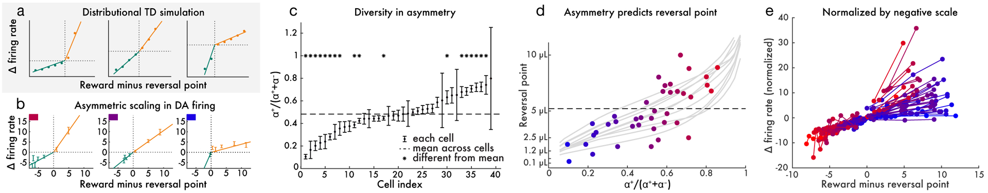
a, Three simulated dopamine neurons – each with a different asymmetry – in the variable-magnitude task. For each unit, we empirically estimated the reversal point where responses switch from negative to positive. The x-axis shows reward minus the per-cell reversal point, effectively aligning each cell’s responses to its respective reversal point. Baseline-subtracted response to reward is plotted on y-axis. Responses below the reversal point are shown in green and those above are shown in orange. Solid curves show linear functions fit separately to the above-reversal and below-reversal domains of each cell. b, Same as (a), but showing three real example dopamine cells. c, The diversity in relative scaling of positive and negative responses in dopamine cells is statistically reliable. The 95% confidence intervals of α⁺/(α⁺ + α⁻) are displayed, where α⁺ and α⁻ are the slopes estimated above. d, Relative scaling of positive and negative responses predicts that cell’s reversal point (each point is one dopamine cell). Dashed line is the mean over cells. Light gray traces show reversal points measured in distributional TD simulations of the same task, and show variability over simulation runs. e, All 40 dopamine cells plotted in the same fashion as in b, except normalized by the slope estimated in the negative domain. Thus, the observed variability in slope in the positive domain corresponds to diversity in relative scaling of positive and negative responses. Cells are colored by reversal point, to illustrate the relationship between reversal point and asymmetric scaling. In all panels, reward magnitudes are in estimated utility space (see Methods).

When distributional RL is considered as a model of the dopamine system, these points translate into two testable predictions. First, dopamine neurons should differ in their relative scaling of positive and negative RPEs. To test this prediction, we analyzed activity from VTA dopamine neurons in the variable-magnitude task described above. We first estimated a reversal point for each cell as previously described. Then, for each cell, we separately estimated two slopes: α⁺ for responses in the positive domain (i.e., above the reversal point) and α⁻ for the negative domain (Figure 4b). This revealed reproducible differences across dopamine neurons in the relative magnitude of positive versus negative RPEs (Extended Data Figure 5). Across all animals, the mean value of the ratio α⁺/(α⁺ + α⁻) was 0.48. However, many cells had a value significantly above or below this mean (Figure 4c; see Methods for details of statistical test). At the group level there was significant diversity between cells by one-way ANOVA (F(38, 234) = 2.93, p = 4 × 10⁻⁷). Within the animal with the most recorded cells, 3/15 cells were significantly below the mean and 3/15 were significantly above, and ANOVA again rejected the null hypothesis of no diversity between cells: F(14, 90) = 4.06, p = 2 × 10⁻⁵.

Second, RPE asymmetry should correlate, across dopamine neurons, with reversal point. Dopamine neurons that scale positive RPEs more steeply relative to negative RPEs should be linked with relatively optimistic reward predictions, and so should have reversal points at relatively high reward magnitudes. Dopamine neurons that scale positive RPEs less steeply should have relatively low reversal points. Again using data from the variable-magnitude task, we found a strong correlation between RPE asymmetry and reversal point (p = 8.1 × 10⁻⁵ by linear regression; Figure 4d,e), validating this prediction. Furthermore, this effect survived when only considering data from the single animal with the largest number of recorded cells (p = 0.002).

Decoding reward distributions from neural responses

As we have discussed, the distributional TD model correctly predicts that dopamine neurons should show diverse reversal points and response asymmetries, and that these should correlate. We last turn to the most detailed prediction of the model. The specific reversal points observed in any experimental situation, together with the particular response asymmetries in the corresponding neurons, should encode an approximate representation of the anticipated probability distribution over future rewards.

If this is in fact the case, then with sufficient data it should be possible to decode the the full value distribution from the responses of dopamine neurons. As a final test of the distributional RL hypothesis, we attempted this kind of decoding. The distributional TD model implies that, if dopaminergic responses are approximately linear in the positive and negative domains, then the resultant learned reward predictions will correspond to expectiles^* of the reward distribution³⁵.

We therefore treated the reversal points and response asymmetries measured in the variable-magnitude task as defining a set of expectiles, and we transformed these expectiles into a probability density (see Methods). As shown in Figure 5a–c, the resulting density captured multiple modes of the ground-truth value distribution. Decoding the RPEs produced by a distributional TD simulation, but not a classic TD simulation, produced the same pattern of results.

Figure 5: Decoding reward distributions from neural responses.

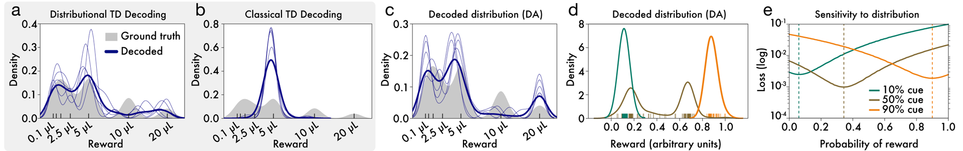
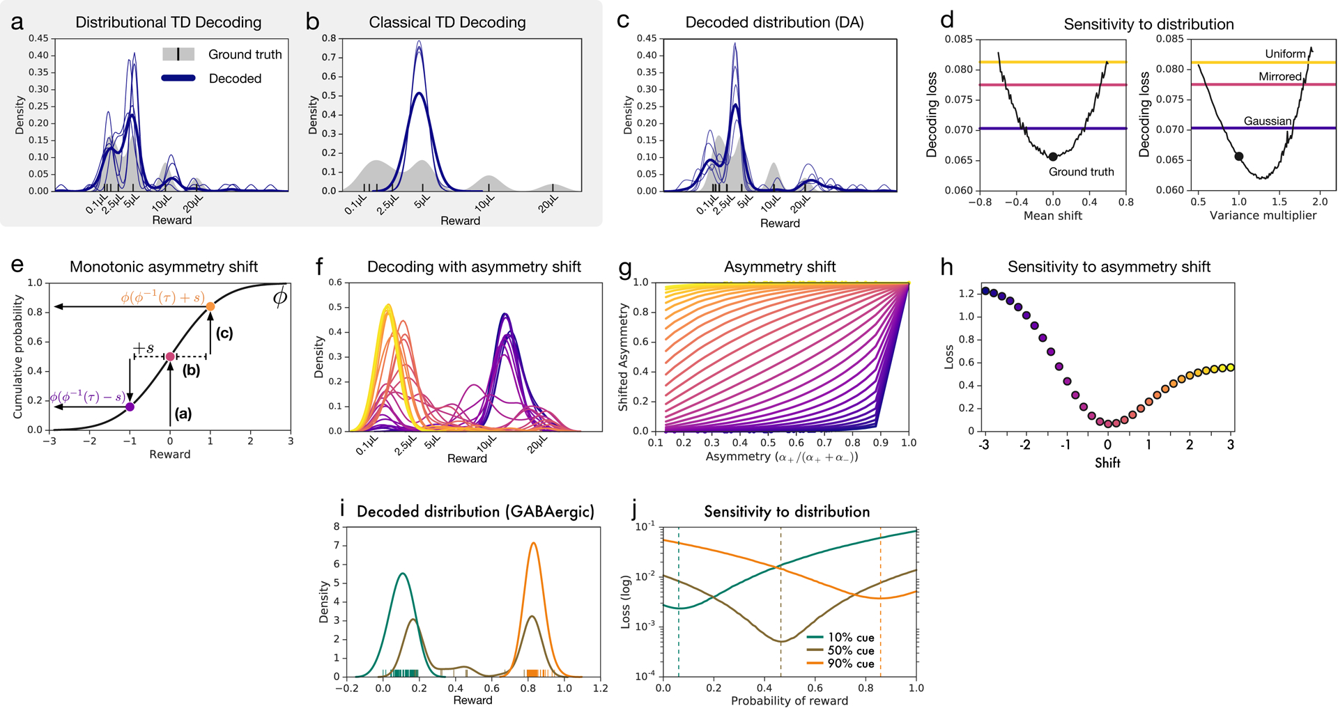
a, Distributional TD simulation trained on the variable-magnitude task, whose actual (smoothed) distribution of rewards is shown in gray. After training the model, we interpret the learned values as a set of expectiles. We then decode the set of expectiles into a probability density (blue traces). Multiple solutions are shown in light blue, and the average across solutions is shown in dark blue. (See Methods for more details.) b, Same as(a), but with a classical TD simulation. c, Same as (a), but using data from recorded dopamine cells. The expectiles are defined by the reversal points and the relative scaling from the slopes of positive and negative RPEs, as shown in Figure 5. Unlike the classic TD simulation, the real dopamine cells collectively encode the shape of the reward distribution that animals have been trained to expect. d Same decoding analysis, using data from each of the cue conditions in the variable-probability task, based on cue responses of dopamine neurons (decoding for GABA neurons shown in Extended Data Figure 8 i,j). e, The neural data for both dopamine and GABA neurons were best fit by Bernoulli distributions closely approximating the ground-truth reward probabilities in all three cue conditions.

Parallel analyses focusing on the variable-probability task (see Methods) yielded similarly good matches to the ground-truth distributions in that task (Figure 5d–e). In both tasks, successful decoding depended on the specific pattern of variability in the neural data, and not on the mere presence of variability per se (Extended Data Figure 8).

It is worth emphasizing that none of the effects we have reported are anticipated by the standard RPE theory of dopamine, which implies that all dopamine neurons should transmit essentially the same RPE signal. Why have the present effects not been observed before? In some cases, relevant data have been hiding in plain sight. For example, a number of studies have reported striking variability in the relative magnitude of positive and negative RPEs across dopamine neurons, treating this however as an incidental finding or a reflection of measurement error, or viewing it as a problem for the RPE theory¹⁷. And one of the earliest studies of reward-probability coding in dopaminergic RPEs remarked on apparent diversity across dopamine neurons, though only in a footnote¹⁸. A more general issue is that the forms of variability we have reported are masked by traditional analysis techniques, which typically focus on average responses across dopamine neurons (see Supplement section 5 and Extended Data Figure 10).

Distributional RL offers a range of untested predictions. Dopamine neurons should maintain their ordering of relative optimism across task contexts, even as the specific distribution of rewards changes. If RPE channels with particular levels of optimism are selectively activated with optogenetics, this should sculpt the learned distribution, which should in turn be detectable with behavioral measures of sensitivity to moments of the distribution. We list further predictions in Supplement section 6.

Distributional RL also gives rise to a number of broader questions. What are the circuit- or cellular-level mechanisms that give rise to a diversity of asymmetry in positive versus negative RPE scaling? It is also worth considering whether other mechanisms, aside from asymmetric scaling of RPEs, might contribute to distributional coding. It is well established, for example, that positive and negative RPEs differentially engage striatal D1 and D2 receptors²⁰, and that the balance of these receptors varies anatomically^21–23. This suggests a second potential mechanism for differential learning from positive versus negative RPEs²⁴. Also, how do different RPE channels anatomically couple with their corresponding reward predictions (see Extended Data Figure 4i–k)? Finally, what effects might distributional coding have downstream, at the level of action learning and selection? With this question in mind, it is interesting to note that some current theories in behavioral economics center on risk measures that can be easily read out from the kind of distributional codes that the present work has considered.

We close by speculating on implications of the distributional hypothesis of dopamine for the mechanisms of mental disorders such as addiction and depression. Mood has been linked with predictions of future reward²⁵, and it has been proposed that both depression and bipolar disorder may involve biased forecasts concerning value-laden outcomes²⁶. Of obvious relevance, it has recently been proposed that such biases may arise from asymmetries in RPE coding^27,28. Potential connections between these ideas and the phenomena we have reported here are readily evident, presenting novel and inviting opportunities for new research.

Methods

Distributional reinforcement learning model

The model for distributional reinforcement learning (distributional RL) we use throughout the work is based on the principle of asymmetric regression and extends recent results in AI^5,6,15. We present a more detailed and accessible introduction to distributional RL in the Supplement. Here we outline the method in brief.

Let $f:ℝ\to ℝ$ be a response function. In each observed state x, let there be a set of value predictions V_i(x) which are updated with learning rates ${\alpha }_i^{+},{\alpha }_i^{-}\in {ℝ}^{+}$. Then given a state x, next-state x′, resulting reward signal r, and time-discount γ ∈ [0, 1) the distributional TD model computes distributional TD errors

$${\delta }_i=r+\gamma V_i\left(x^{\prime }\right)-V_i\left(x\right),$$ (1)

where V_j(x′) is a sample from the distribution V (x′). The model then updates the baselines with

$$V_i\left(x\right)\leftarrow V_i\left(x\right)+{\alpha }_i^{+}f\left({\delta }_i\right)\text{for}{\delta }_i>0$$ (2)

$$V_i\left(x\right)\leftarrow V_i\left(x\right)+{\alpha }_i^{-}f\left({\delta }_i\right)\text{for}{\delta }_i\le 0$$ (3)

When performed with a tabular representation, asymmetry uniformly distributed, and f(δ) = sign(δ), this method converges to the τ_i-quantile, ${\tau }_i=\frac{{\alpha }_i^{+}}{{\alpha }_i^{+}+{\alpha }_i^{-}}$, of the distribution over discounted returns at x⁶. Similarly, asymmetric regression with response function f(δ) = δ corresponds to expectile regression²⁹. Like quantiles, expectiles fully characterize the distribution and have been shown to be particularly useful for measures of risk^30,31.

Finally, we note that throughout the paper, we use the terms ‘optimistic’ and ‘pessimistic’ to refer to return predictions that are above or below the mean (expected) return. Importantly, these predictions are optimistic in the sense of corresponding to particularly good outcomes from the set of possible outcomes. They are not optimistic in the sense of corresponding to outcomes that are impossibly good.

Artificial agent results

Atari results are on the Atari-57 benchmark using the publicly available Arcade Learning Environment³². This is a set of 57 Atari 2600 games and human-performance baselines. Refer to previous work for details on DQN and computation of human-normalized scores⁸. The Distributional TD agent uses our proposed model and a DQN with multiple (n = 200) value predictors, each with a different asymmetry, spaced uniformly in [0, 1]. The training objective of DQN, the Huber loss, is replaced with the asymmetric quantile-Huber loss, which corresponds to the κ-saturating response function f(δ) = max(min(δ, κ), −κ), with κ = 1.

Finally, at each update we train all channels based upon the immediate reward and the predicted future returns from all next-state value predictors. Further details can be found in Dabney et al.⁶. The physics-based motor-control task requires control of a 28 degrees-of-freedom humanoid to complete a 3-dimensional obstacle course in minimal time³³. Full details for the D3PG and Distributional D3PG agents are given in Barth-Maron et al.¹⁴. Distributions over return shown in Extended Data Figure 2d and 2f are based on the network-predicted distribution in each of the given frames.

Tabular simulations

Tabular simulations of the classical TD and distributional TD models used a population of learning rates selected uniformly at random, ${\alpha }_i^{+}~u\left(0,1\right)$ for each cell i. In all cases the only algorithmic difference between the classical and distributional TD models was that the distributional model used a separately varying learning rate for negative prediction errors, ${\alpha }_i^{-}~u\left(0,1\right)$ for each cell i. Both methods used a linear response function. Qualitatively similar results were also obtained with other response functions (e.g. Hill function³⁴ or κ – saturating), despite these leading to semantically different estimators of the distribution. The population sizes were chosen for clarity of presentation and to provide similar variability as observed in the neuronal data. Each cell was paired with a different state-dependent value estimate V_i(x). Note that while these simulations focused on immediate rewards, the same algorithm also learns distributions over multi-step returns.

In the variable-probability task, each cue corresponded to a different value estimate and reward probability (90%, 50%, or 10%). When rewarded, the agent received numerical reward of 1.0, and 0.0 when omitted. Both agents were trained for 100 trials of 5000 updates, and both simulated n = 31 cells (separate value estimates). The learning rates were all selected uniformly at random between [0.001, 0.2]. Cue response was taken to be the temporal difference from a constant zero baseline to the value estimate.

In the variable-magnitude task, all rewards were taken to be the water magnitude measured in micro-liters (qualitatively same results obtained with utilities instead of magnitudes). For Figure 2 we ran 10 trials of 25000 updates each for 150 estimators with random learning rates in [0.001, 0.02]. These smaller learning rates and larger number of updates were intended to ensure the values converged fully with low error. We then report temporal difference errors for 10 cells taken uniformly to span the range of value estimates for each agent. Reported errors (simulating change in firing rate) are the utility of a reward minus the value estimate and scaled by the learning rate. As with the neuronal data, these are reported averaged over trials and normalized by variance over reward magnitudes. Distributional TD RPEs are computed using asymmetric learning rates, with a small constant (floor) added to the learning rates.

Distribution decoding

For both real neural data and TD simulations, we performed distribution decoding. The distributional and classic TD simulations used for decoding in the variable-magnitude task each employed 40 value predictors, to match the 40 recorded cells in the neural data (neural analyses were pooled across the six animals). In the distributional TD simulation, each value predictor used a different asymmetric scaling factor ${\tau }_i={\alpha }_i^{+}/\left({\alpha }_i^{+}+{\alpha }_i^{-}\right)$, and therefore learned a different value prediction V_i.

The decoding analyses began with a set of reversal points, V_i, and asymmetric scaling factors τ_i. For the neural data, these were obtained as described elsewhere. For the simulations, they were read directly from the simulation. These numbers were interpreted as a set of expectiles, with the τ_i-th expectile having value V_i. We decoded these into probability densities by solving an optimization problem to find the density most compatible with the set of expectiles³⁵. For optimization, the density was parameterized as a set of samples. For display in Figure 5, the samples are smoothed with kernel density estimation.

Animals and behavioral tasks

The rodent data we re-analyzed here were first reported in Eshel et al.¹⁹. Methods details can be found in that paper and in Eshel et al.³⁴. We give a brief description of the methods below.

Five mice were trained on a ‘variable-probability’ task, and six different mice on a ‘variable-magnitude’ task. In the variable-probability task, in each trial the animal first experienced one of four odor cues for 1 s, followed by a 1 s pause, followed by either a reward (3.75 μL water), an aversive airpuff, or nothing. Odor 1 signaled a 90% chance of reward, odor 2 a 50% chance of reward, odor 3 a 10% chance of reward, and odor 4 signaled a 90% chance of airpuff. Odor meanings were randomized across animals. Inter-trial intervals were exponentially distributed.

An infrared beam was positioned in front of the water delivery spout, and each beam break was recorded as one lick event. We report the average lick rate over the entire interval between the cue and the outcome (i.e., 0–2000 ms after cue onset).

In the variable-magnitude task, in 10% of trials an odor cue was delivered that indicated that no reward would be delivered on that trial. In the remaining 90% of trials, one of the following reward magnitudes was delivered, at random: 0.1, 0.3, 1.2, 2.5, 5, 10, 20 μL. In half of these trials, this reward was preceded 1500 ms by an odor cue (which indicated that a reward was forthcoming but did not disclose its magnitude). In the other half, it was unsignalled.

In order to identify dopamine neurons while recording, neurons in the VTA were tagged with channelrhodopsin-2 (ChR2) by injecting adeno-associated virus (AAV) that expresses ChR2 in a Cre-dependent manner into the VTA of transgenic mice that express Cre recombinase under the promotor of the dopamine transporter (DAT) gene (B6.SJL-Slc6a3tm1.1(cre)Bkmn/J, The Jackson Laboratory)³⁶. Mice were implanted with a head plate and custom-built microdrive containing 6–8 tetrodes (Sandvik) and optical fiber, as described in Cohen et al.³⁷.

All experiments were performed in accordance with the US National Institutes of Health Guide for the Care and Use of Laboratory Animals and approved by the Harvard Institutional Animal Care and Use Committee.

Neuronal data and analysis

Extracellular recordings were made from VTA using a data acquisition system (DigiLynx, Neuralynx). VTA recording sites were verified histologically. The identity of dopaminergic cells was confirmed by recording the electrophysiological responses of cells to a brief blue light pulse train, which stimulates only DAT-expressing cells. Spikes were sorted using Spike-Sort3D (Neuralynx) or MClust-3.5 (A.D. Redish). Putative GABAergic neurons in the VTA were identified by clustering of firing patterns as described previously^34,37. All confidence intervals are standard error unless otherwise noted.

Data analyses were performed using NumPy 1.15 and MATLAB R2018a (Mathworks). Spike times were collected in 1 ms bins to create peri-stimulus time histograms. These histograms were then smoothed by convolving with the function

$$\left(1-e^{-t}\right)\cdot e^{-t/T}$$

where T was a time constant, set to 20 ms as in Eshel et al.³⁴. For single-cell traces, we set T to 200 ms for display purposes.

After smoothing, the data were baseline-corrected by subtracting from each trial and each neuron independently the mean over that trial’s activity from −1000 to 0 ms relative to stimulus onset (or relative to reward onset in the unexpected reward condition).

Variable-probability task

n = 31 cells were recorded from five animals, with the following number of cells per animal: 1, 4, 16, 1, 9. Responses to cue for dopamine neurons were defined as the average activity from 0 to 400 ms after cue onset. This interval was chosen to match Eshel et al.³⁴. Responses to cue for putative GABA neurons were defined as the average activity from 0 to 1500 ms after cue onset. This longer interval was chosen because these neurons had much slower responses, often ramping up slowly over the first 500 or 1000 ms after cue onset³⁷ (Figure 3d).

We were interested in whether there was between-cell diversity in responses to the 50% cue. We first normalized the responses to the 50% cue on a per-cell basis as follows:

$$c_{50}^{\mathit{\text{norm}}}=\left(c_{50}-\mathit{\text{mean}}\left(c_{10}\right)\right)/\left(\mathit{\text{mean}}\left(c_{90}\right)-\mathit{\text{mean}}\left(c_{10}\right)\right)$$

where mean indicates the mean over trials within a cell. In order to be agnostic about the risk preferences of the animal, we then performed a two-tailed t-test of the cell’s normalized responses to the 50% cue against the average of all cells’ normalized responses to the 50% cue. This is the test for optimistic or pessimistic probability coding that we report in the main text. Note that these t-statistics would be t-distributed if the differences between cells were due to chance. We also report ANOVA results where we evaluate the null hypothesis that all cells’ normalized 50% responses have the same mean.

The same pattern of results held when instead comparing responses to the 50% cue against the midway point between responses to the 10% cue and responses to the 90% cue.

The per-cell cue responses shown in Extended Data Figure 7 were normalized to zero mean and unit variance, to allow direct comparison of cells with different response variability. Each cell appears in one of three panels based upon the outcome of two single-tailed Mann-Whitney tests evaluating the rank order for c₁₀ < c₅₀ and c₅₀ < c₉₀ (see Supplement section 3.3 for further details). The left, center, and right panels correspond to outcomes (p ≥ 0.05, p < 0.05), (p < 0.05, p < 0.05 or p ≥ 0.05, p ≥ 0.05), and (p < 0.05, p ≥ 0.05) respectively.

Variable-magnitude task

n = 40 cells were recorded from five animals, with the following number of cells per animal: 3, 6, 9, 16, 6. Responses to reward were defined as the average activity from 200 to 600 ms after reward onset. This time interval was selected to match Eshel et al.³⁴ as closely as possible, while excluding the initial response to the feeder click^34,38,39, which was not selective to reward magnitude and was positive for all reward magnitudes. This allowed us to find the reward magnitudes for which the dopamine response was either boosted or suppressed relative to baseline.

The reversal point (i.e., the reward magnitude that would elicit neither a positive nor negative deflection in firing relative to baseline) for each cell was defined as the magnitude M_R that maximized the number of positive responses to rewards greater than M_R plus the number of negative responses to rewards less than M_R. To obtain statistics for reliability of cell-to-cell differences in reversal point, we partitioned the data into random halves and estimated the reversal point for each cell separately in each half. We repeated this procedure 1000 times with different random partitions, and we report the mean R value and geometric mean p value across these 1000 folds.

After measuring reversal points, we fit linear functions separately to the positive and negative domains of each cell. To obtain confidence intervals, we divided the data into seven random partitions (seven being the smallest number of trials in any condition for any cell), subject to the constraint that every condition for every cell contain at least one trial in each partition. In each partition, we repeated the procedure for estimating reversal points and finding slopes in the positive and negative domains. Our confidence interval on τ = α⁺/(α⁺ + α⁻) was then the SEM of the values calculated across the seven partitions. ANOVAs are also reported testing the null hypothesis that means (across partitions) were not different between cells.

Fitting linear functions to dopamine responses was more logical in utility space than in reward volume space. We relied on Stauffer et al.³⁸ to approximate the underlying utility function from the dopamine responses to rewards of varying magnitudes. We used these empirical utilities instead of raw reward magnitudes for the analyses shown in Figure 4. However, none of the reported results were sensitive to this choice of utility function. We also ran the analyses using other utility functions, and these results are reported in Extended Data Figure 5. One cell was excluded from analyses in Figure 5: because it had no positive responses to any reward magnitude, a slope could not be fit in the positive domain.

When measuring the correlation (across cells) between reversal point and τ, we first randomly split the data into two disjoint halves of trials. In one half, we first calculated reversal points RP₁ and used these reversal points to calculate α⁺ and α⁻. In the other half, we calculated reversal points RP₂. The correlation we report is between RP₂ and τ = α⁺/(α⁺ + α⁻). We did this to avoid confounds associated with using the same data to estimate both slopes and intercepts.

Data and code availability

The neuronal data analyzed in this work, along with analysis code from our value-distribution decoding and code used to generate model predictions for distributional TD are available at https://doi.org/10.17605/OSF.IO/UX5RG.

Extended Data

Extended Data Figure 1: Mechanism of distributional TD.

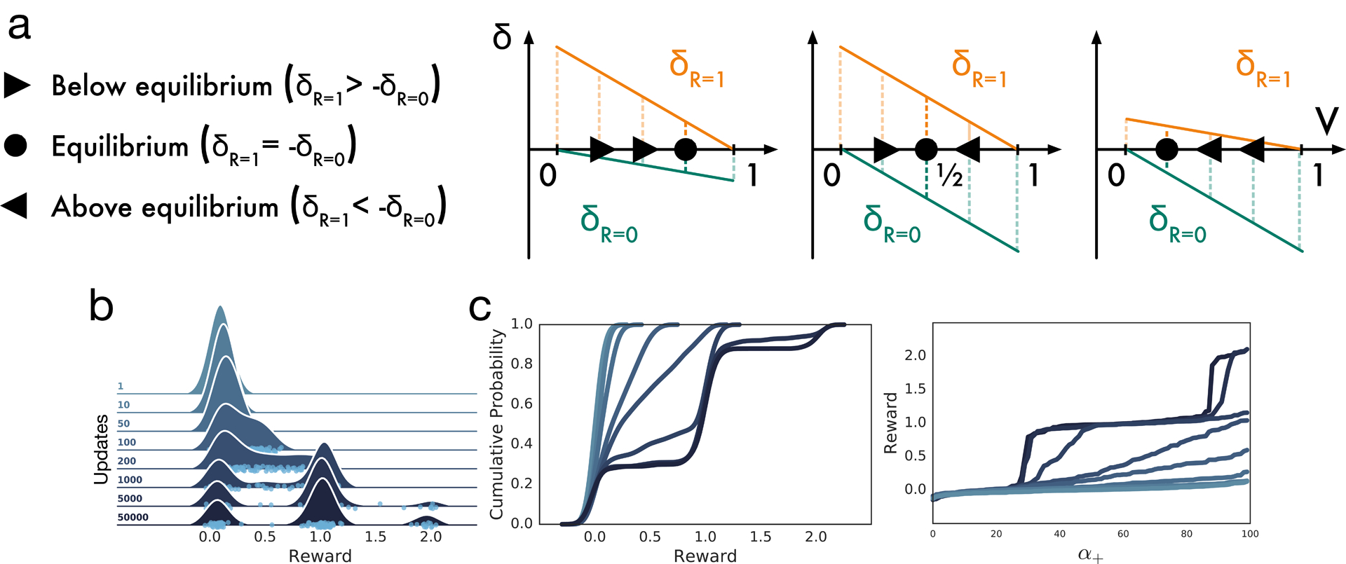
a, The degree of asymmetry in positive to negative scale determines the equilibrium where positive and negative errors balance. Equal scaling equilibrates at the mean, whereas a larger positive (negative) scaling produces an equilibrium above (below) the mean. b, Distributional prediction emerges through experience. Quantile (sign function) version is displayed here for clarity. Model is trained on arbitrary task with trimodal reward distribution. c, Same as (b), viewed in terms of cumulative distribution (left) or learned value for each predictor (quantile function) (right).

Extended Data Figure 2: Learning the distribution of returns improves performance of deep RL agents across multiple domains.

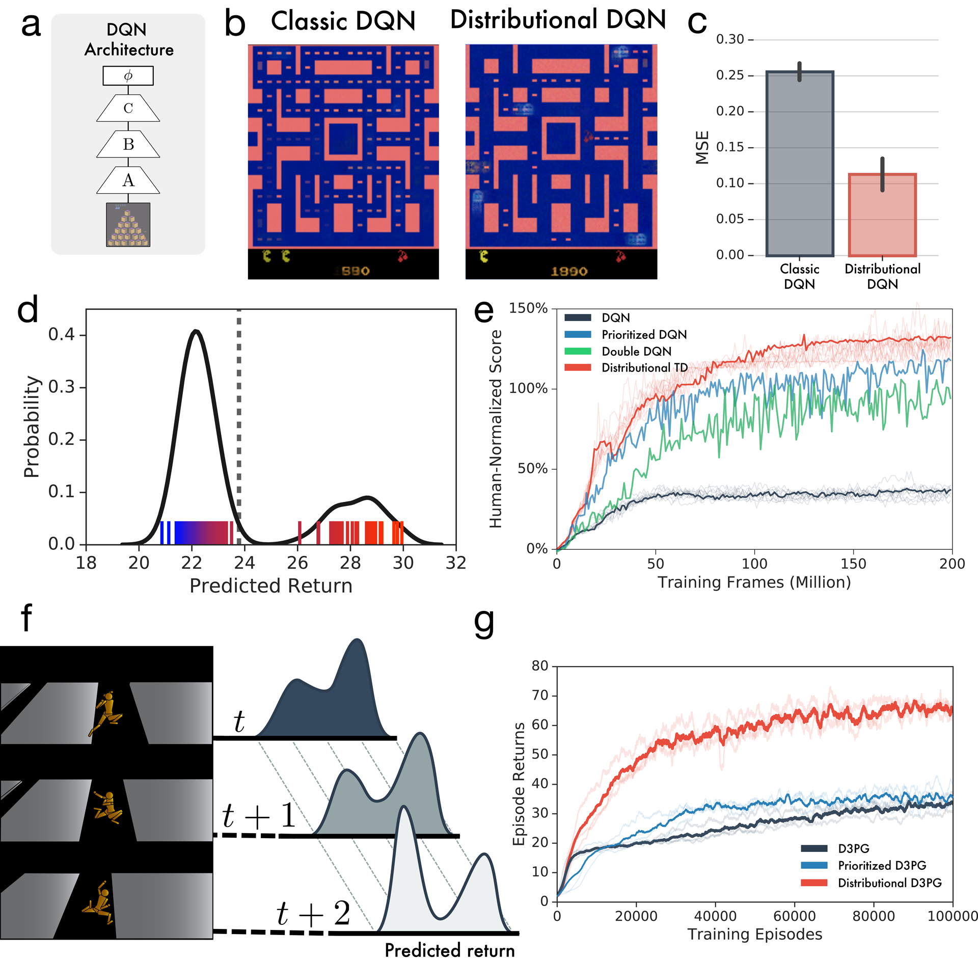
a, DQN and Distributional TD share identical non-linear network structures. b-c, After training classic or distributional DQN on MsPacman, we freeze the agent and then train a separate linear decoder to reconstruct frames from the agent’s final layer representation. For each agent, reconstructions are shown. The distributional model’s representation allows significantly better reconstruction. d, At a single frame of MsPacman (not shown), the agent’s value predictions together represent a probability distribution over future rewards. Reward predictions of individual RPE channels shown as tick marks ranging from pessimistic (blue) to optimistic (red), and kernel density estimate shown in black. e, Atari-57 experiments with single runs of prioritized experience replay⁴⁰ and double DQN⁴¹ agents for reference. Benefits of distributional learning exceed other popular innovations. f-g, The performance payoff of distributional RL can be seen across a wide diversity of tasks. Here we give another example, a humanoid motor-control task in the MuJoCo physics simulator. Prioritized experience replay agent is shown for reference.⁴² Traces show individual runs, averages in bold.

Extended Data Figure 3: Simulation experiment to examine the role of representation learning in distributional RL.

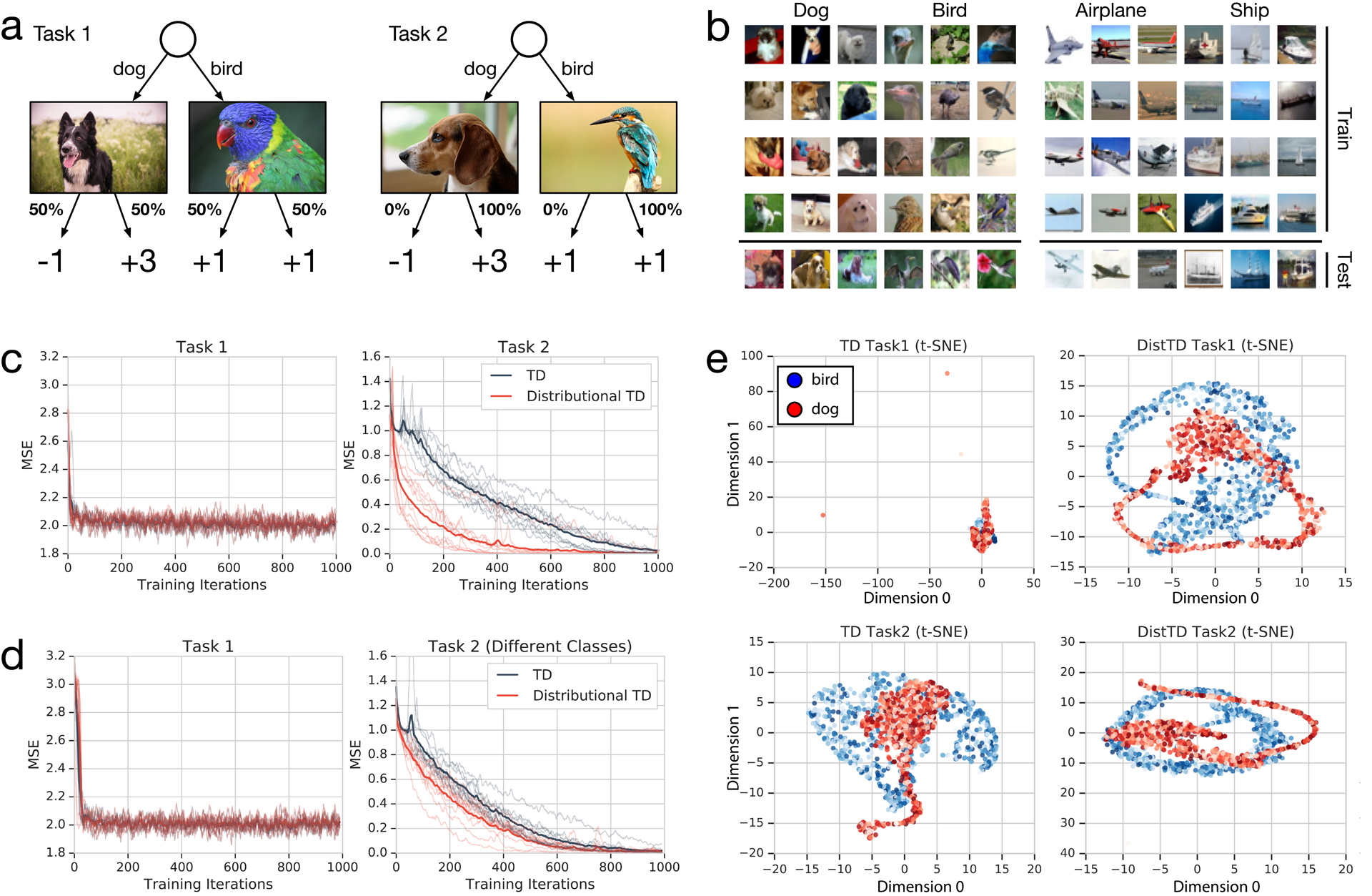
a, Illustration of tasks 1 and 2. b, Example images for each class used in our experiments. c, Experimental results, where each of 10 random seeds yields an individual run shown with traces, and bold gives average over seeds. d, Same as (c), but for control experiment. e, Bird-dog t-SNE visualization of final hidden layer of network, given different input images (bird=blue, dog=red). Left column shows classic TD and right column shows distributional TD. Top row shows the representation after training on task 1, and bottom row after training on task 2.

Extended Data Figure 4: Null models.

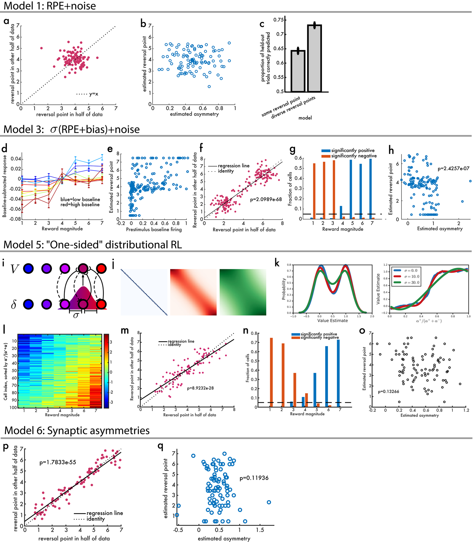
a, Classical TD plus noise does not give rise to the pattern of results observed in real dopamine data in varible-magnitude task. When reversal points were estimated in two independent partitions there was no correlation between the two (p=0.32 by linear regression). b, We then estimated asymmetric scaling of responses and found no correlation between this and reversal point (p=0.78 by linear regression). c, Model comparison between ‘same’, a single reversal point, and ‘diverse’, separate reversal points. In both, the model is used to predict whether a held-out trial has a positive or negative response. d, Simulated baseline-subtracted RPEs, color-coded according to the ground-truth value of bias added to that each cell’s RPEs. e, Across all simulated cells, there was a strong positive relationship between prestimulus baseline firing and the estimated reversal point. f, Two independent measurements of the reversal point were strongly correlated. g, The proportion of simulated cells that have significantly positive (blue) or negative (red) responses showed no magnitudes with both positive and negative responses. h, In the simulation, there was a significant negative relationship between the estimated asymmetry of each cell and its estimated reversal point (opposite that observed in neural data). i, Diagram illustrating a Gaussian weighted topological mapping between RPEs and value predictors. j, Varying the standard deviation of this Gaussian modulates the degree of coupling. k, In a task with equal chance of a reward 1.0 or 0.0, distributional TD with different levels of coupling shows robustness to the degree of coupling. l, When there is no coupling, a distributional code is not learned, but asymmetric scaling can cause spurious detection of diverse reversal points. m, Even though every cell has the same reward prediction they appear to have different reversal points. n, With this model, some cells may have significantly positive responses, and others significantly negative responses, in response to the same reward. o, But this model is unable to explain a positive correlation between asymmetric scaling and reversal points. p, Simulation of “synaptic” distributional RL, where learning rates but not firing rates are asymmetrically scaled. This model predicts diversity in reversal points between dopamine neurons. q, But it predicts no correlation between asymmetric scaling of firing rates, and reversal point.

Extended Data Figure 5: Asymmetry and reversal.

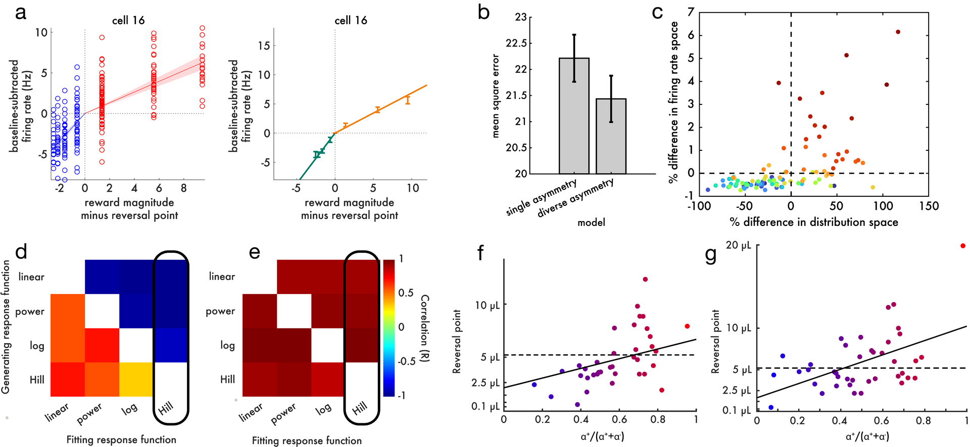
a, Left, All data points (trials) from an example cell. The solid lines are linear fits to the positive and negative domains, and the shaded areas show 95% confidence intervals calculated with Bayesian regression. Right, the same cell plotted in the format of main text Figure 4b. b, Cross-validated model comparison on the dopamine data favors allowing each cell to have its own asymmetric scaling (p = 1.4e – 11 by paired t-test). The standard error of the mean appears large relative to the p-value because the p-value is computed using a paired test. c, Although the difference between single-asymmetry and diverse-asymmetry models was small in firing rate space, such small differences correspond to large differences in decoded distribution space (more details in Supplement). Each point is a TD simulation; color indicates the degree of diversity in asymmetric scaling within that simulation. d, We were interested in whether an apparent correlation between reversal point and asymmetry could arise as an artifact, due to a mismatch between the shape of the actual dopamine response function and the function used to fit it. Here we simulate the variable-magnitude task using a TD model without a true correlation between asymmetric scaling and reversal point. We then apply the same analysis pipeline as in the main paper, to measure the correlation (color axis) between asymmetric scaling and reversal point. We repeat this procedure 20 times with different dopamine response functions in the simulation, and different functions used to fit the positive and negative domains of the simulated data. The functions are sorted in increasing order of concavity. An artifact can emerge if the response function used to fit the data is less concave than the response function used to generate the data. For example, when generating data with a Hill function but fitting with a linear function, a positive correlation can be spuriously measured. e, When simulating data from the distributional TD model, where a true correlation exists between asymmetric scaling and reversal point, it is always possible to detect this positive correlation, even if the fitting response function is more concave than the generating response function. The black rectangle highlights the function used to fit real neural data in panel c. f, In this panel we analyze the real dopamine cell data identically to main text Figure 4d, but using Hill functions instead of linear functions to fit the positive and negative domains. Because the correlation between asymmetric scaling and reversal point still appears under these adversarial conditions, we can be confident it is not driven by this artifact. g, Same as main text Figure 4d, but using linear response function and linear utility function (instead of empirical utility).

Extended Data Figure 6: Cue responses versus outcome responses, and more evidence for diversity.

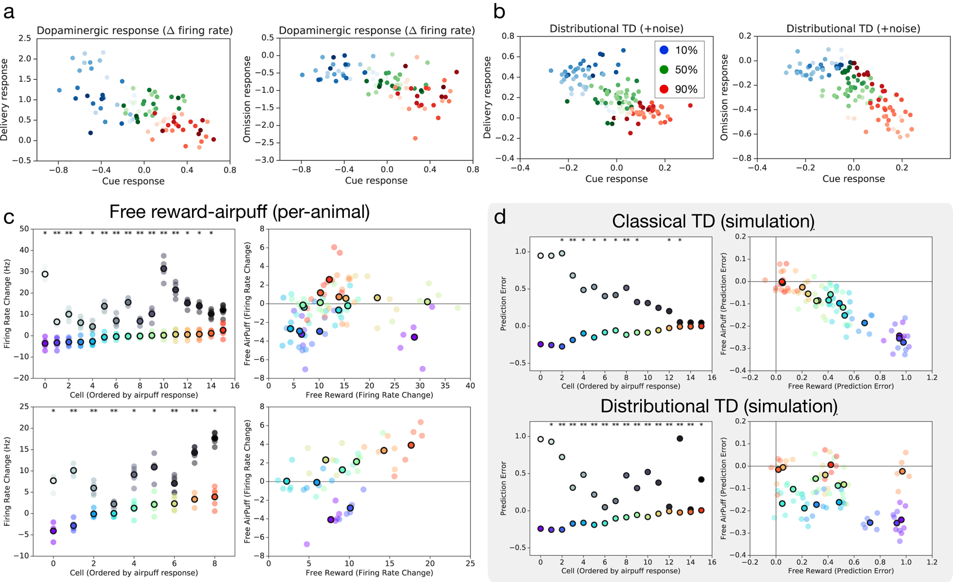
a, In variable-probability task: firing at cue, versus firing at reward (left) or omission (right). Color brightness denotes asymmetry. b, Same as (a), but showing RPEs from distributional TD simulation. c, Data from Eshel et al.³⁴ also included unpredicted rewards and unpredicted airpuffs. Top two panels show responses for all the cells recorded in one animal and bottom two panels show responses for all the cells of another animal. In the left two panels, the x-axis is the baseline-subtracted response to free reward, and the y-axis is the baseline-subtracted response to airpuff. Dots with black outlines are per-cell means, and un-outlined dots are means of disjoint subsets of trials indicating consistency of asymmetry. The right two panels plot the same data in a different way, with cells sorted along the x-axis by response to airpuff. Response to reward is shown in grayscale dots. Asterisks indicate significant difference in firing rates from one or both neighboring cells. d, Simulations for distributional but not classical TD produce diversity in relative response.

Extended Data Figure 7: More details of data in variable-probability task.

a, Details of analysis method. Of the four possible outcomes of the two Mann-Whitney tests (described in Methods), two outcomes correspond to interpolation (middle) and one each to the pessimistic (left) and optimistic (right) groups. b, Simulation results for the classical TD and distributional TD models. Y-axis shows the average firing rate change, normalized to mean zero and unit variance, in response to each of the three cues. Each curve is one cell. The cells are split into panels according to a statistical test for type of probability coding (see Methods for details). Color indicates the degree of optimism or pessimism. Distributional TD predicts simultaneous optimistic and pessimistic coding of probability whereas classical TD predicts all cells have the same coding. c, Same as b, but using data from real dopamine neurons. The pattern of results closely matches the predictions from the distributional TD model. d, Same as b, using data from putative VTA GABAergic interneurons.

Extended Data Figure 8: Further distribution decoding analysis.

This figure pertains to the variable-magnitude experiment. a-c, In the decoding shown in the main text, we constrained the support of the distribution to the range of the rewards in the task. Here, we applied the decoding analysis without constraining the output values. We find similar results, although with increased variance. d, We compare the quality of the decoded distribution against several controls. The real decoding is shown as black dots. In colored lines are reference distributions (uniform and Gaussian with the same mean and variance as the ground truth; and the ground truth mirrored). Black traces shift or scale the ground truth distribution by varying amounts. e, Nonlinear functions used to shift asymmetries, to measure degradation of decoded distribution. The normal cumulative distribution function ϕ is used to transform asymmetry τ. This is shifted by some value s and transformed back through the normal quantile function ϕ⁻¹. Positive values s increase the value of τ and negative values decrease the value of τ. f, Decoded distributions under different shifts, s. g, Plot of shifted asymmetries for values of s used. h, Quantification of match between decoded and ground truth distribution, for each s. i-j, Same as main text Figure 5d–e, but for putative GABAergic cells rather than dopamine cells.

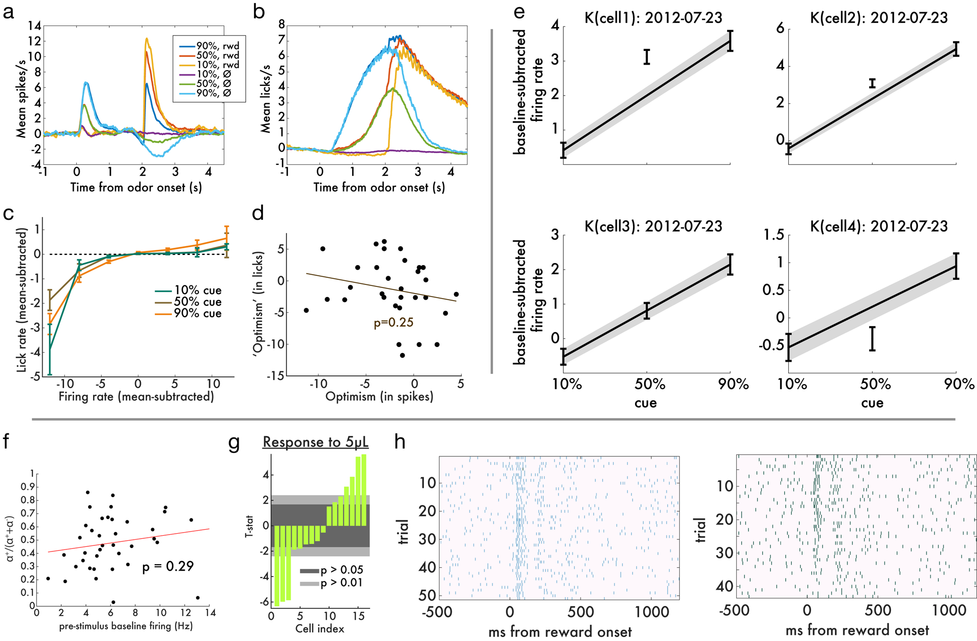
Extended Data Figure 9: Simultaneous diversity.

Variable-probability task. Mean spiking (a) and licking (b) activity in response to each of the three cues (indicating 10%, 50% or 90% probability of reward) at time 0, and in response to the outcome (reward or no reward) at time 2000 ms. c, Trial-to-trial variations in lick rates were strongly correlated with trial-to-trial variations in dopamine firing rates. Each cell’s mean is subtracted from each axis, and the x-axis is binned for ease of visualization. d, Dopaminergic coding of the 50% cue relative to the 10% and 90% cues (as shown in panel b) was not correlated with the same measure computed on lick rates. Therefore, between-session differences in cue preference, measured by anticipatory licking, cannot explain between-cell differences in optimism. e, Four simultaneously recorded dopamine neurons. These are the same four cells whose timecourses are shown in Figure 3c in the main text. f, Variable-magnitude task. Across cells, there was no relationship between asymmetric scaling of positive versus negative prediction errors, and baseline firing rates (R=0.18, p=0.29). Each point is a cell. These data are from dopamine neurons at reward delivery time. g, t-statistics of response to 5 μL reward compared to baseline firing rate, for all 16 cells from animal ‘D’. Some cells respond significantly above baseline and others significantly below. Cells are sorted by t-statistic. h, Spike rasters showing all trials where the 5 μL reward was delivered. The two panels are two example cells from the same animal with rasters shown in Figure 2 of the main text.

Extended Data Figure 10: Relationship of results to Eshel et al (2016).

Here we reproduce results for the variable-magnitude task from Eshel et al.³⁴ with two different time windows. a, Change in firing rate in response to cued reward delivery averaged over all cells. b, Comparing hill-function fit and response averaged over all cells for expected (cued) and unexpected reward delivery. c, Correlation between response predicted by scaled common response function and actual response to expected reward delivery. d, Zooming in on (c) shows correlation driven primarily by larger reward magnitudes. e-h, Repeating the above analysis for a window of 200 – 600ms.

References

- 1.Schultz Wolfram, Wiliam R Stauffer, and Armin Lak. The phasic dopamine signal maturing: from reward via behavioural activation to formal economic utility. Current opinion in neurobiology, 43: 139–148, 2017. [DOI] [PubMed] [Google Scholar]
- 2.Glimcher Paul W. Understanding dopamine and reinforcement learning: the dopamine reward prediction error hypothesis. Proceedings of the National Academy of Sciences, 108(Supplement 3):15647–15654, 2011. [DOI] [PMC free article] [PubMed] [Google Scholar]
- 3.Watabe-Uchida Mitsuko, Eshel Neir, and Uchida Naoshige. Neural circuitry of reward prediction error. Annual review of neuroscience, 40:373–394, 2017. [DOI] [PMC free article] [PubMed] [Google Scholar]
- 4.Morimura Tetsuro, Sugiyama Masashi, Kashima Hisashi, Hachiya Hirotaka, and Tanaka Toshiyuki. Parametric return density estimation for reinforcement learning In Proceedings of the Twenty-Sixth Conference on Uncertainty in Artificial Intelligence, UAI’10, pages 368–375, Arlington, Virginia, United States, 2010. AUAI Press; ISBN 978-0-9749039-6-5. URL http://dl.acm.org/citation.cfm?id=3023549.3023592. [Google Scholar]
- 5.Marc G Bellemare Will Dabney, and Munos Rémi. A distributional perspective on reinforcement learning. In International Conference on Machine Learning, pages 449–458, 2017. [Google Scholar]
- 6.Dabney Will, Rowland Mark, Bellemare Marc G, and Munos Rémi. Distributional reinforcement learning with quantile regression. AAAI Conference on Artificial Intelligence, 2018. [Google Scholar]
- 7.Sutton Richard S and Barto Andrew G. Reinforcement learning: an introduction, volume 1 MIT press Cambridge, 1998. [Google Scholar]
- 8.Mnih Volodymyr, Kavukcuoglu Koray, Silver David, Andrei A Rusu Joel Veness, Marc G Bellemare Alex Graves, Riedmiller Martin, Andreas K Fidjeland Georg Ostrovski, et al. Human-level control through deep reinforcement learning. Nature, 518(7540):529, 2015. [DOI] [PubMed] [Google Scholar]
- 9.Silver David, Huang Aja, Maddison Chris J, Guez Arthur, Sifre Laurent, Driessche George Van Den, Schrittwieser Julian, Antonoglou Ioannis, Panneershelvam Veda, Lanctot Marc, et al. Mastering the game of go with deep neural networks and tree search. Nature, 529(7587):484–489, 2016. [DOI] [PubMed] [Google Scholar]
- 10.Hessel Matteo, Modayil Joseph, Hado Van Hasselt Tom Schaul, Ostrovski Georg, Dabney Will, Horgan Dan, Piot Bilal, Azar Mohammad, and Silver David. Rainbow: Combining improvements in deep reinforcement learning. In Thirty-Second AAAI Conference on Artificial Intelligence, 2018. [Google Scholar]
- 11.Matthew M Botvinick Yael Niv, and Barto Andrew C. Hierarchically organized behavior and its neural foundations: a reinforcement learning perspective. Cognition, 113(3):262–280, 2009. [DOI] [PMC free article] [PubMed] [Google Scholar]
- 12.Jane X Wang Zeb Kurth-Nelson, Kumaran Dharshan, Tirumala Dhruva, Soyer Hubert, Joel Z Leibo Demis Hassabis, and Botvinick Matthew. Prefrontal cortex as a meta-reinforcement learning system. Nature neuroscience, 21(6):860, 2018. [DOI] [PubMed] [Google Scholar]
- 13.Song H Francis, Yang Guangyu R, and Wang Xiao-Jing. Reward-based training of recurrent neural networks for cognitive and value-based tasks. Elife, 6:e21492, 2017. [DOI] [PMC free article] [PubMed] [Google Scholar]
- 14.Gabriel Barth-Maron Matthew W. Hoffman, Budden David, Dabney Will, Horgan Dan, Dhruva TB Alistair Muldal, Heess Nicolas, and Lillicrap Timothy. Distributed distributional deterministic policy gradients. In International Conference on Learning Representations, 2018. URL https://openreview.net/forum?id=SyZipzbCb. [Google Scholar]
- 15.Dabney Will, Ostrovski Georg, Silver David, and Munos Remi. Implicit quantile networks for distributional reinforcement learning. In International Conference on Machine Learning, pages 1104–1113, 2018. [Google Scholar]
- 16.Pouget Alexandre, Jeffrey M Beck Wei Ji Ma, and Latham Peter E. Probabilistic brains: knowns and unknowns. Nature neuroscience, 16(9):1170, 2013. [DOI] [PMC free article] [PubMed] [Google Scholar]
- 17.Lammel Stephan, Lim Byung Kook, and Malenka Robert C. Reward and aversion in a heterogeneous midbrain dopamine system. Neuropharmacology, 76:351–359, 2014. [DOI] [PMC free article] [PubMed] [Google Scholar]
- 18.Fiorillo Christopher D, Tobler Philippe N, and Schultz Wolfram. Discrete coding of reward probability and uncertainty by dopamine neurons. Science, 299(5614):1898–1902, 2003. [DOI] [PubMed] [Google Scholar]
- 19.Eshel Neir, Bukwich Michael, Rao Vinod, Hemmelder Vivian, Tian Ju, and Uchida Naoshige. Arithmetic and local circuitry underlying dopamine prediction errors. Nature, 525(7568):243, 2015. [DOI] [PMC free article] [PubMed] [Google Scholar]
- 20.Frank Michael J, Seeberger Lauren C, and O’Reilly Randall C. By carrot or by stick: cognitive reinforcement learning in parkinsonism. Science, 306(5703):1940–1943, 2004. [DOI] [PubMed] [Google Scholar]
- 21.Hirvonen Jussi, Erp Theo GM van, Huttunen Jukka, Någren Kjell, Huttunen Matti, Aalto Sargo, Lönnqvist Jouko, Kaprio Jaakko, Cannon Tyrone D, and Hietala Jarmo. Striatal dopamine d1 and d2 receptor balance in twins at increased genetic risk for schizophrenia. Psychiatry Research: Neuroimaging, 146(1):13–20, 2006. [DOI] [PubMed] [Google Scholar]
- 22.Piggott MA, Marshall EF, Thomas N, Lloyd S, Court JA, Jaros E, Costa D, Perry RH, and Perry EK. Dopaminergic activities in the human striatum: rostrocaudal gradients of uptake sites and of d1 and d2 but not of d3 receptor binding or dopamine. Neuroscience, 90(2):433–445, 1999. [DOI] [PubMed] [Google Scholar]
- 23.Rosa-Neto Pedro, Doudet Doris J, and Cumming Paul. Gradients of dopamine d1-and d2/3-binding sites in the basal ganglia of pig and monkey measured by pet. Neuroimage, 22(3):1076–1083, 2004. [DOI] [PubMed] [Google Scholar]
- 24.Mikhael John G and Bogacz Rafal. Learning reward uncertainty in the basal ganglia. PLoS computational biology, 12(9):e1005062, 2016. [DOI] [PMC free article] [PubMed] [Google Scholar]
- 25.Rutledge Robb B, Skandali Nikolina, Dayan Peter, and Dolan Raymond J. A computational and neural model of momentary subjective well-being. Proceedings of the National Academy of Sciences, 111(33):12252–12257, 2014. [DOI] [PMC free article] [PubMed] [Google Scholar]
- 26.Huys Quentin JM, Daw Nathaniel D, and Dayan Peter. Depression: a decision-theoretic analysis. Annual review of neuroscience, 38:1–23, 2015. [DOI] [PubMed] [Google Scholar]
- 27.Bennett Daniel and Niv Yael. Opening burton’s clock: psychiatric insights from computational cognitive models, June 2018. URL psyarxiv.com/y2vzu. [Google Scholar]
- 28.Tian Ju and Uchida Naoshige. Habenula lesions reveal that multiple mechanisms underlie dopamine prediction errors. Neuron, 87(6):1304–1316, 2015. [DOI] [PMC free article] [PubMed] [Google Scholar]
- 29.Newey Whitney K and Powell James L. Asymmetric least squares estimation and testing. Econometrica: Journal of the Econometric Society, pages 819–847, 1987. [Google Scholar]
- 30.Jones M Chris. Expectiles and m-quantiles are quantiles. Statistics & Probability Letters, 20(2): 149–153, 1994. [Google Scholar]
- 31.Ziegel Johanna F. Coherence and elicitability. Mathematical Finance, 26(4):901–918, 2016. [Google Scholar]
- 32.Marc G Bellemare Yavar Naddaf, Veness Joel, and Bowling Michael. The arcade learning environment: An evaluation platform for general agents. Journal of Artificial Intelligence Research, 47:253–279, 2013. [Google Scholar]
- 33.Heess Nicolas, Sriram Srinivasan, Lemmon Jay, Merel Josh, Wayne Greg, Tassa Yuval, Erez Tom, Wang Ziyu, Eslami SM, Riedmiller Martin, et al. Emergence of locomotion behaviours in rich environments. arXiv preprint arXiv:170702286, 2017. [Google Scholar]
- 34.Eshel Neir, Tian Ju, Bukwich Michael, and Uchida Naoshige. Dopamine neurons share common response function for reward prediction error. Nature neuroscience, 19(3):479–486, 2016. [DOI] [PMC free article] [PubMed] [Google Scholar]
- 35.Rowland Mark, Dadashi Robert, Kumar Saurabh, Munos Rémi, Bellemare Marc G, and Dabney Will. Statistics and samples in distributional reinforcement learning. In International Conference on Machine Learning, 2019. [Google Scholar]
- 36.Cristina M Bäckman Nasir Malik, Zhang YaJun, Shan Lufei, Grinberg Alex, Barry J Hoffer Heiner Westphal, and Tomac Andreas C. Characterization of a mouse strain expressing cre recombinase from the 3’ untranslated region of the dopamine transporter locus. genesis, 44(8): 383–390, 2006. [DOI] [PubMed] [Google Scholar]
- 37.Jeremiah Y Cohen Sebastian Haesler, Vong Linh, Lowell Bradford B, and Uchida Naoshige. Neuron-type-specific signals for reward and punishment in the ventral tegmental area. Nature, 482(7383):85, 2012. [DOI] [PMC free article] [PubMed] [Google Scholar]
- 38.William R Stauffer Armin Lak, and Schultz Wolfram. Dopamine reward prediction error responses reflect marginal utility. Current biology, 24(21):2491–2500, 2014. [DOI] [PMC free article] [PubMed] [Google Scholar]
- 39.Fiorillo Christopher D, Song Minryung R, and Yun Sora R. Multiphasic temporal dynamics in responses of midbrain dopamine neurons to appetitive and aversive stimuli. Journal of Neuroscience, 33(11):4710–4725, 2013. [DOI] [PMC free article] [PubMed] [Google Scholar]
- 40.Schaul Tom, Quan John, Antonoglou Ioannis, and Silver David. Prioritized experience replay In International Conference on Learning Representations, Puerto Rico, 2016. [Google Scholar]
- 41.Hado Van Hasselt Arthur Guez, and Silver David. Deep reinforcement learning with double q-learning. In AAAI Conference on Artificial Intelligence, 2016. [Google Scholar]
- 42.Gabriel Barth-Maron Matthew W. Hoffman, Budden David, Dabney Will, Horgan Dan, Dhruva TB Alistair Muldal, Heess Nicolas, and Lillicrap Timothy. Distributional policy gradients. In International Conference on Learning Representations, 2018. URL https://openreview.net/forum?id=SyZipzbCb. [Google Scholar]
Associated Data
This section collects any data citations, data availability statements, or supplementary materials included in this article.
Supplementary Materials
Data Availability Statement