Global dynamics of a multi-strain SEIR epidemic model with general incidence rates: application to COVID-19 pandemic

Abstract

This paper investigates the global stability analysis of two-strain epidemic model with two general incidence rates. The problem is modelled by a system of six nonlinear ordinary differential equations describing the evolution of susceptible, exposed, infected and removed individuals. The wellposedness of the suggested model is established in terms of existence, positivity and boundedness of solutions. Four equilibrium points are given, namely the disease-free equilibrium, the endemic equilibrium with respect to strain 1, the endemic equilibrium with respect to strain 2, and the last endemic equilibrium with respect to both strains. By constructing suitable Lyapunov functional, the global stability of the disease-free equilibrium is proved depending on the basic reproduction number $R_0$. Furthermore, using other appropriate Lyapunov functionals, the global stability results of the endemic equilibria are established depending on the strain 1 reproduction number $R_0^1$ and the strain 2 reproduction number $R_0^2$. Numerical simulations are performed in order to confirm the different theoretical results. It was observed that the model with a generalized incidence functions encompasses a large number of models with classical incidence functions and it gives a significant wide view about the equilibria stability. Numerical comparison between the model results and COVID-19 clinical data was conducted. Good fit of the model to the real clinical data was remarked. The impact of the quarantine strategy on controlling the infection spread is discussed. The generalization of the problem to a more complex compartmental model is illustrated at the end of this paper.

Introduction

Nowadays, several infectious diseases are still targeting huge populations. They are considered amongst the principal causes of mortality, especially in many developing countries. Accordingly, mathematical modelling in epidemiology occupies more and more an increasingly preponderant place in public health research. This research discipline contributes indeed to well understand the studied epidemiological phenomenon and apprehend the different factors that can lead to a severe epidemic or even to a dangerous pandemic worldwide. The classical susceptible-infected-recovered (SIR) epidemic model was first introduced in [1]. Nevertheless, in many cases, the infection incubation period may take a long time interval. In this period, an incubated individual remains latent but not yet infectious. Therefore, another class of exposed individuals should be added to SIR and the new epidemic model will have SEIR abbreviation. Furthermore, epidemiological studies have revealed that the phenomenon of mutation causes more and more resistant viruses giving appearance of many new harmful epidemics or even new dangerous pandemics. Indeed, H1N1 flu virus is considered as mutation of the seasonal influenza [2, 3]. Also, the late coronavirus disease COVID-19 caused by the severe acute respiratory syndrome-related coronavirus SARS-Cov-2 is classified as a strain of SARS-CoV-1 [4]. Other processes of mutation were observed in many infections such as tuberculosis, human immunodeficiency virus and dengue fever [5–7]. For this reason, the multi-strain SEIR epidemic models present an important tool to study several infectious diseases that include a long incubation period and also various infection strains. The relevance of studying multi-strain models is to find out the different conditions permitting the coexistence of all acting strains. The global dynamics of one-strain SEIR model have been the subject of many investigations by considering either bilinear or nonlinear incidence rates [8–10]. The global stability of two-strain SEIR model have been tackled in [11], the authors include to the studied model two incidence functions, the first one is bilinear, while the second function is non-monotonic. Recently, the same problem was studied in [12] by assuming that the two incidence functions are non-monotonic. It is worthy to mention that the incidence rate gives more information of the disease transmission. Hence, the general incidence function has as goal to represent a large set of infection incidence rates. Accordingly, the purpose of this work is to generalize the previous models by taking into account a multi-strain SEIR model with two general incidence rates. Hence, our study will be carried out on the following two- strain generalized epidemic model:

$$\begin{array}{c}\hfill \left\{\begin{array}{cc}& \frac{\mathrm{d}S}{\mathrm{d}t}=\Lambda -f(S,I_1)I_1-g(S,I_2)I_2-\delta S,\hfill \\ \hfill & \frac{\mathrm{d}{E}_1}{\mathrm{d}t}=f(S,I_1)I_1-({\gamma }_1+\delta )E_1,\hfill \\ \hfill & \frac{\mathrm{d}{E}_2}{\mathrm{d}t}=g(S,I_2)I_2-({\gamma }_2+\delta )E_2,\hfill \\ \hfill & \frac{\mathrm{d}{I}_1}{\mathrm{d}t}={\gamma }_1{E}_1-({\mu }_1+\delta )I_1,\hfill \\ \hfill & \frac{\mathrm{d}{I}_2}{\mathrm{d}t}={\gamma }_2{E}_2-({\mu }_2+\delta )I_2,\hfill \\ \hfill & \frac{\mathrm{d}R}{\mathrm{d}t}={\mu }_1{I}_1+{\mu }_2{I}_2-\delta R,\hfill \end{array}\right)\end{array}$$ 1.1

with

$$\begin{array}{cc}& S(0)\ge 0,E_1(0)\ge 0,E_2(0)\ge 0,\hfill \\ \hfill & I_1(0)\ge 0,I_2(0)\ge 0,R(0)\ge 0.\hfill \end{array}$$

where (S) is the number of susceptible individuals, $(E_1)$ and $(E_2)$ are, respectively, the numbers of each latent individuals class, $(I_1)$ and $(I_2)$ are, respectively, the numbers of each infectious individuals class and (R) is the number of removed individuals. The parameter $\Lambda$ is the recruitment rate, $\delta$ is the death rate of the population, ${\gamma }_1$ and ${\gamma }_2$ are, respectively, the latency rates of strain 1 and strain 2, ${\mu }_1$ and ${\mu }_2$ are, respectively, the two-strain transfer rates from infected to recovered. The general incidence functions $f(S,I_1)$ and $g(S,I_2)$ stand for the infection transmission rates for strain 1 and strain 2, respectively. The incidence functions $f(S,I_1)$ and $g(S,I_2)$ are assumed to be continuously differentiable in the interior of ${\mathbb{R}}_{+}^2$ and satisfy the same properties as in [13, 14]:

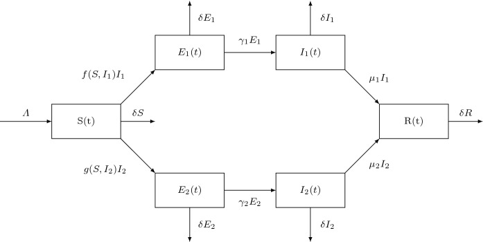
The properties $(H_1)$, $(H_2)$ and $(H_3)$, for the both functions f and g, are easily verified by several classical biological incidence rates such as the bilinear incidence function $\beta S$  [1, 15, 16], the saturated incidence function ${\displaystyle \frac{\beta S}{1+{\alpha }_{1}S}}$ or ${\displaystyle \frac{\beta S}{1+{\alpha }_{2}I}}$ [17, 18], Beddington–DeAngelis incidence function ${\displaystyle \frac{\beta S}{1+{\alpha }_{1}S+{\alpha }_{2}I}}$ [19–21], Crowley–Martin incidence function ${\displaystyle \frac{\beta S}{1+{\alpha }_{1}S+{\alpha }_{2}I+{\alpha }_1{\alpha }_{2}SI}}$ [22–24], the specific nonlinear incidence function ${\displaystyle \frac{\beta S}{1+{\alpha }_{1}S+{\alpha }_{2}I+{\alpha }_{3}SI}}$ [25–29] and non-monotone incidence function ${\displaystyle \frac{\beta S}{1+\alpha I^2}}$ [30–34]. The flowchart of the two-strain epidemiological SEIR model is illustrated in Fig. 1. Our main contribution centres around the global stability of multi-strain SEIR epidemic model with general incidence rates. In addition, a numerical comparison between our two-strain epidemic model results and COVID-19 clinical data will be conducted. It will be worthy to notice that the dynamics of SEIR COVID-19 epidemic model with two bilinear incidence functions was tackled in [35], and the authors introduce seasonality and stochasticity in order to describe the infection rate parameters. Taking into account non-monotone incidence function, the technique of sliding mode control was used to study an SEIR epidemic model describing COVID-19 disease [36]. The COVID-19 SEIR epidemiological model with Crowley–Martin incidence rate was studied [37], and the authors study the effect of different parameters on the disease spread. In our numerical comparison with COVID-19 clinical data, we will take into account the three latter incidence functions along with Beddington–DeAngelis incidence rate. A brief analysis to a more complex compartmental epidemic model will be established in Appendix of this paper.

Fig. 1.

Flowchart of two-strain SEIR model

The rest of this paper is outlined as follows. In the next section, we will establish the wellposedness of the suggested model by proving the existence, positivity and boundedness of solutions. In Sect. 3, we present an analysis of the model, we calculate the basic reproduction number of our epidemic model and we prove the global stability of the equilibria. Numerical simulations are given in Sect. 4 by using different specific incidence functions, and the comparison between the numerical results and COVID-19 clinical data is conducted in the same section. The generalization of the problem to a more complex compartmental model as well as concluding remarks is given at the end of this paper.

The problem wellposedness and steady states

Positivity and boundedness of solutions

For the problems dealing with population dynamics, all the variables must be positive and bounded. We will assume first that all the model parameters are positive.

Proposition 1

For all non-negative initial data, the solutions of the problem (1.1) exist, remain bounded and non-negative.

Moreover, we have $N(t)\le \frac{\Lambda }{\delta }+N(0)$.

Proof

By the fundamental theory of differential equations functional framework (see for instance [38] and the references therein), we confirm that there exists a unique local solution to the problem (1.1).

In order to prove the positivity result, we will show that any solution starting from non-negative orthant ${\mathbb{R}}_{+}^6=\{(S,E_1,E_2,I_1,I_2,R)\in {\mathbb{R}}^6:S\ge 0,E_1\ge 0,E_2\ge 0,I_1\ge 0,I_2\ge 0,R\ge 0\}$ remains there forever.

First, let

$$\begin{array}{cc}\hfill T=& {\displaystyle \text{sup}\{\tau \ge 0|\forall t\in [0,\tau ]\text{such that}S(t)\ge 0,}\hfill \\ \hfill & E_1(t)\ge 0,E_2(t)\ge 0,I_1(t)\ge 0,\hfill \\ \hfill & I_2(t)\ge 0,R(t)\ge 0\}\hfill \end{array}$$ 2.1

Let us now prove that $T=+\infty$. Suppose that T is finite; by continuity of solutions, we have

$$\begin{array}{cc}& S(T)=0\text{or}{E}_1(T)=0\text{or}{E}_2(T)=0\text{or}\hfill \\ \hfill & I_1(T)=0\text{or}{I}_2(T)=0\text{or}R(T)=0.\hfill \end{array}$$

If $S(T)=0$ before the other variables $E_1$, $E_2$, $I_1$, $I_2$, R, become zero. Therefore,

$$\begin{array}{c}\hfill {\displaystyle \frac{\mathrm{d}S(T)}{\mathrm{d}t}=\underset{t\to T^{-}}{lim}\frac{S(T)-S(t)}{T-t}=\underset{t\to T^{-}}{lim}\frac{-S(t)}{T-t}\le 0.}\\ \hfill \end{array}$$ 2.2

From the first equation of system (1.1), we have

$$\begin{array}{cc}\hfill \dot{S}(T)=& \Lambda -f(S(T),I_1(T))I_1(T)\hfill \\ \hfill & -g(S(T),I_2(T))I_2(T)-\delta S(T),\hfill \end{array}$$ 2.3

then,

$$\begin{array}{c}\hfill \dot{S}(T)=\Lambda -f(0,I_1(T))I_1(T)-g(0,I_2(T))I_2(T),\\ \hfill \end{array}$$ 2.4

However, from $(H_1)$ we have

$$\begin{array}{c}\hfill \dot{S}(T)=\Lambda >0\end{array}$$ 2.5

which presents a contradiction.

If $E_1(T)=0$ before S, $E_2$, $I_1$, $I_2$ and R. Then,

$$\begin{array}{c}\hfill {\displaystyle \frac{\mathrm{d}{E}_1(T)}{\mathrm{d}t}=\underset{t\to T^{-}}{lim}\frac{E_1(T)-E_1(t)}{T-t}=\underset{t\to T^{-}}{lim}\frac{-E_1(t)}{T-t}\le 0.}\\ \hfill \end{array}$$ 2.6

Again, from the second equation of the system (1.1) with the fact $E_1(T)=0$, we will have

$$\begin{array}{c}\hfill {\displaystyle \frac{\mathrm{d}{E}_1(T)}{\mathrm{d}t}=f(S,I_1)I_1.}\end{array}$$ 2.7

However, from $(H_1)$ and $(H_2)$, $f(S,I_1)I_1$ is positive, then we will have

$$\begin{array}{c}\hfill {\displaystyle \frac{\mathrm{d}{E}_1(T)}{\mathrm{d}t}>0.}\end{array}$$ 2.8

Also, if $I_1=0$ before S, $E_1$, $E_2$, $I_2$, R become zero then

$$\begin{array}{c}\hfill {\displaystyle \frac{\mathrm{d}{I}_1(T)}{\mathrm{d}t}=\underset{t\to T^{-}}{lim}\frac{I_1(T)-I_1(t)}{T-t}=\underset{t\to T^{-}}{lim}\frac{-I_1(t)}{T-t}\le 0.}\\ \hfill \end{array}$$ 2.9

But from the fourth equation of the system (1.1) with $I_1(T)=0$, we will have

$$\begin{array}{c}\hfill {\displaystyle \frac{\mathrm{d}{I}_1(T)}{\mathrm{d}t}={\gamma }_1{E}_1.}\end{array}$$ 2.10

Since ${\gamma }_1>0$, we have

$$\begin{array}{c}\hfill {\displaystyle \frac{\mathrm{d}{I}_1(T)}{\mathrm{d}t}={\gamma }_1{E}_1>0.}\end{array}$$ 2.11

This leads to contradiction.

Similar proofs for $E_2(t)$, $I_2(t)$ and R(t).

We conclude that T could not be finite, which implies that $S(t)\ge 0,E_1(t)\ge 0,E_2(t)\ge 0,I_1(t)\ge 0,I_2(t)\ge 0,R(t)\ge 0$ for all positive times. This proves the positivity of solutions.

About boundedness, let the total population

$$\begin{array}{c}\hfill N(t)=S(t)+E_1(t)+E_2(t)+I_1(t)+I_2(t)+R(t).\\ \hfill \end{array}$$ 2.12

From the system (1.1), we have

$$\begin{array}{c}\hfill {\displaystyle \frac{\mathrm{d}N(t)}{\mathrm{d}t}=\Lambda -\delta N(t),}\end{array}$$ 2.13

and therefore,

$$\begin{array}{c}\hfill {\displaystyle N(t)=\frac{\Lambda }{\delta }+K{\mathrm{e}}^{-\delta t},}\end{array}$$ 2.14

at $t=0$, we have

$$\begin{array}{c}\hfill {\displaystyle N(0)=\frac{\Lambda }{\delta }+K,}\end{array}$$ 2.15

then

$$\begin{array}{c}\hfill {\displaystyle N(t)=\frac{\Lambda }{\delta }+(N(0)-\frac{\Lambda }{\delta }){\mathrm{e}}^{-\delta t},}\end{array}$$ 2.16

consequently

$$\begin{array}{c}\hfill {\displaystyle N(t)\le \frac{\Lambda }{\delta }+N(0){\mathrm{e}}^{-\delta t},}\end{array}$$ 2.17

since $0<{\mathrm{e}}^{-\delta t}\le 1$, for all $t\ge 0$, we conclude that

$$\begin{array}{c}\hfill {\displaystyle N(t)\le \frac{\Lambda }{\delta }+N(0).}\end{array}$$ 2.18

This implies that N(t) is bounded, and so are $S(t),E_1(t),E_2(t),I_1(t),I_2(t)\text{and}R(t).$ Thus, the local solution can be prolonged to any positive time, which means that the unique solution exists globally. $\square$

The steady states

In this subsection, we show that there exist a disease-free equilibrium and three endemic equilibria. First, since the first five equations of the system (1.1) are independent of R and knowing that the number of the total population verifies the Eq. (2.14), so we can omit the sixth equation of the system (1.1). Therefore, the problem can be reduced to:

$$\begin{array}{c}\hfill \left\{\begin{array}{cc}& \frac{\mathrm{d}S}{\mathrm{d}t}=\Lambda -f(S,I_1)I_1-g(S,I_2)I_2-\delta S,\hfill \\ \hfill & \frac{\mathrm{d}{E}_1}{\mathrm{d}t}=f(S,I_1)I_1-({\gamma }_1+\delta )E_1,\hfill \\ \hfill & \frac{\mathrm{d}{E}_2}{\mathrm{d}t}=g(S,I_2)I_2-({\gamma }_2+\delta )E_2,\hfill \\ \hfill & \frac{\mathrm{d}{I}_1}{\mathrm{d}t}={\gamma }_1{E}_1-({\mu }_1+\delta )I_1,\hfill \\ \hfill & \frac{\mathrm{d}{I}_2}{\mathrm{d}t}={\gamma }_2{E}_2-({\mu }_2+\delta )I_2,\hfill \\ \hfill \end{array}\right)\end{array}$$ 2.19

with

$$\begin{array}{c}\hfill R=N-S-E_1-E_2-I_1-I_2.\end{array}$$ 2.20

As usual, the basic reproduction number can be defined as the average number of new cases of an infection caused by one infected individual when all the population individuals are susceptibles. We will use the next generation matrix $F{V}^{-1}$ to calculate the basic reproduction number $R_0$. The formula that gives us the basic reproduction number is: $R_0=\rho (F{V}^{-1}),$ where $\rho$ stands for the spectral radius, F is the non-negative matrix of new infection cases and V is the matrix of the transition of infections associated with the model (2.19). We have

$$\begin{array}{cc}\hfill F& =\left(\begin{array}{cccc}0& 0& f(\frac{\Lambda }{\delta },0)& 0\\ 0& 0& 0& g(\frac{\Lambda }{\delta },0)\\ 0& 0& 0& 0\\ 0& 0& 0& 0\end{array}\right),\hfill \\ \hfill V& =\left(\begin{array}{cccc}{\gamma }_1+\delta & 0& 0& 0\\ 0& {\gamma }_2+\delta & 0& 0\\ -{\gamma }_1& 0& {\mu }_1+\delta & 0\\ 0& -{\gamma }_2& 0& {\mu }_2+\delta \end{array}\right).\hfill \end{array}$$

So,

$$\begin{array}{c}\hfill F{V}^{-1}=\left(\begin{array}{cccc}{\displaystyle \frac{f(\frac{\Lambda }{\delta },0){\gamma }_1}{({\gamma }_1+\delta )({\mu }_1+\delta )}}& 0& {\displaystyle \frac{f(\frac{\Lambda }{\delta },0)}{({\mu }_1+\delta )}}& 0\\ 0& {\displaystyle \frac{g(\frac{\Lambda }{\delta },0){\gamma }_2}{({\gamma }_2+\delta )({\mu }_2+\delta )}}& 0& {\displaystyle \frac{g(\frac{\Lambda }{\delta },0)}{({\mu }_1+\delta )}}\\ 0& 0& 0& 0\\ 0& 0& 0& 0\end{array}\right).\end{array}$$

The basic reproduction number is the spectral radius of the matrix $F{V}^{-1}$. This fact implies that

$$\begin{array}{c}\hfill R_0=max\{R_0^1,R_0^2\},\end{array}$$ 2.21

with

$$\begin{array}{c}\hfill {\displaystyle R_0^1=\frac{f(\frac{\Lambda }{\delta },0){\gamma }_1}{({\gamma }_1+\delta )({\mu }_1+\delta )}}\end{array}$$ 2.22

and

$$\begin{array}{c}\hfill {\displaystyle R_0^2=\frac{g(\frac{\Lambda }{\delta },0){\gamma }_2}{({\gamma }_2+\delta )({\mu }_2+\delta )}.}\end{array}$$ 2.23

We denote

$$\begin{array}{c}\hfill a={\gamma }_1+\delta ,b={\gamma }_2+\delta ,c={\mu }_1+\delta ,e={\mu }_2+\delta ,\end{array}$$

then

$$\begin{array}{c}\hfill {\displaystyle R_0^1=\frac{f(\frac{\Lambda }{\delta },0){\gamma }_1}{\mathit{ac}}}\end{array}$$ 2.24

and

$$\begin{array}{c}\hfill {\displaystyle R_0^2=\frac{g(\frac{\Lambda }{\delta },0){\gamma }_2}{\mathit{be}}.}\end{array}$$ 2.25

We call $R_0^1$ the strain 1 reproduction number and $R_0^2$ the strain 2 reproduction number.

Theorem 1

The problem (2.19) have the disease-free equilibrium $E_f$ and three endemic equilibria ${\mathcal{E}}_{s_1}$, ${\mathcal{E}}_{s_2}$ and ${\mathcal{E}}_{s_t}$. Moreover, we have

• The strain 1 endemic equilibrium ${\mathcal{E}}_{s_1}$ exists when $R_0^1>1$.

• The strain 2 endemic equilibrium ${\mathcal{E}}_{s_2}$ exists when $R_0^2>1$.

• The third endemic equilibrium ${\mathcal{E}}_{s_t}$ exists when $R_0^1>1$ and $R_0^1>1$.

Proof

In order to find the steady states of the system (2.19), we solve the following equations

$$\begin{array}{cc}& \Lambda -f(S,I_1)I_1-g(S,I_2)I_2-\delta S=0,\hfill \end{array}$$ 2.26

$$\begin{array}{cc}& f(S,I_1)I_1-({\gamma }_1+\delta )E_1=0,\hfill \end{array}$$ 2.27

$$\begin{array}{cc}& g(S,I_2)I_2-({\gamma }_2+\delta )E_2=0,\hfill \end{array}$$ 2.28

$$\begin{array}{cc}& {\gamma }_1{E}_1-({\mu }_1+\delta )I_1=0,\hfill \end{array}$$ 2.29

$$\begin{array}{cc}& {\gamma }_2{E}_2-({\mu }_2+\delta )I_2=0.\hfill \end{array}$$ 2.30

From where, we obtain

• When $I_1=0\text{and}{I}_2=0$, we find the disease-free equilibrium

  $$\begin{array}{c}\hfill {\mathcal{E}}_f=\left({\displaystyle \frac{\Lambda }{\delta },0,0,0,0}\right).\end{array}$$
• When $I_1\ne 0\text{and}{I}_2=0$, we find the strain 1 endemic equilibrium defined as follows

  $$\begin{array}{cc}& {\mathcal{E}}_{s_1}=\left(S_1^{\ast },,,\frac{1}{a},(\Lambda -\delta S_1^{\ast }),,,0,,,\frac{{\gamma }_1}{\mathit{ac}},(\Lambda -\delta S_1^{\ast }),,,0\right),\hfill \\ \hfill & \text{where}{S}_1^{\ast }\in \left[{\displaystyle 0,\frac{\Lambda }{\delta }}\right].\hfill \end{array}$$

  Define now a function $\Psi \text{on}[0,+\infty [$ as follows

  $$\begin{array}{c}\hfill {\displaystyle \Psi (S)=f(S,\frac{{\gamma }_1}{\mathit{ac}}(\Lambda -\delta S))-\frac{\mathit{ac}}{{\gamma }_1}.}\end{array}$$ 2.31

  We have

  $$\begin{array}{c}\hfill {\displaystyle \frac{\partial \Psi (S)}{\partial S}=\frac{\partial f(S,I_1)}{\partial S}+\frac{\partial f(S,I_1)}{\partial I_1}\left({\displaystyle \frac{-\delta {\gamma }_1}{\mathit{ac}}}\right),}\\ \hfill \end{array}$$ 2.32

  using the conditions $(H_2)$ and $(H_3)$, we deduce that

  $$\begin{array}{c}\hfill {\displaystyle \frac{\partial \Psi (S)}{\partial S}\ge 0.}\end{array}$$ 2.33

  However, ${\displaystyle \Psi (0)=f(0,I_{1,s_1}^{\ast })-\frac{\mathit{ac}}{{\gamma }_1}=-\frac{\mathit{ac}}{{\gamma }_1}<0.}$ Therefore, for $R_0^1>1$, we he have

  $$\begin{array}{c}\hfill {\displaystyle \Psi \left(\frac{\Lambda }{\delta }\right)=f\left(\frac{\Lambda }{\delta },,,0\right)-\frac{\mathit{ac}}{{\gamma }_1}=\frac{\mathit{ac}}{{\gamma }_1}(R_0^1-1)>0.}\\ \hfill \end{array}$$ 2.34

  Hence, there exists a unique strain 1 endemic equilibrium

  $$\begin{array}{c}\hfill {\displaystyle {\mathcal{E}}_{s_1}=\left(S_1^{\ast },,,E_{1,s_1}^{\ast },,,E_{2,s_1}^{\ast },,,I_{1,s_1}^{\ast },,,I_{2,s_1}^{\ast }\right),}\end{array}$$ 2.35

  with ${\displaystyle S_1^{\ast }\in ]0,\frac{\Lambda }{\delta }[}$, $E_{1,s_1}^{\ast }>0$, $I_{1,s_1}^{\ast }>0$ and $E_{2,s_1}^{\ast }=I_{2,s_1}^{\ast }=0$.
• When $I_2\ne 0\text{and}{I}_1=0$, we find the strain 2 endemic equilibrium defined as follows

  $$\begin{array}{cc}& {\mathcal{E}}_{s_2}=\left(S_2^{\ast },,,0,,,\frac{1}{b},(\Lambda -\delta S_2^{\ast }),,,0,,,\frac{{\gamma }_2}{\mathit{be}},(\Lambda -\delta S_2^{\ast })\right),\hfill \\ \hfill & \text{where}{S}_2^{\ast }\in \left[{\displaystyle 0,\frac{\Lambda }{\delta }}\right].\hfill \end{array}$$

  Define also a function $\Phi \text{on}[0,+\infty [$ as follows

  $$\begin{array}{c}\hfill {\displaystyle \Phi (S)=g(S,\frac{{\gamma }_2}{\mathit{be}}(\Lambda -\delta S))-\frac{\mathit{be}}{{\gamma }_2}.}\end{array}$$ 2.36

  We have

  $$\begin{array}{c}\hfill {\displaystyle \frac{\partial \Phi (S)}{\partial S}=\frac{\partial g(S,I_2)}{\partial S}+\frac{\partial g(S,I_2)}{\partial I_2}\left({\displaystyle \frac{-\delta {\gamma }_2}{\mathit{be}}}\right),}\\ \hfill \end{array}$$ 2.37

  using the conditions $(H_2)$ and $(H_3)$, we conclude that

  $$\begin{array}{c}\hfill {\displaystyle \frac{\partial \Phi (S)}{\partial S}\ge 0.}\end{array}$$ 2.38

  However, ${\displaystyle \Phi (0)=g(0,I_{2,s_2}^{\ast })-\frac{\mathit{be}}{{\gamma }_2}=-\frac{\mathit{be}}{{\gamma }_2}<0}$. So, for $R_0^2>1$, we have

  $$\begin{array}{c}\hfill {\displaystyle \Phi \left(\frac{\Lambda }{\delta }\right)=g\left(\frac{\Lambda }{\delta },,,0\right)-\frac{\mathit{be}}{{\gamma }_2}=\frac{\mathit{be}}{{\gamma }_2}(R_0^2-1)>0.}\\ \hfill \end{array}$$ 2.39

  Hence, there exists a unique strain 2 endemic equilibrium

  $$\begin{array}{c}\hfill {\displaystyle {\mathcal{E}}_{s_2}=\left(S_2^{\ast },,,E_{1,s_2}^{\ast },,,E_{2,s_2}^{\ast },,,I_{1,s_2}^{\ast },,,I_{2,s_2}^{\ast }\right),}\end{array}$$ 2.40

  with $S_2^{\ast }\in \left]{\displaystyle 0,\frac{\Lambda }{\delta }}\right[$, $E_{2,s_2}^{\ast }>0$, $I_{2,s_2}^{\ast }>0$ and $E_{1,s_2}^{\ast }=I_{1,s_2}^{\ast }=0$.
• When $I_1\ne 0\text{and}{I}_2\ne 0$, we find the third endemic equilibrium defined as follows

  $$\begin{array}{c}\hfill {\displaystyle {\mathcal{E}}_t=\left(S_t^{\ast },,,E_{1,t}^{\ast },,,E_{2,t}^{\ast },,,I_{1,t}^{\ast },,,I_{2,t}^{\ast }\right),}\end{array}$$ 2.41

  where

  $$\begin{array}{cc}\hfill E_{1,t}^{\ast }=& {\displaystyle \frac{c}{{\gamma }_1}{I}_{1,t}^{\ast },E_{2,t}^{\ast }=\frac{e}{{\gamma }_2}{I}_{2,t}^{\ast },}\hfill \end{array}$$ 2.42

  $$\begin{array}{cc}\hfill S_t^{\ast }=& {\displaystyle \frac{1}{\delta }\left[{\displaystyle \Lambda -\frac{f(\frac{\Lambda }{\delta },0)}{R_0^1}{I}_{1,t}^{\ast }-\frac{g(\frac{\Lambda }{\delta },0)}{R_0^2}{I}_{2,t}^{\ast },}\right]}\hfill \\ \hfill \end{array}$$ 2.43

  with ${\displaystyle \Lambda \ge \frac{f(\frac{\Lambda }{\delta },0)}{R_0^1}{I}_{1,t}^{\ast }+\frac{g(\frac{\Lambda }{\delta },0)}{R_0^2}{I}_{2,t}^{\ast }}$, $R_0^1>1$ and $R_0^2>1$. $\square$

Global stability of equilibria

Global stability of disease-free equilibrium

Theorem 2

If $R_0\le 1$, then the disease-free equilibrium ${\mathcal{E}}_f$ is globally asymptotically stable.

Proof

First, we consider the following Lyapunov function in ${\mathbb{R}}_{+}^5$:

$$\begin{array}{cc}\hfill {\mathcal{L}}_f(S,E_1,E_2,I_1,I_2)=& S-S_0^{\ast }-{\int }_{S_0^{\ast }}^S\frac{f(S_0^{\ast },0)}{f(X,0)}\mathrm{d}X\hfill \\ \hfill & +E_1+E_2+\frac{a}{{\gamma }_1}{I}_1+\frac{b}{{\gamma }_2}{I}_2.\hfill \\ \hfill \end{array}$$ 3.1

The time derivative is given by

$$\begin{array}{cc}\hfill {\dot{\mathcal{L}}}_f(S,E_1,E_2,I_1,I_2)& =\dot{S}-\frac{f(S_0^{\ast },0)}{f(S,0)}\dot{S}+\dot{E_1}+\dot{E_2}\hfill \\ \hfill & +\frac{a}{{\gamma }_1}\dot{I_1}+\frac{b}{{\gamma }_2}\dot{I_2},\hfill \\ \hfill & =\delta S_0^{\ast }\left(1,-,\frac{S}{S_0^{\ast }}\right)\left(1,-,\frac{f(S_0^{\ast },0)}{f(S,0)}\right)\hfill \\ \hfill & +\frac{\mathit{ac}}{{\gamma }_1}{I}_1\left(\frac{f(S,I_1)}{f(S,0)},R_0^1,-,1\right)\hfill \end{array}$$ 3.2

$$\begin{array}{cc}& +\frac{\mathit{be}}{{\gamma }_2}{I}_2\left(\frac{f(S_0^{\ast },0)}{f(S,0)},\frac{g(S,I_2)}{g(S_0^{\ast },0)},R_0^2,-,1\right)\hfill \end{array}$$ 3.3

$$\begin{array}{cc}& \le \delta S_0^{\ast }\left(1,-,\frac{S}{S_0^{\ast }}\right)\left(1,-,\frac{f(S_0^{\ast },0)}{f(S,0)}\right)\hfill \\ \hfill & +\frac{\mathit{ac}}{{\gamma }_1}{I}_1\left(R_0^1,-,1\right)\hfill \\ \hfill & +\frac{\mathit{be}}{{\gamma }_2}{I}_2\left({\displaystyle \frac{f(S_0^{\ast },0)}{f(S,0)}\frac{g(S,I_2)}{g(S_0^{\ast },0)}{R}_0^2-1}\right)\hfill \end{array}$$ 3.4

We will discuss two cases:

• If $S\le S_0^{\ast }$, using $(H_2),$ we will have ${\displaystyle \frac{g(S,I_2)}{g(S_0^{\ast },0)}\le 1}$, then,

  $$\begin{array}{cc}\hfill {\dot{\mathcal{L}}}_f(S,E_1,E_2,I_1,I_2)& \le \delta S_0^{\ast }\left(1,-,\frac{S}{S_0^{\ast }}\right)\left(1,-,\frac{f(S_0^{\ast },0)}{f(S,0)}\right)\hfill \\ \hfill & +\frac{\mathit{ac}}{{\gamma }_1}{I}_1\left(R_0^1,-,1\right)\hfill \\ \hfill & +\frac{\mathit{be}}{{\gamma }_2}{I}_2\left({\displaystyle \frac{f(S_0^{\ast },0)}{f(S,0)}{R}_0^2-1}\right).\hfill \end{array}$$ 3.5

  Since ${\displaystyle R_0^2\le \frac{f(S,0)}{f(S_0^{\ast },0)}\le 1}$, we obtain

  $$\begin{array}{c}\hfill {\displaystyle \frac{f(S_0^{\ast },0)}{f(S,0)}{R}_0^2-1\le 0.}\end{array}$$ 3.6

  Otherwise, ${\displaystyle 1-\frac{f(S_0^{\ast },0)}{f(S,0)}\le 0,}$ therefore

  $$\begin{array}{c}\hfill \delta S_0^{\ast }\left({\displaystyle 1-\frac{S}{S_0^{\ast }}}\right)\left({\displaystyle 1-\frac{f(S_0^{\ast },0)}{f(S,0)}}\right)\le 0.\end{array}$$ 3.7
• If $S_0^{\ast }<S$, using $(H_2),$ we will have ${\displaystyle \frac{g(S,I_2)}{g(S_0^{\ast },0)}>1}$ and ${\displaystyle \frac{f(S_0^{\ast },0)}{f(S,0)}<1}$ then,

  $$\begin{array}{cc}\hfill {\dot{\mathcal{L}}}_f(S,E_1,E_2,I_1,I_2)& \le \delta S_0^{\ast }\left(1,-,\frac{S}{S_0^{\ast }}\right)\left(1,-,\frac{f(S_0^{\ast },0)}{f(S,0)}\right)\hfill \\ \hfill & +\frac{\mathit{ac}}{{\gamma }_1}{I}_1\left(R_0^1,-,1\right)\hfill \\ \hfill & +\frac{\mathit{be}}{{\gamma }_2}{I}_2\left({\displaystyle \frac{g(S,I_2)}{g(S_0^{\ast },0)}{R}_0^2-1}\right).\hfill \end{array}$$ 3.8

  Since ${\displaystyle R_0^2<\frac{g(S_0^{\ast },0)}{g(S,I_2)}<1}$, we obtain

  $$\begin{array}{c}\hfill {\displaystyle \frac{g(S,I_2)}{g(S_0^{\ast },0)}{R}_0^2-1<0.}\end{array}$$ 3.9

  From ${\displaystyle \frac{f(S_0^{\ast },0)}{f(S,0)}<1}$, we have

  $$\begin{array}{c}\hfill \delta S_0^{\ast }\left({\displaystyle 1-\frac{S}{S_0^{\ast }}}\right)\left({\displaystyle 1-\frac{f(S_0^{\ast },0)}{f(S,0)}}\right)\le 0.\end{array}$$ 3.10

By the above discussion, we deduce that, if $R_0^2\le 1$ and $R_0^1\le 1$ (which means that $R_0\le 1$), then

$$\begin{array}{c}\hfill {\dot{\mathcal{L}}}_f(S,E_1,E_2,I_1,I_2)\le 0.\end{array}$$ 3.11

Thus, the disease-free equilibrium point ${\mathcal{E}}_f$ is globally asymptotically stable when $R_0\le 1$. $\square$

Global stability of strain 1 endemic equilibrium

For the global stability of ${\mathcal{E}}_{s_1}$, we assume that the function f satisfies the following condition:

$$\begin{array}{cc}& \left(1,-,\frac{f(S,I_1)}{f(S,I_{1,s_1}^{\ast })}\right)\left(\frac{f(S,I_{1,s_1}^{\ast })}{f(S,I_1)},-,\frac{I_1}{I_{1,s_1}^{\ast }}\right)\le 0,\hfill \\ \hfill & \forall S,I_1>0.\hfill \\ \hfill \end{array}$$ 3.12

Theorem 3

The strain 1 endemic equilibrium ${\mathcal{E}}_{s_1}$ is globally asymptotically stable when $R_0^2\le 1<R_0^1$.

Proof

First, we consider the Lyapunov function ${\mathcal{L}}_1$ defined by:

$$\begin{array}{cc}& {\mathcal{L}}_1(S,E_1,E_2,I_1,I_2)=S-S_1^{\ast }-{\int }_{S_1^{\ast }}^S\frac{f(S_1^{\ast },I_{1,s_1}^{\ast })}{f(X,I_{1,s_1}^{\ast })}\mathrm{d}X+E_1^{\ast }\left(\frac{E_1}{E_{1,s_1}^{\ast }},-,ln,\left(\frac{E_1}{E_{1,s_1}^{\ast }}\right),-,1\right)\hfill \\ \hfill & +E_2+\frac{a}{{\gamma }_1}{I}_{1,s_1}^{\ast }\left(\frac{I_1}{I_{1,s_1}^{\ast }},-,ln,\left(\frac{I_1}{I_{1,s_1}^{\ast }}\right),-,1\right)+\frac{b}{{\gamma }_2}{I}_2.\hfill \end{array}$$ 3.13

The time derivative is given by

$$\begin{array}{cc}\hfill {\dot{\mathcal{L}}}_1(S,E_1,E_2,I_1,I_2)=& \left(\Lambda ,-,f,(S,I_1),I_1,-,g,(S,I_2),I_2,-,\delta ,S\right)\hfill \\ \hfill & {\displaystyle \left(1,-,\frac{f(S_1^{\ast },I_{1,s_1}^{\ast })}{f(S,I_{1,s_1}^{\ast })}\right)}\hfill \\ \hfill & {\displaystyle +\left(f,(S,I_1),I_1,-,a,E_1\right)\left(1,-,\frac{E_{1,s_1}^{\ast }}{E_1}\right)}\hfill \\ \hfill & {\displaystyle +\left(g,(S,I_2),I_2,-,b,E_2\right)}\hfill \\ \hfill & {\displaystyle +\frac{a}{{\gamma }_1}\left({\gamma }_1,E_1,-,c,I_1\right)\left(1,-,\frac{I_{1,s_1}^{\ast }}{I_1}\right)}\hfill \\ \hfill & {\displaystyle +\frac{b}{{\gamma }_2}\left({\gamma }_2,E_2,-,e,I_2\right).}\hfill \end{array}$$ 3.14

We have

$$\begin{array}{c}\hfill \left\{\begin{array}{cc}& \Lambda =\delta S_1^{\ast }+f(S_1^{\ast },I_{1,s_1}^{\ast })I_{1,s_1}^{\ast },\hfill \\ \hfill & {\displaystyle f(S_1^{\ast },I_{1,s_1}^{\ast })I_{1,s_1}^{\ast }=\frac{\mathit{ac}}{{\gamma }_1}{I}_{1,s_1}^{\ast }=a{E}_{1,s_1}^{\ast },}\hfill \\ \hfill & {\displaystyle \frac{E_{1,s_1}^{\ast }}{I_{1,s_1}^{\ast }}=\frac{c}{{\gamma }_1}.}\hfill \end{array}\right)\end{array}$$ 3.15

Therefore,

$$\begin{array}{cc}\hfill {\dot{\mathcal{L}}}_1(S,E_1,E_2,I_1,I_2)=& {\displaystyle \delta S_1^{\ast }\left(1,-,\frac{f(S_1^{\ast },I_{1,s_1}^{\ast })}{f(S,I_{1,s_1}^{\ast })}\right)}\hfill \\ \hfill & {\displaystyle -\delta S\left(1,-,\frac{f(S_1^{\ast },I_{1,s_1}^{\ast })}{f(S,I_{1,s_1}^{\ast })}\right)}\hfill \\ \hfill & +f(S_1^{\ast },I_{1,s_1}^{\ast })I_{1,s_1}^{\ast }\hfill \\ \hfill & -f(S_1^{\ast },I_{1,s_1}^{\ast })I_{1,s_1}^{\ast }\frac{f(S_1^{\ast },I_{1,s_1}^{\ast })}{f(S,I_{1,s_1}^{\ast })}\hfill \\ \hfill & +\frac{f(S_1^{\ast },I_{1,s_1}^{\ast })}{f(S,I_{1,s_1}^{\ast })}f(S,I_1)I_1\hfill \\ \hfill & -f(S,I_1)\frac{I_1{E}_{1,s_1}^{\ast }}{E_1}+a{E}_{1,s_1}^{\ast }\hfill \\ \hfill & {\displaystyle -\frac{\mathit{ac}}{{\gamma }_1}{I}_1-\frac{a{I}_{1,s_1}^{\ast }}{I_1}{E}_1+\frac{\mathit{ac}}{{\gamma }_1}{I}_{1,s_1}^{\ast }}\hfill \\ \hfill & +\frac{f(S_1^{\ast },I_{1,s_1}^{\ast })}{f(S,I_{1,s_1}^{\ast })}g(S,I_2)I_2-\frac{\mathit{be}}{{\gamma }_2}{I}_2.\hfill \end{array}$$ 3.16

Then,

$$\begin{array}{cc}& {\dot{\mathcal{L}}}_1(S,E_1,E_2,I_1,I_2)=a{E}_{1,s_1}^{\ast }\left(4,-,\frac{a{E}_{1,s_1}^{\ast }}{f(S,I_{1,s_1}^{\ast })I_{1,s_1}^{\ast }},-,\frac{f(S,I_1)I_1}{a{E}_1},-,\frac{I_{1,s_1}^{\ast }{E}_1}{I_1{E}_{1,s_1}^{\ast }},-,\frac{f(S,I_{1,s_1}^{\ast })}{f(S,I_1)}\right)\hfill \\ \hfill & +a{E}_{1,s_1}^{\ast }\left(\frac{f(S,I_{1,s_1}^{\ast })}{f(S,I_1)},+,\frac{f(S,I_1)}{f(S,I_{1,s_1}^{\ast })},\frac{I_1}{I_{1,s_1}^{\ast }},-,\frac{I_1}{I_{1,s_1}^{\ast }},-,1\right)\hfill \\ \hfill & +\frac{f(S_1^{\ast },I_{1,s_1}^{\ast })}{f(S,I_{1,s_1}^{\ast })}g(S,I_2)I_2-\frac{\mathit{be}}{{\gamma }_2}{I}_2\hfill \end{array}$$ 3.17

$$\begin{array}{cc}& {\dot{\mathcal{L}}}_1(S,E_1,E_2,I_1,I_2)=a{E}_{1,s_1}^{\ast }\left(4,-,\frac{a{E}_{1,s_1}^{\ast }}{f(S,I_{1,s_1}^{\ast })I_{1,s_1}^{\ast }},-,\frac{f(S,I_1)I_1}{a{E}_1},-,\frac{I_{1,s_1}^{\ast }{E}_1}{I_1{E}_{1,s_1}^{\ast }},-,\frac{f(S,I_{1,s_1}^{\ast })}{f(S,I_1)}\right)\hfill \\ \hfill & +a{E}_{1,s_1}^{\ast }\left(\frac{f(S,I_{1,s_1}^{\ast })}{f(S,I_1)},+,\frac{f(S,I_1)}{f(S,I_{1,s_1}^{\ast })},\frac{I_1}{I_{1,s_1}^{\ast }},-,\frac{I_1}{I_{1,s_1}^{\ast }},-,1\right)\hfill \\ \hfill & +\frac{\mathit{be}}{{\gamma }_2}{I}_2\left({\displaystyle \frac{f(S_1^{\ast },I_{1,s_1}^{\ast })}{f(S,I_{1,s_1}^{\ast })}\frac{g(S,I_2)}{g(S_0^{\ast },0)}{R}_0^2-1}\right).\hfill \end{array}$$ 3.18

From $(H_2)$ and $(H_3)$, we have ${\displaystyle \frac{g(S,I_2)}{g(S_0^{\ast },0)}\le 1,}$ then,

$$\begin{array}{cc}& {\dot{\mathcal{L}}}_1(S,E_1,E_2,I_1,I_2)\le a{E}_{1,s_1}^{\ast }\left(4,-,\frac{a{E}_{1,s_1}^{\ast }}{f(S,I_{1,s_1}^{\ast })I_{1,s_1}^{\ast }},-,\frac{f(S,I_1)I_1}{a{E}_1},-,\frac{I_{1,s_1}^{\ast }{E}_1}{I_1{E}_{1,s_1}^{\ast }},-,\frac{f(S,I_{1,s_1}^{\ast })}{f(S,I_1)}\right)\hfill \\ \hfill & +a{E}_{1,s_1}^{\ast }\left(\frac{f(S,I_{1,s_1}^{\ast })}{f(S,I_1)},+,\frac{f(S,I_1)}{f(S,I_{1,s_1}^{\ast })},\frac{I_1}{I_{1,s_1}^{\ast }},-,\frac{I_1}{I_{1,s_1}^{\ast }},-,1\right)+\frac{\mathit{be}}{{\gamma }_2}{I}_2\left({\displaystyle \frac{f(S_1^{\ast },I_{1,s_1}^{\ast })}{f(S,I_{1,s_1}^{\ast })}{R}_0^2-1}\right),\hfill \end{array}$$ 3.19

From (3.12), we have

$$\begin{array}{cc}& \left(\frac{f(S,I_{1,s_1}^{\ast })}{f(S,I_1)},+,\frac{f(S,I_1)}{f(S,I_{1,s_1}^{\ast })},\frac{I_1}{I_{1,s_1}^{\ast }},-,\frac{I_1}{I_{1,s_1}^{\ast }},-,1\right)\hfill \\ \hfill & =\left(1,-,\frac{f(S,I_1)}{f(S,I_{1,s_1}^{\ast })}\right)\left(\frac{f(S,I_{1,s_1}^{\ast })}{f(S,I_1)},-,\frac{I_1}{I_{1,s_1}^{\ast }}\right)\le 0,\hfill \end{array}$$ 3.20

by the relation between arithmetic and geometric means, we have

$$\begin{array}{c}\hfill \left(4,-,\frac{a{E}_{1,s_1}^{\ast }}{f(S,I_{1,s_1}^{\ast })I_{1,s_1}^{\ast }},-,\frac{f(S,I_1)I_1}{a{E}_1},-,\frac{I_{1,s_1}^{\ast }{E}_1}{I_1{E}_{1,s_1}^{\ast }},-,\frac{f(S,I_{1,s_1}^{\ast })}{f(S,I_1)}\right)\le 0,\\ \hfill \end{array}$$ 3.21

We discuss two cases:

• If $S_1^{\ast }\le S$, from $(H_2)$, we will have ${\displaystyle \frac{f(S_1^{\ast },I_{1,s_1}^{\ast })}{f(S,I_{1,s_1}^{\ast })}\le 1,}$ since $\left({\displaystyle \frac{f(S_1^{\ast },I_{1,s_1}^{\ast })}{f(S,I_{1,s_1}^{\ast })}{R}_0^2-1}\right)\le 0$, we obtain, for $R_0^2\le 1,$ the following ${\dot{\mathcal{L}}}_1\le 0.$

• If $S\le S_1^{\ast },$ from $(H_2)$, we will have ${\displaystyle \frac{f(S_1^{\ast },I_{1,s_1}^{\ast })}{f(S,I_{1,s_1}^{\ast })}\ge 1,}$ since ${\displaystyle R_0^2\le \frac{f(S,I_{1,s_1}^{\ast })}{f(S_1^{\ast },I_{1,s_1}^{\ast })}\le 1,}$ we obtain ${\displaystyle \frac{f(S_1^{\ast },I_{1,s_1}^{\ast })}{f(S,I_{1,s_1}^{\ast })}{R}_0^2-1\le 0,}$ which implies, ${\dot{\mathcal{L}}}_1\le 0.$ By the above discussion, we deduce that if $R_0^2\le 1,$ we will have ${\dot{\mathcal{L}}}_1\le 0.$

We conclude that the steady state ${\mathcal{E}}_{s_1}$ is globally asymptotically stable when $R_0^2\le 1$ and $1<R_0^1$. $\square$

Global stability of strain 2 endemic equilibrium

For the global stability of ${\mathcal{E}}_{s_2}$, we assume that the function g satisfies the following condition:

$$\begin{array}{c}\hfill \left(1,-,\frac{g(S,I_2)}{g(S,I_{2,s_2}^{\ast })}\right)\left(\frac{g(S,I_{2,s_2}^{\ast })}{g(S,I_2)},-,\frac{I_2}{I_{2,s_2}^{\ast }}\right)\le 0,\forall S,I_2>0.\\ \hfill \end{array}$$ 3.22

Theorem 4

The strain 2 endemic equilibrium point ${\mathcal{E}}_{s_2}$ is globally asymptotically stable when $R_0^1\le 1<R_0^2$.

Proof

First, we consider the Lyapunov function ${\mathcal{L}}_2$ defined by:

$$\begin{array}{cc}\hfill {\mathcal{L}}_2(S,E_1,E_2,I_1,I_2)=& S-S_2^{\ast }-{\int }_{S_2^{\ast }}^S\frac{g(S_2^{\ast },I_{2,s_2}^{\ast })}{g(X,I_{2,s_2}^{\ast })}\mathrm{d}X\hfill \\ \hfill & +E_{2,s_2}^{\ast }\left(\frac{E_2}{E_{2,s_2}^{\ast }},-,ln,\left(\frac{E_2}{E_{2,s_2}^{\ast }}\right),-,1\right)\hfill \\ \hfill & +E_1+\frac{a}{{\gamma }_1}{I}_1\hfill \\ \hfill & {\displaystyle +\frac{b}{{\gamma }_2}{I}_{2,s_2}^{\ast }\left(\frac{I_2}{I_{2,s_2}^{\ast }},-,ln,\left(\frac{I_2}{I_{2,s_2}^{\ast }}\right),-,1\right).}\hfill \end{array}$$ 3.23

The time derivative is given by

$$\begin{array}{cc}\hfill {\dot{\mathcal{L}}}_2(S,E_1,E_2,I_1,I_2)=& \left(\Lambda ,-,f,(S,I_1),I_1,-,g,(S,I_2),I_2,-,\delta ,S\right)\hfill \\ \hfill & {\displaystyle \left(1,-,\frac{g(S_2^{\ast },I_{2,s_2}^{\ast })}{g(S,I_{2,s_2}^{\ast })}\right)}\hfill \\ \hfill & {\displaystyle +\left(g,(S,I_2),I_2,-,b,E_2\right)\left(1,-,\frac{E_{2,s_2}^{\ast }}{E_2}\right)}\hfill \\ \hfill & {\displaystyle +\left(f,(S,I_1),I_1,-,a,E_1\right)}\hfill \\ \hfill & {\displaystyle +\frac{b}{{\gamma }_2}\left({\gamma }_2,E_2,-,e,I_2\right)\left(1,-,\frac{I_{2,s_2}^{\ast }}{I_2}\right)}\hfill \\ \hfill & {\displaystyle +\frac{a}{{\gamma }_1}\left({\gamma }_1,E_1,-,c,I_1\right).}\hfill \end{array}$$ 3.24

We have

$$\begin{array}{c}\hfill \left\{\begin{array}{cc}& \Lambda =\delta S_2^{\ast }+g(S_2^{\ast },I_{2,s_2}^{\ast })I_{2,s_2}^{\ast },\hfill \\ \hfill & {\displaystyle g(S_2^{\ast },I_{2,s_2}^{\ast })I_{2,s_2}^{\ast }=\frac{\mathit{be}}{{\gamma }_2}{I}_{2,s_2}^{\ast }=b{E}_{2,s_2}^{\ast },}\hfill \\ \hfill & {\displaystyle \frac{E_{2,s_2}^{\ast }}{I_{2,s_2}^{\ast }}=\frac{e}{{\gamma }_2}.}\hfill \end{array}\right)\end{array}$$ 3.25

Therefore,

$$\begin{array}{cc}\hfill {\dot{\mathcal{L}}}_2(S,E_1,E_2,I_1,I_2)=& {\displaystyle \delta S_2^{\ast }\left(1,-,\frac{g(S_2^{\ast },I_{2,s_2}^{\ast })}{g(S,I_{2,s_2}^{\ast })}\right)}\hfill \\ \hfill & {\displaystyle -\delta S\left(1,-,\frac{g(S_2^{\ast },I_{2,s_2}^{\ast })}{g(S,I_{2,s_2}^{\ast })}\right)}\hfill \\ \hfill & +g(S_2^{\ast },I_{2,s_2}^{\ast })I_{2,s_2}^{\ast }\hfill \\ \hfill & -g(S_2^{\ast },I_{2,s_2}^{\ast })I_{2,s_2}^{\ast }\frac{g(S_2^{\ast },I_{2,s_2}^{\ast })}{g(S,I_{2,s_2}^{\ast })}\hfill \\ \hfill & +\frac{g(S_2^{\ast },I_{2,s_2}^{\ast })}{g(S,I_{2,s_2}^{\ast })}g(S,I_2)I_2\hfill \\ \hfill & {\displaystyle -g(S,I_2)\frac{I_2{E}_{2,s_2}^{\ast }}{E_2}+b{E}_{2,s_2}^{\ast }-\frac{\mathit{be}}{{\gamma }_2}{I}_2}\hfill \\ \hfill & {\displaystyle -\frac{b{I}_{2,s_2}^{\ast }}{I_2}{E}_2+\frac{\mathit{be}}{{\gamma }_2}{I}_{2,s_2}^{\ast }}\hfill \\ \hfill & +\frac{g(S_2^{\ast },I_{2,s_2}^{\ast })}{g(S,I_{2,s_2}^{\ast })}f(S,I_1)I_1-\frac{\mathit{ac}}{{\gamma }_1}{I}_1,\hfill \end{array}$$ 3.26

then

$$\begin{array}{cc}& {\dot{\mathcal{L}}}_2(S,E_1,E_2,I_1,I_2)=b{E}_{2,s_2}^{\ast }\left(4,-,\frac{b{E}_{2,s_2}^{\ast }}{g(S,I_{2,s_2}^{\ast })I_{2,s_2}^{\ast }},-,\frac{g(S,I_2)I_2}{b{E}_2},-,\frac{I_{2,s_2}^{\ast }{E}_2}{I_2{E}_{2,s_2}^{\ast }},-,\frac{g(S,I_{2,s_2}^{\ast })}{g(S,I_2)}\right)\hfill \\ \hfill & +b{E}_{2,s_2}^{\ast }\left(\frac{g(S,I_{2,s_2}^{\ast })}{g(S,I_2)},+,\frac{g(S,I_2)}{g(S,I_{2,s_2}^{\ast })},\frac{I_2}{I_{2,s_2}^{\ast }},-,\frac{I_2}{I_{2,s_2}^{\ast }},-,1\right)+\frac{g(S_2^{\ast },I_{2,s_2}^{\ast })}{g(S,I_{12,s_2}^{\ast })}f(S,I_1)I_1-\frac{\mathit{ac}}{{\gamma }_1}{I}_1\hfill \end{array}$$ 3.27

$$\begin{array}{cc}& {\dot{\mathcal{L}}}_2(S,E_1,E_2,I_1,I_2)=b{E}_{2,s_2}^{\ast }\left(4,-,\frac{b{E}_{2,s_2}^{\ast }}{g(S,I_{2,s_2}^{\ast })I_{2,s_2}^{\ast }},-,\frac{g(S,I_2)I_2}{b{E}_2},-,\frac{I_{2,s_2}^{\ast }{E}_2}{I_2{E}_{2,s_2}^{\ast }},-,\frac{g(S,I_{2,s_2}^{\ast })}{g(S,I_2)}\right)\hfill \\ \hfill & +b{E}_{2,s_2}^{\ast }\left(\frac{g(S,I_{2,s_2}^{\ast })}{g(S,I_2)},+,\frac{g(S,I_2)}{g(S,I_{2,s_2}^{\ast })},\frac{I_2}{I_{2,s_2}^{\ast }},-,\frac{I_2}{I_{2,s_2}^{\ast }},-,1\right)\hfill \\ \hfill & +\frac{\mathit{ac}}{{\gamma }_1}{I}_1\left({\displaystyle \frac{g(S_2^{\ast },I_{2,s_2}^{\ast })}{g(S,I_{2,s_2}^{\ast })}\frac{f(S,I_1)}{f(S_0^{\ast },0)}{R}_0^1-1}\right).\hfill \end{array}$$ 3.28

From $(H_2)$ and $(H_3)$, we have ${\displaystyle \frac{f(S,I_1)}{f(S_0^{\ast },0)}\le 1,}$ then,

$$\begin{array}{cc}& {\dot{\mathcal{L}}}_2(S,E_1,E_2,I_1,I_2)\le b{E}_{2,s_2}^{\ast }\left(4,-,\frac{b{E}_{2,s_2}^{\ast }}{g(S,I_{2,s_2}^{\ast })I_{2,s_2}^{\ast }},-,\frac{g(S,I_2)I_2}{b{E}_2},-,\frac{I_{2,s_2}^{\ast }{E}_2}{I_2{E}_{2,s_2}^{\ast }},-,\frac{g(S,I_{2,s_2}^{\ast })}{g(S,I_2)}\right)\hfill \\ \hfill & +b{E}_{2,s_2}^{\ast }\left(\frac{g(S,I_{2,s_2}^{\ast })}{g(S,I_2)},+,\frac{g(S,I_2)}{g(S,I_{2,s_2}^{\ast })},\frac{I_2}{I_{2,s_2}^{\ast }},-,\frac{I_2}{I_{2,s_2}^{\ast }},-,1\right)+\frac{\mathit{ac}}{{\gamma }_1}{I}_1\left({\displaystyle \frac{g(S_2^{\ast },I_{2,s_2}^{\ast })}{g(S,I_{2,s_2}^{\ast })}{R}_0^1-1}\right),\hfill \end{array}$$ 3.29

From (3.22), we have

$$\begin{array}{cc}& \left(\frac{g(S,I_{2,s_2}^{\ast })}{g(S,I_2)},+,\frac{g(S,I_2)}{g(S,I_{2,s_2}^{\ast })},\frac{I_2}{I_{2,s_2}^{\ast }},-,\frac{I_2}{I_{2,s_2}^{\ast }},-,1\right)\hfill \\ \hfill & =\left(1,-,\frac{g(S,I_2)}{g(S,I_{2,s_2}^{\ast })}\right)\left(\frac{g(S,I_{2,s_2}^{\ast })}{g(S,I_2)},-,\frac{I_2}{I_{2,s_2}^{\ast }}\right)\le 0.\hfill \end{array}$$ 3.30

By the relation between arithmetic and geometric means, we have

$$\begin{array}{c}\hfill \left(4,-,\frac{b{E}_{2,s_2}^{\ast }}{g(S,I_{2,s_2}^{\ast })I_{2,s_2}^{\ast }},-,\frac{g(S,I_2)I_2}{b{E}_2},-,\frac{I_{2,s_2}^{\ast }{E}_2}{I_2{E}_{2,s_2}^{\ast }},-,\frac{g(S,I_{2,s_2}^{\ast })}{g(S,I_2)}\right)\le 0\\ \hfill \end{array}$$ 3.31

We discuss two cases:

• If $S_2^{\ast }\le S,$ then from $(H_2)$, we will have ${\displaystyle \frac{g(S_2^{\ast },I_{2,s_2}^{\ast })}{g(S,I_{2,s_2}^{\ast })}\le 1,}$ since $\left({\displaystyle \frac{g(S_2^{\ast },I_{2,s_2}^{\ast })}{g(S,I_{2,s_2}^{\ast })}{R}_0^1-1}\right)\le 0$, from $R_0^1\le 1,$ we will have ${\dot{\mathcal{L}}}_2\le 0.$

• If $S\le S_2^{\ast },$ then from $(H_2)$ we will obtain ${\displaystyle \frac{g(S_2^{\ast },I_{2,s_2}^{\ast })}{g(S,I_{2,s_2}^{\ast })}\ge 1,}$ from ${\displaystyle R_0^1\le \frac{g(S,I_{2,s_2}^{\ast })}{g(S_2^{\ast },I_{2,s_2}^{\ast })}\le 1,}$ we will get ${\displaystyle \frac{g(S_2^{\ast },I_{2,s_2}^{\ast })}{g(S,I_{2,s_2}^{\ast })}{R}_0^1-1\le 0,}$ which implies, ${\dot{\mathcal{L}}}_2\le 0.$ By the above discussion, we deduce that if $R_0^1\le 1,$ then ${\dot{\mathcal{L}}}_2\le 0.$

We conclude that the steady state ${\mathcal{E}}_{s_2}$ is globally asymptotically stable when $R_0^1\le 1$ and $1<R_0^2$.$\square$

Global stability of the third endemic equilibrium

For the global stability of ${\mathcal{E}}_t$, we assume that the functions f and g satisfy the following condition:

$$\begin{array}{cc}& \left(1,-,\frac{g(S,I_2)}{g(S_t^{\ast },I_{2,t}^{\ast })},\frac{f(S_t^{\ast },I_{1,t}^{\ast })}{f(S,I_{1,t}^{\ast })}\right)\left(\frac{g(S_t^{\ast },I_{2,t}^{\ast })}{g(S,I_2)},\frac{f(S,I_{1,t}^{\ast })}{f(S_t^{\ast },I_{1,t}^{\ast })},-,\frac{I_2}{I_{2,s_2}^{\ast }}\right)\hfill \\ \hfill & \le 0,\forall S,I_1,I_2>0.\hfill \end{array}$$ 3.32

Theorem 5

The endemic equilibrium ${\mathcal{E}}_{s_t}$ is globally asymptotically stable when $R_0^1>1$ and $R_0^2>1$.

Proof

We consider the Lyapunov function ${\mathcal{L}}_3$ defined by:

$$\begin{array}{cc}\hfill {\mathcal{L}}_3(S,E_1,E_2,I_1,I_2)=& S-S_t^{\ast }-{\int }_{S_t^{\ast }}^S\frac{f(S_t^{\ast },I_{1,t}^{\ast })}{f(X,I_{1,t}^{\ast })}\mathrm{d}X\hfill \\ \hfill & +E_{1,t}^{\ast }\left(\frac{E_1}{E_{1,t}^{\ast }},-,ln,\left(\frac{E_1}{E_{1,t}^{\ast }}\right),-,1\right)\hfill \\ \hfill & +E_{2,t}^{\ast }\left(\frac{E_2}{E_{2,t}^{\ast }},-,ln,\left(\frac{E_2}{E_{2,t}^{\ast }}\right),-,1\right)\hfill \\ \hfill & +\frac{a}{{\gamma }_1}{I}_{1,t}^{\ast }\left(\frac{I_1}{I_{1,t}^{\ast }},-,ln,\left(\frac{I_1}{I_{1,t}^{\ast }}\right),-,1\right)\hfill \\ \hfill & +\frac{b}{{\gamma }_2}{I}_{2,t}^{\ast }\left(\frac{I_2}{I_{2,t}^{\ast }},-,ln,\left(\frac{I_2}{I_{2,t}^{\ast }}\right),-,1\right),\hfill \end{array}$$ 3.33

then

$$\begin{array}{cc}\hfill {\dot{\mathcal{L}}}_3(S,E_1,E_2,I_1,I_2)=& {\displaystyle \left(1,-,\frac{f(S_t^{\ast },I_{1,t}^{\ast })}{f(S,I_{1,t}^{\ast })}\right)\dot{S}}\hfill \\ \hfill & {\displaystyle +\left(1,-,\frac{E_{1,t}^{\ast }}{E_1}\right)\dot{E_1}+\left(1,-,\frac{E_{2,t}^{\ast }}{E_2}\right)\dot{E_2}}\hfill \\ \hfill & {\displaystyle +\frac{a}{{\gamma }_1}\left(1,-,\frac{I_{1,t}^{\ast }}{I_1}\right)\dot{I_1}+\frac{b}{{\gamma }_2}\left(1,-,\frac{I_{2,t}^{\ast }}{I_2}\right)\dot{I_2}.}\hfill \end{array}$$ 3.34

It is easy to verify that

$$\begin{array}{c}\hfill \left\{\begin{array}{cc}& \Lambda =\delta S_t^{\ast }+f(S_t^{\ast },I_{1,t}^{\ast })I_{1,t}^{\ast }+g(S_t^{\ast },I_{2,t}^{\ast })I_{2,t}^{\ast },\hfill \\ \hfill & f(S_t^{\ast },I_{1,t}^{\ast })I_{1,t}^{\ast }=a{E}_{1,t}^{\ast },g(S_t^{\ast },I_{2,t}^{\ast })I_{2,t}^{\ast }=b{E}_{2,t}^{\ast },\hfill \\ \hfill & {\displaystyle \frac{E_{1,t}^{\ast }}{I_{1,t}^{\ast }}=\frac{c}{{\gamma }_1},\frac{E_{2,t}^{\ast }}{I_{2,t}^{\ast }}=\frac{e}{{\gamma }_2}.}\hfill \end{array}\right)\end{array}$$ 3.35

As a result,

$$\begin{array}{cc}& {\dot{\mathcal{L}}}_3(S,E_1,E_2,I_1,I_2)=\delta S_t^{\ast }\left(1,-,\frac{S}{S_t^{\ast }}\right)\left(1,-,\frac{f(S_t^{\ast },I_{1,t}^{\ast })}{f(S,I_{1,t}^{\ast })}\right)\hfill \\ \hfill & +a{E}_{1,t}^{\ast }\left(4,-,\frac{a{E}_{1,t}^{\ast }}{f(S,I_{1,t}^{\ast })I_{1,t}^{\ast }},-,\frac{f(S,I_1)I_1}{a{E}_1},-,\frac{I_{1,t}^{\ast }{E}_1}{I_1{E}_{1,t}^{\ast }},-,\frac{f(S,I_{1,t}^{\ast })}{f(S,I_1)}\right)\hfill \\ \hfill & +b{E}_{2,t}^{\ast }\left(4,-,\frac{f(S_t^{\ast },I_{1,t}^{\ast })}{f(S,I_{1,t}^{\ast })},-,\frac{g(S,I_2)I_2}{b{E}_2},-,\frac{I_{2,t}^{\ast }{E}_2}{I_2{E}_{2,t}^{\ast }},-,\frac{b{E}_{2,t}^{\ast }f(S,I_{1,t}^{\ast })}{g(S,I_2)f(S_t^{\ast },I_{1,t}^{\ast })I_{2,t}^{\ast }}\right)\hfill \\ \hfill & +a{E}_{1,t}^{\ast }\left(\frac{f(S,I_{1,t}^{\ast })}{f(S,I_1)},+,\frac{f(S,I_1)}{f(S,I_{1,t}^{\ast })},\frac{I_1}{I_{1,t}^{\ast }},-,\frac{I_1}{I_{1,t}^{\ast }},-,1\right)\hfill \\ \hfill & +b{E}_{2,s_2}^{\ast }\left(\frac{g(S_t^{\ast },I_{2,t}^{\ast })}{g(S,I_2)},\frac{f(S,I_{1,t}^{\ast })}{f(S_t^{\ast },I_{1,t}^{\ast })},+,\frac{g(S,I_2)}{g(S_t^{\ast },I_{2,t}^{\ast })},\frac{f(S_t^{\ast },I_{1,t}^{\ast })}{f(S,I_{1,t}^{\ast })},\frac{I_2}{I_{2,t}^{\ast }},-,\frac{I_2}{I_{2,t}^{\ast }},-,1\right).\hfill \end{array}$$ 3.36

Using the following trivial inequalities

$$\begin{array}{cc}& 1-\frac{f(S_t^{\ast },I_{1,t}^{\ast })}{f(S,I_{1,t}^{\ast })}\ge 0\text{for}S\ge S_t^{\ast }\hfill \end{array}$$ 3.37

$$\begin{array}{cc}& 1-\frac{f(S_t^{\ast },I_{1,t}^{\ast })}{f(S,I_{1,t}^{\ast })}<0\text{for}S<S_t^{\ast },\hfill \end{array}$$ 3.38

then

$$\begin{array}{c}\hfill \left(1,-,\frac{S}{S_t^{\ast }}\right)\left(1,-,\frac{f(S_t^{\ast },I_{1,t}^{\ast })}{f(S,I_{1,t}^{\ast })}\right)\le 0,\end{array}$$ 3.39

by the relation between arithmetic and geometric means, we have

$$\begin{array}{cc}& \left(4,-,\frac{a{E}_{1,t}^{\ast }}{f(S,I_{1,t}^{\ast })I_{1,t}^{\ast }},-,\frac{f(S,I_1)I_1}{a{E}_1},-,\frac{I_{1,t}^{\ast }{E}_1}{I_1{E}_{1,t}^{\ast }},-,\frac{f(S,I_{1,t}^{\ast })}{f(S,I_1)}\right)\le 0\hfill \end{array}$$ 3.40

$$\begin{array}{cc}& \left(4,-,\frac{f(S_t^{\ast },I_{1,t}^{\ast })}{f(S,I_{1,t}^{\ast })},-,\frac{g(S,I_2)I_2}{b{E}_2},-,\frac{I_{2,t}^{\ast }{E}_2}{I_2{E}_{2,t}^{\ast }},-,\frac{b{E}_{2,t}^{\ast }f(S,I_{1,t}^{\ast })}{g(S,I_2)f(S_t^{\ast },I_{1,t}^{\ast })I_{2,t}^{\ast }}\right)\le 0,\hfill \end{array}$$ 3.41

from (3.12) we have

$$\begin{array}{cc}& \left(\frac{f(S,I_{1,t}^{\ast })}{f(S,I_1)},+,\frac{f(S,I_1)}{f(S,I_{1,t}^{\ast })},\frac{I_1}{I_{1,t}^{\ast }},-,\frac{I_1}{I_{1,t}^{\ast }},-,1\right)\hfill \\ \hfill & =\left(1,-,\frac{f(S,I_1)}{f(S,I_{1,t}^{\ast })}\right)\left(\frac{f(S,I_{1,t}^{\ast })}{f(S,I_1)},-,\frac{I_1}{I_{1,t}^{\ast }}\right)\le 0,\hfill \end{array}$$ 3.42

also from (3.32) we have

$$\begin{array}{cc}& \left(\frac{g(S_t^{\ast },I_{2,t}^{\ast })}{g(S,I_2)},\frac{f(S,I_{1,t}^{\ast })}{f(S_t^{\ast },I_{1,t}^{\ast })},+,\frac{g(S,I_2)}{g(S_t^{\ast },I_{2,t}^{\ast })},\frac{f(S_t^{\ast },I_{1,t}^{\ast })}{f(S,I_{1,t}^{\ast })},\frac{I_2}{I_{2,t}^{\ast }},-,1,-,\frac{I_2}{I_{2,t}^{\ast }}\right)\hfill \\ \hfill & =\left(1,-,\Gamma \right)\left(\frac{1}{\Gamma },-,\frac{I_2}{I_{2,t}^{\ast }}\right)\le 0,\hfill \end{array}$$ 3.43

with ${\displaystyle \Gamma =\frac{g(S,I_2)}{g(S_t^{\ast },I_{2,t}^{\ast })}\frac{f(S_t^{\ast },I_{1,t}^{\ast })}{f(S,I_{1,t}^{\ast })}}$

We conclude that the steady state ${\mathcal{E}}_t$ is globally asymptotically stable when $1<R_0^1$ and $1<R_0^2$. $\square$

Numerical simulations

In this section, we will perform some numerical simulations in order to examine numerically the SEIR infection dynamics under various incidence functions and also validating our theoretical results. Indeed, we will restrict ourselves to four cases, the first one is to consider the model (1.1) along with the simplest two bilinear incidence functions $f(S,I_1)=\alpha S$ and $g(S,I_2)=\beta S$, the second case deals with two Beddington–DeAngelis incidence functions, ${\displaystyle f(S,I_1)=\frac{\alpha S}{1+{\omega }_{1}S+{\omega }_2{I}_1}}$ and ${\displaystyle g(S,I_2)=\frac{\beta S}{1+{\omega }_{3}S+{\omega }_4{I}_2}}$, while the third case is devoted to check the impact of choosing both incidence functions under Crowley–Martin incidence form, ${\displaystyle f(S,I_1)=\frac{\alpha S}{1+{\chi }_{1}S+{\chi }_2{I}_1+{\chi }_1{\chi }_{2}S{I}_1}}$ and ${\displaystyle g(S,I_2)=\frac{\beta S}{1+{\chi }_{3}S+{\chi }_4{I}_2+{\chi }_3{\chi }_{4}S{I}_2}}$. The last case consists of incorporating into the model two non-monotonic incidence functions ${\displaystyle f(S,I_1)=\frac{\alpha S}{1+{\alpha }_1{I}_1^2}}$ and ${\displaystyle g(S,I_2)=\frac{\beta S}{1+{\alpha }_2{I}_2^2}}$.

The stability of the disease-free equilibrium

The disease-free equilibrium is characterized by the extinction of the infection, and the disease cannot invade the population. In this subsection, attention will be focused to the numerical stability of such disease-free equilibrium. Indeed, Theorem 2 points out that we can expect the stability of disease-free equilibrium when the basic reproduction number is less than unity. This permits us to look for the right model parameters in order to check numerically the stability of the first steady sate.

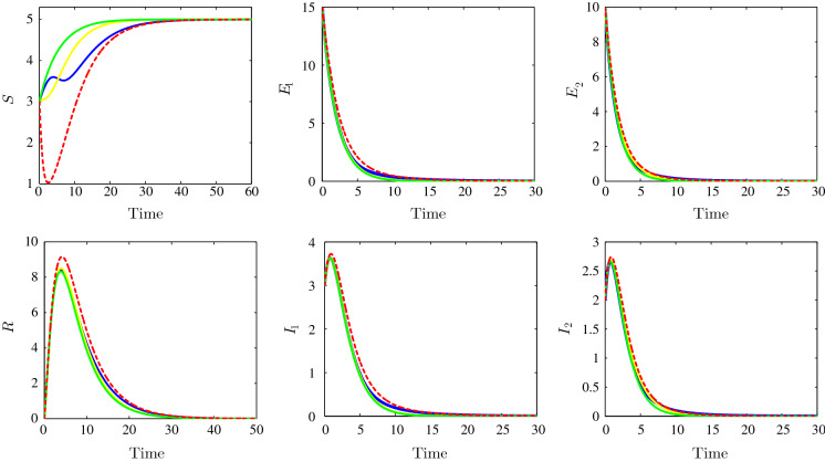
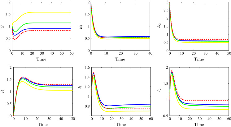
Figure 2 shows the behaviour of the infection for the following parameter values: $\Lambda =1$, $\alpha =0.17$, $\beta =0.15$, ${\gamma }_1=0.3$, ${\gamma }_2=0.4$, ${\mu }_1=0.65$, ${\mu }_2=0.75$, $\delta =0.2$, ${\omega }_1=0.4$, ${\omega }_2=0.6$, ${\omega }_3=4.5$, ${\omega }_4=5.8$, ${\chi }_1=2.5$, ${\chi }_2=3$, ${\chi }_3=6.5$, ${\chi }_4=5$, ${\alpha }_1=2.5$ and ${\alpha }_2=3$. We clearly see that the solutions of the system, under the various suggested incidence functions (bilinear, Beddington–DeAngelis, Crowley–Martin and non-monotonic functions), converge towards the same disease-free equilibrium point ${\mathcal{E}}_f=(5,0,0,0,0,0)$. In this situation, the nature of the incidence function has no effect on the steady-state value. Consequently, it was remarked that the disease-free equilibrium first nonzero component depends only on the birth and death rates of the susceptible individuals and does not depend, in any way, on the incidence functions parameters. Here, the disease dies out, the susceptible reaches their maximum value, and the other variables vanish. With the chosen parameters, we can easily calculate the two- strain basic reproduction numbers; in our case, we will have $R_0^1=0.6$ and $R_0^2=0.5263$ for the bilinear incidence functions case; we will have also $R_0^1=0.1$ and $R_0^2=0.6579$ for the Beddington–DeAngelis incidences case; $R_0^1=0.1154$ and $R_0^2=0.1645$ are calculated for Crowley–Martin incidence functions case, and finally, we have $R_0^1=0.6$ and $R_0^2=0.5263$ for the non-monotonic incidence functions case. In all these cases, we have the basic reproduction number $R_0$ is less than unity which is consistent with the theoretical result concerning the stability of the disease-free equilibrium ${\mathcal{E}}_f$.

Fig. 2.

Time evolution of susceptible (top left), the strain 1 latent individuals (top middle), the strain 2 latent individuals (top right), the recovered (bottom left), the strain 1 infectious individuals (bottom middle) and the strain 2 infectious individuals (bottom right) illustrating the stability of the disease-free equilibrium ${\mathcal{E}}_f$. The bilinear incidence functions (dotted red), Beddington–DeAngelis incidence functions (yellow), Crowley–Martin incidence functions (green) and the non-monotone incidence functions (blue). (Color figure online)

The stability of the endemic equilibria

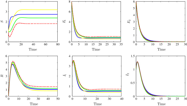
The dynamics behaviour concerning the stability of the strain 1 endemic equilibrium ${\mathcal{E}}_{s_1}$ is shown in Fig. 3. Indeed, we have chosen the following parameter values: $\Lambda =1$, $\alpha =0.5$, $\beta =0.12$, ${\gamma }_1=0.4$, ${\gamma }_2=0.3$, ${\mu }_1=0.4$, ${\mu }_2=0.75$, $\delta =0.2$, ${\omega }_1=0.4$, ${\omega }_2=0.85$, ${\omega }_3=1.5$, ${\omega }_4=0.05$, ${\chi }_1=4$, ${\chi }_2=3.5$, ${\chi }_3=0.3$, ${\chi }_4=0.05$, ${\alpha }_1=2$ and ${\alpha }_2=1.5$. For the bilinear incidence functions case, the solution converges towards the strain 1 endemic equilibrium (1.8, 1.0667, 0, 0.7111, 0, 1.4222) and with the chosen parameters we have $R_0^1=2.7778$ and $R_0^2=0.3789$. For the model with Beddington–DeAngelis, we observe the convergence towards $(3.1788,0.6071,0,0.4047,0,0.8094)$ and we have $R_0^1=11.1111$ and $R_0^2=0.3609$; for the third case, Crowley–Martin incidence type, we observe the convergence towards the equilibrium (2.3664, 0.8779, 0, 0.5852, 0, 1.1705) and we have $R_0^1=11.1111$ and $R_0^2=0.1024$. For the last non-monotonic incidence functions case, we see in the figure the convergence towards the steady state (2.7223, 0.7592, 0, 0.5062, 0, 1.0123) and we have $R_0^1=2.7778$ and $R_0^2=0.3789$. We remark that, for the all four cases, the strain 1 basic reproduction number $R_0^1$ is greater than unity while the other strain 2 basic reproduction number $R_0^2$ is less than one which confirms our theoretical findings concerning the stability of the strain 1 endemic equilibrium ${\mathcal{E}}_{s_1}$. This endemic equilibrium is characterized by the vanishing the strain 2 latent and infectious individuals.

Fig. 3.

Time evolution of susceptible (top left), the strain 1 latent individuals (top middle), the strain 2 latent individuals (top right), the recovered (bottom left), the strain 1 infectious individuals (bottom middle) and the strain 2 infectious individuals (bottom right) illustrating the stability of the strain 1 endemic equilibrium ${\mathcal{E}}_{s_1}$. The bilinear incidence functions (dotted red), Beddington–DeAngelis incidence functions (yellow), Crowley–Martin incidence functions (green) and the non-monotone incidence functions (blue). (Color figure online)

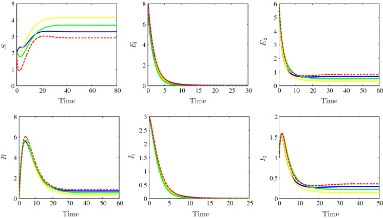
The strain 2 endemic equilibrium ${\mathcal{E}}_{s_2}$ stability is illustrated in Fig. 4. In this figure, the following parameters are chosen: $\Lambda =1$, $\alpha =0.2$, $\beta =0.4$, ${\gamma }_1=0.4$, ${\gamma }_2=0.3$, ${\mu }_1=1$, ${\mu }_2=0.5$, $\delta =0.2$, ${\omega }_1=0.4$, ${\omega }_2=0.85$, ${\omega }_3=1.5$, ${\omega }_4=0.05$, ${\chi }_1=4$, ${\chi }_2=3.5$, ${\chi }_3=0.3$, ${\chi }_4=0.05$, ${\alpha }_1=2$ and ${\alpha }_2=1.5$. We observe the convergence of the solution towards the steady state (2.9167, 0, 0.8333, 0, 0.3571, 0.8928) for the bilinear incidence functions case and with the adopted parameters we have $R_0^1=0.5556$ and $R_0^2=1.7143$. For the model with Beddington–DeAngelis, we observe the convergence towards $(4.1559,0,0.3376,0,0.1447,0.3617)$ and we have $R_0^1=0.5291$ and $R_0^2=6.8571$; for the third case, Crowley–Martin incidence type, we observe the convergence towards the equilibrium (3.6876, 0, 0.5250, 0, 0.2250, 0.5624) and we have $R_0^1=0.1502$ and $R_0^2=6.8571$. For the last non-monotonic incidence functions case, we see in the figure the convergence towards the steady state (3.2918, 0, 0.6833, 0, 0.2928, 0.7321) and we have $R_0^1=0.5556$ and $R_0^2=1.7143$. We remark that, for all the four cases, the strain 1 basic reproduction number $R_0^1$ is less than unity while the other strain 2 basic reproduction number $R_0^2$ is greater than one which is in good agreement with our theoretical findings concerning the stability of the strain 2 endemic equilibrium ${\mathcal{E}}_{s_2}$. From the components of this endemic equilibrium, we remark the clearance of the strain 1 latent and infectious individuals.

Fig. 4.

Time evolution of susceptible (top left), the strain 1 latent individuals (top middle), the strain 2 latent individuals (top right), the recovered (bottom left), the strain 1 infectious individuals (bottom middle) and the strain 2 infectious individuals (bottom right) illustrating the stability of the strain 2 endemic equilibrium ${\mathcal{E}}_{s_2}$. The bilinear incidence functions (dotted red), Beddington–DeAngelis incidence functions (yellow), Crowley–Martin incidence functions (green) and the non-monotone incidence functions (blue). (Color figure online)

The last endemic equilibrium ${\mathcal{E}}_t$ stability behaviour is depicted in Fig. 5 for $\Lambda =1$, $\alpha =0.6$, $\beta =0.6$, ${\gamma }_1=0.5$, ${\gamma }_2=0.5$, ${\mu }_1=0.15$, ${\mu }_2=0.15$, $\delta =0.2$, ${\omega }_1=1.2$, ${\omega }_2=0.06$, ${\omega }_3=1.2$, ${\omega }_4=0.06$, ${\chi }_1=0.4$, ${\chi }_2=0.05$, ${\chi }_3=0.4$, ${\chi }_4=0.05$, ${\alpha }_1=0.14$ and ${\alpha }_2=0.145$. As the previous figures, the dynamics for the different suggested incidence functions are illustrated. For the first one, the bilinear incidence function, we observe the convergence towards (0.8167, 0.5196, 0.6757, 0.7422, 0.9652, 1.2806) and with the adopted parameters we have $R_0^1=6.1224$ and $R_0^2=6.1224$. For Beddington–DeAngelis case, we observe the convergence towards $(1.5783,0.4888,0.4888,0.6983,0.6983,1.0474)$ and we have $R_0^1=23.5479$ and $R_0^2=23.5479$, for the third case, Crowley–Martin incidence type, we observe the convergence towards the equilibrium $(1.1353,0.5519,0.5523,0.7884,0.7890,1.1831)$ and we have $R_0^1=24.4898$ and $R_0^2=24.4898$. About the last non-monotonic incidence functions case, we see the convergence towards the steady state $(0.8982,0.5904,0.5815,0.8433,0.8309,1.2557)$ and we have $R_0^1=6.1224$ and $R_0^2=6.1224$. We remark that both the two-strain basic reproduction numbers $R_0^1$ and $R_0^2$ are greater than unity which confirms our theoretical findings concerning the stability of the last endemic equilibrium ${\mathcal{E}}_t$. This last endemic equilibrium is characterized by the persistence of all strains latent and infectious individuals. The numerical simulations confirm that the model with general incidence functions encompasses a large number of classical well-known incidence functions. Therefore, the generalized mathematical model can give a wide view about the stability of the different problem equilibria.

Fig. 5.

Time evolution of susceptible (top left), the strain 1 latent individuals (top middle), the strain 2 latent individuals (top right), the recovered (bottom left), the strain 1 infectious individuals (bottom middle) and the strain 2 infectious individuals (bottom right) illustrating the stability of the endemic equilibrium ${\mathcal{E}}_t$. The bilinear incidence functions (dotted red), Beddington–DeAngelis incidence functions (yellow), Crowley–Martin incidence functions (green) and the non-monotone incidence functions (blue). (Color figure online)

Comparison with COVID-19 clinical data

As we have mentioned in the introduction, the recent pandemic COVID-19 is a multi-strain infection. Therefore, the main interest of this subsection is to compare the numerical simulations resulting from our multi-strain epidemic model with COVID-19 clinical data. We have chosen to make our comparison the Moroccan clinical data during the year 2020 in the period between March 31 and June 20 [39, 40].

Figure 6 shows the time evolution of infected cases for the following parameter values: $\Lambda =1.5$, $\alpha =1.67$, $\beta =0.88$, $\delta =0.2$, ${\gamma }_1=1.05$, ${\gamma }_2=6.8$, ${\mu }_1=0.005$, ${\mu }_2=0.087$, ${\omega }_1=0.3$, ${\omega }_2=0.5$, ${\omega }_3=0.1$, ${\omega }_4=0.3$, ${\chi }_1=0.01$, ${\chi }_2=0.01$, ${\chi }_3=2.5$, ${\chi }_4=2.8$, ${\alpha }_1=0.0005$ and ${\alpha }_2=0.007$. We observe that a significant relationship exists between the curve representing the COVID-19 clinical data and the numerical simulations resulting from our mathematical model for the different incidence functions. Indeed, a good fit between the infected cases given by the mathematical model and the clinical data is observed. Each numerical result with the incidence function (bilinear, Beddington–DeAngelis, Crowley–Martin or non-monotonic function) fits well the clinical data, especially for a certain period of observation. Hence, the multi-strain mathematical model with generalized incidence functions is more appropriate to represent the studied disease.

Fig. 6.

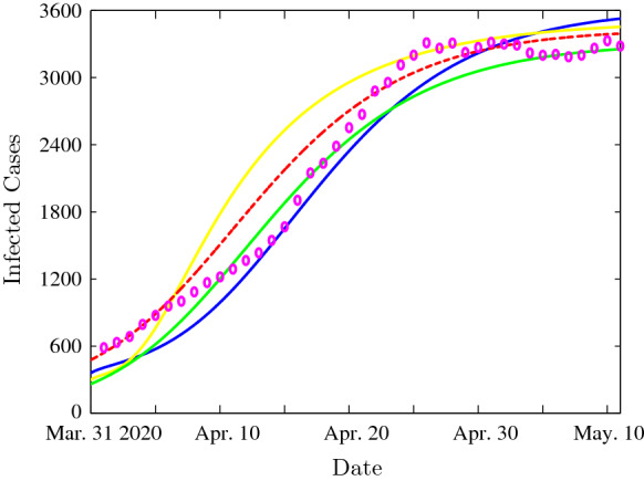
Time evolution of infected cases with the bilinear incidence functions (dotted red), Beddington–DeAngelis incidence functions (yellow), Crowley–Martin incidence functions (green) and the non-monotone incidence functions (blue). The clinical infected cases are illustrated by magenta circles. (Color figure online)

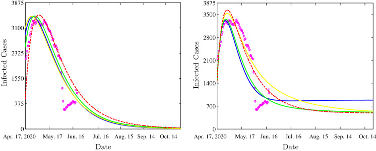
Figure 7 (left-hand side) shows the time evolution of infected cases for the following parameter values: $\Lambda =2$, $\alpha =0.01$, $\beta =0.01$, ${\gamma }_1=0.3$, ${\gamma }_2=0.4$, ${\mu }_1=0.07$, ${\mu }_2=0.5$, $\delta =0.2$, ${\omega }_1=0.5$, ${\omega }_2=0.6$, ${\omega }_3=0.1$, ${\omega }_4=0.3$, ${\chi }_1=1.5$, ${\chi }_2=2$, ${\chi }_3=0.7$, ${\chi }_4=3.7$, ${\alpha }_1=2$ and ${\alpha }_2=1.5$. We see that the solution of our model, under the various suggested incidence functions, converges towards the same disease-free equilibrium point ${\mathcal{E}}_f$. In this situation, the disease dies out, the susceptible reaches their maximum value and the other variables vanish. Within the chosen parameters, we can easily calculate the basic reproduction number; in our case we will have $R_0=0.23$ for the bilinear incidence functions case; we will have also $R_0=0.28$ for the Beddington–DeAngelis incidences case; $R_0=0.2$ are calculated for Crowley–Martin incidence functions case, and finally, we have $R_0=0.23$ for the non-monotonic incidence functions case.

Fig. 7.

Time evolution of infected cases with the bilinear incidence functions (dotted red), Beddington–DeAngelis incidence functions (yellow), Crowley–Martin incidence functions (green) and the non-monotone incidence functions (blue). The clinical infected cases are illustrated by magenta circles. (Color figure online)

The COVID-19 disease persistence case is illustrated in Fig. 7 (right-hand side). In this figure, the following parameters are chosen: $\Lambda =1.2$, $\alpha =0.1$, $\beta =0.52$, ${\gamma }_1=0.4$, ${\gamma }_2=0.1$, ${\mu }_1=0.23$, ${\mu }_2=0.2$, $\delta =0.03$, ${\omega }_1=0.5$, ${\omega }_2=0.6$, ${\omega }_3=0.1$, ${\omega }_4=0.3$, ${\chi }_1=1.5$, ${\chi }_2=4.5$, ${\chi }_3=0.7$, ${\chi }_4=0.12$, ${\alpha }_1=2$ and ${\alpha }_2=1.5$. We remark the convergence of the solution towards the endemic equilibrium for all the taken incidence functions. Indeed, for the case with bilinear incidence functions, we have the basic reproduction number is greater than unity $R_0=14.31$. For other cases, the basic reproduction number is also greater than one; indeed for Beddington–DeAngelis case, we have $R_0=36.6956$; for the third case, Crowley–Martin incidence type, we have $R_0=14.3113$. For the last non-monotonic incidence functions case, we have $R_0=14.3113$ which means that the disease persists. We can conclude that the numerical simulations fit well COVID-19 clinical data. Our numerical simulations reveal two scenarios of evolution for this pandemic, and within the first scenario the disease will die out. The other scenario happens when the basic reproduction number is greater than unity; in this case the disease will persist. In this situation, it will be important to eventually undertake some strategies like quarantine, isolation, wearing of masks, disinfection and if it will be possible vaccination.

The effect of quarantine strategy

In this subsection, we will study the effect of quarantine strategy in controlling the infection spread. To illustrate this effect and for simplicity, we will restrict ourselves to the case of the bilinear incidence function. More precisely, we will take the following incidence forms:

$$\begin{array}{c}\hfill f(S,I_1)=\alpha (1-u_1)S\text{and}g(S,I_2)=\beta (1-u_2)S,\\ \hfill \end{array}$$ 4.1

where $u_1$ stands for the efficiency of the quarantine strategy concerning the first strain infection rate, while $u_2$ represents the efficacy of the quarantine measures concerning the second-strain infection rate. Our numerical simulations will be performed in order to check the impact of the quarantine strategy for the case of the last endemic equilibrium.

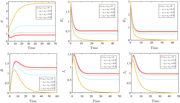
Figure 8 shows the time evolution of the susceptible, the two- strain latent individuals, two-strain infected individuals and the recovered for the following parameter values: $\Lambda =1$, $\alpha =0.6$, $\beta =0.6$, ${\gamma }_1=0.5$, ${\gamma }_2=0.5$, ${\mu }_1=0.15$, ${\mu }_2=0.15$, $\delta =0.2$ and for different values of the strategy controls $u_1$ and $u_2$. When no strategy is applied, we find the same result as in Fig. 5. By increasing the efficiency of the quarantine measures, we observe an interesting result. Indeed, the number of the susceptible individuals increases when $u_1$ and $u_2$ increase. For higher values of these two control parameters, the number of two-strain latent and infected individuals is reduced considerably, which means that the quarantine strategy can reduce the infection in efficient manner.

Fig. 8.

Effect of quarantine strategy on the SEIR model dynamics

Conclusion

In this paper, we have studied the global stability of two-strain epidemic model with two general incidence functions. The model included six compartments, namely the susceptible, two categories of the exposed, two categories of the infected and the removed individuals, this kind of model takes the abbreviation SEIR. We have established the existence, positivity and boundedness of solutions results which guarantee the wellposedness of our SEIR model. The disease-free equilibrium, the endemic equilibrium with respect to strain 1, the endemic equilibrium with respect to strain 2 and the endemic equilibrium with respect to both strains are given. By using an appropriate Lyapunov functionals, the global stability of the equilibria is established depending on the basic reproduction number $R_0$, the strain 1 reproduction number $R_0^1$ and the strain 2 reproduction number $R_0^2$. Numerical simulations are performed in order to confirm our different theoretical results. It was observed that the model with a generalized incidence function encompasses a large number of classical incidence functions and it can give more clear view about the equilibria stability. In addition, a numerical comparison between our model results and COVID-19 clinical data is conducted. We have observed a good fit between our numerical simulations and the clinical data which indicates that our multi-strain mathematical model can fit and predict the evolution of the infection. We have observed that strict quarantine measures can reduce significantly the infection spread. It is worthy to notice that a generalization form of this problem to a more complex compartmental model is proposed in Appendix of this paper. For this complex model, we have given its basic reproduction number and each strain reproduction number. Furthermore, the forms of the Lyapunov functionals for this complex compartmental model are also formulated.

Appendix

Multi-strain compartmental epidemiological model

The generalization of the problem to a more complex compartmental model with general incidence rates is formulated as follows

$$\begin{array}{c}\hfill (P)\left\{\begin{array}{cc}\hfill \frac{\mathrm{d}S}{\mathrm{d}t}& =\Lambda -\sum _{i=1}^{i=n}{f}_i(S,I_i)I_i-\delta S,\hfill \\ \hfill \frac{\mathrm{d}{E}_i}{\mathrm{d}t}& =f_i(S,I_i)I_i-({\gamma }_i+\delta )E_i,i=1,2,\dots ,n\hfill \\ \hfill \frac{\mathrm{d}{I}_i}{\mathrm{d}t}& ={\gamma }_i{E}_i-({\mu }_i+\delta )I_i,i=1,2,\dots ,n\hfill \\ \hfill \frac{\mathrm{d}R}{\mathrm{d}t}& =\sum _{i=1}^{i=n}{\mu }_i{I}_i-\delta R,\hfill \end{array}\right)\end{array}$$ A.1

with

$$\begin{array}{cc}& S(0)\ge 0,E_i(0)\ge 0,I_i(0)\ge 0,R(0)\ge 0,\hfill \\ \hfill & \forall i\in \{1,2,\dots ,n\}.\hfill \end{array}$$

This model contains $2n+2$ variables ($n\in {\mathbb{N}}^{\ast }$) that are: the susceptible individuals S, removed individuals R, n categories of latent individuals $E_1,E_2\dots ,E_n$ and n categories of infectious individuals $I_1,I_2,\dots ,I_n$. The parameter ${\displaystyle \frac{1}{\delta }}$ represents the average life expectancy of the population, ${\displaystyle \frac{1}{{\mu }_i}}$ represents the average infection period of strain i, ${\displaystyle \frac{1}{{\gamma }_i}}$ represents the average latency period of strain i. Finally, $f_i(S,I_i)$ represents the general incidence rate for the strain i and verifies the follows conditions:

$$\begin{array}{cc}& f_i(0,I_i)=0,\forall I_i\ge 0,i=1,2,\dots ,n\hfill \\ \hfill & \frac{\partial f_i(S,I_i)}{\partial S}>0,\forall S>0,\forall I_i\ge 0,i=1,2,\dots ,n\hfill \\ \hfill & \frac{\partial f_i(S,I_i)}{\partial I_i}\le 0,\forall S\ge 0,\forall I_i\ge 0,i=1,2,\dots ,n.\hfill \end{array}$$

Main steps of the global analysis

The model is well defined, all solutions with non-negative initial conditions exist, remain non-negative and bounded. Let N(t) be the total population, we have

$$\begin{array}{c}\hfill N(t)=S(t)+\sum _{i=1}^{i=n}{E}_i(t)+\sum _{i=1}^{i=n}{I}_i(t)+R(t).\end{array}$$ A.2

By adding all equations of the problem (P), we will have

$$\begin{array}{c}\hfill {\displaystyle \frac{\mathrm{d}N(t)}{\mathrm{d}t}=\Lambda -\delta N(t),}\end{array}$$ A.3

then,

$$\begin{array}{c}\hfill {\displaystyle N(t)=\frac{\Lambda }{\delta }+(N(0)-\frac{\Lambda }{\delta }){\mathrm{e}}^{-\delta t},}\end{array}$$ A.4

and consequently,

$$\begin{array}{c}\hfill {\displaystyle \underset{t\to +\infty }{lim}N(t)=\frac{\Lambda }{\delta }.}\end{array}$$ A.5

This means that the biological feasible region is given by

$$\begin{array}{cc}& \mathcal{H}=\{(S,E_1,E_2,\dots ,E_n,I_1,I_2,\dots ,I_n,R)\in {\mathbb{R}}_{+}^{2n+2}\text{such that}\hfill \\ \hfill & {\displaystyle S+\sum _{i=1}^{i=n}{E}_i+\sum _{i=1}^{i=n}{I}_i+R\le \frac{\Lambda }{\delta }\}}\hfill \end{array}$$ A.6

is positively invariant.

The basic reproduction number is given by

$$\begin{array}{c}\hfill R_0=\underset{i\in \{1,2,\dots ,n\}}{max}\left\{{\displaystyle \frac{f_i(\frac{\Lambda }{\delta },0){\gamma }_i}{({\gamma }_i+\delta )({\mu }_i+\delta )}}\right\}.\end{array}$$ A.7

and the strain i reproduction number is given by

$$\begin{array}{c}\hfill {\displaystyle R_0^i=\frac{f_i(\frac{\Lambda }{\delta },0){\gamma }_i}{({\gamma }_i+\delta )({\mu }_i+\delta )},i=1,2,\dots ,n.}\end{array}$$ A.8

By simple reasoning, we can easily prove that this problem has $2^n$ steady states.

It is clear that the disease-free equilibrium point ${\mathcal{E}}_f(\frac{\Lambda }{\delta },0,\dots ,0)$ is globally asymptotically stable if $R_0\le 1$.

In order to study the global stability for each equilibrium point ${\mathcal{E}}_{s_i}$ $(\forall i\in \{1,2,\dots ,n\})$, it appears that the Lyapunov functional can take the following form

$$\begin{array}{cc}& {\mathcal{L}}_i(S,E_1,E_2,\dots ,E_n,I_1,I_2,\dots ,I_n)\hfill \\ \hfill & {\displaystyle =S-S_{s_i}^{\ast }-{\int }_{S_{s_i}^{\ast }}^S\frac{f(S_{s_i}^{\ast },I_{i,s_i}^{\ast })}{f(X,I_{i,s_i}^{\ast })}\mathrm{d}X}\hfill \\ \hfill & +\sum _{i=1}^{i=n}{E}_{i,s_i}^{\ast }\left({\displaystyle \frac{E_i}{E_{i,s_i}^{\ast }}-ln\left({\displaystyle \frac{E_i}{E_{i,s_i}^{\ast }}}\right)-1}\right)\hfill \\ \hfill & +\sum _{i=1}^{i=n}\frac{{\gamma }_i+\delta }{{\gamma }_i}{I}_{i,s_i}^{\ast }\left(\frac{I_i}{I_{i,s_i}^{\ast }},-,ln,\left(\frac{I_i}{I_{i,s_i}^{\ast }}\right),-,1\right).\hfill \end{array}$$ A.9

The functions $f_i$ are assumed to verify the following condition:

$$\begin{array}{c}\hfill \left(1,-,\Gamma \right)\left({\displaystyle \frac{1}{\Gamma }-\frac{I_i}{I_{i,s_i}^{\ast }}}\right)\le 0,\forall S,I_i>0i=1,2,\dots ,n,\end{array}$$

with ${\displaystyle \Gamma =\prod _{i=1}^{i=n}\frac{f_i(S,I_{i,s_i}^{\ast })}{f_i(S_{s_i}^{\ast },I_{i,s_i}^{\ast })}\frac{f_j(S_{s_i}^{\ast },I_{j,s_j}^{\ast })}{f_j(S,I_{j,s_j}^{\ast })}}$ such that $I_{i,s_i}^{\ast }\ne 0$, $I_{j,s_j}^{\ast }\ne 0,i\in \{1,2,\dots ,n\},j\in \{1,2,\dots ,n\}\text{and}i\ne j$.

Compliance with ethical standards

Conflict of interest

The authors declare that they have no conflict of interest.

References

- 1.Kermack WO, McKendrick AG. A contribution to the mathematical theory of epidemics. Proc. R. Soc. Lond. A. 1927;115:700–721. doi: 10.1098/rspa.1927.0118. [DOI] [Google Scholar]
- 2.Munster VJ, de Wit E, van den Brand JMA, Herfst S, Schrauwen EJA, Bestebroer TM, van de Vijver D, Boucher CA, Koopmans M, Rimmelzwaan GF, et al. Pathogenesis and transmission of swine-origin a (H1N1) influenza virus, ferrets. Science. 2009;325:481–483. doi: 10.1126/science.1177127. [DOI] [PMC free article] [PubMed] [Google Scholar]
- 3.Layne SP, Monto SP, Taubenberger JK. Pandemic influenza: an inconvenient mutation. Science (NY) 2020;323:1560–1561. doi: 10.1126/science.323.5921.1560. [DOI] [PMC free article] [PubMed] [Google Scholar]
- 4.Gobalenya AE, Baker SC, Baric RS, de Groot RJ, Drosten C, Gulyaeva AA, et al. The species severe acute respiratory syndrome-related coronavirus: classifying 2019-nCoV and naming it SARS-CoV-2. Nat. Microbiol. 2020;5:536–544. doi: 10.1038/s41564-020-0695-z. [DOI] [PMC free article] [PubMed] [Google Scholar]
- 5.Golub JE, Bur S, Cronin W, Gange S, Baruch N, Comstock G, Chaisson RE. Delayed tuberculosis diagnosis and tuberculosis transmission. Int. J. Tuber. 2006;10:24–30. [PubMed] [Google Scholar]
- 6.Brenchley JM, Price DA, Schacker TW, Asher TE, Silvestri G, Rao S, et al. Microbial translocation is a cause of systemic immune activation in chronic HIV infection. Nat. Med. 2006;12:1365–1371. doi: 10.1038/nm1511. [DOI] [PubMed] [Google Scholar]
- 7.Gubler DJ. Dengue and dengue hemorrhagic fever. Clin. Microbiol. Rev. 1998;11:480–96. doi: 10.1128/CMR.11.3.480. [DOI] [PMC free article] [PubMed] [Google Scholar]
- 8.Li MY, Muldowney JS. Global stability for the SEIR model in epidemiology. Math. Biosci. 1995;125:155–164. doi: 10.1016/0025-5564(95)92756-5. [DOI] [PubMed] [Google Scholar]
- 9.Li, M.Y., Wang, L.L.: Global stability in some SEIR epidemic models. In: Castillo-Chavez, C., Blower, S., van den Driessche, P., Kirschner, D., Yakubu, A.A. (eds.) Mathematical Approaches for Emerging and Reemerging Infectious Diseases: Models, Methods, and Theory. The IMA Volumes in Mathematics and its Applications, vol 126. Springer, New York, NY (2002)
- 10.Huang G, Takeuchi Y, Ma W, Wei D. Global stability for delay SIR and SEIR epidemic models with nonlinear incidence rate. Bull. Math. Biol. 2010;72:1192–1207. doi: 10.1007/s11538-009-9487-6. [DOI] [PubMed] [Google Scholar]
- 11.Bentaleb D, Amine S. Lyapunov function and global stability for a two-strain SEIR model with bilinear and non-monotone. Int. J. Biomath. 2019;12:1950021. doi: 10.1142/S1793524519500219. [DOI] [Google Scholar]
- 12.Meskaf A, Khyar O, Danane J, Allali K. Global stability analysis of a two-strain epidemic model with non-monotone incidence rates. Chaos Sol. Frac. 2020;133:109647. doi: 10.1016/j.chaos.2020.109647. [DOI] [Google Scholar]
- 13.Hattaf K, Yousfi N, Tridane A. Mathematical analysis of a virus dynamics model with general incidence rate and cure rate. Nonlinear anal. Real World Appl. 2012;13:1866–1872. doi: 10.1016/j.nonrwa.2011.12.015. [DOI] [Google Scholar]
- 14.Hattaf K, Khabouze M, Yousfi N. Dynamics of a generalized viral infection model with adaptive immune response. Int. J. Dyn. Control. 2015;3:253–261. doi: 10.1007/s40435-014-0130-5. [DOI] [Google Scholar]
- 15.Ji C, Jiang D. Threshold behaviour of a stochastic SIR model. Appl. Math. Model. 2014;38:5067–5079. doi: 10.1016/j.apm.2014.03.037. [DOI] [Google Scholar]
- 16.Wang JJ, Zhang JZ, Jin Z. Analysis of an SIR model with bilinear incidence rate. Nonlinear Anal. Real World Appl. 2010;11:2390–2402. doi: 10.1016/j.nonrwa.2009.07.012. [DOI] [Google Scholar]
- 17.Liu X, Yang L. Stability analysis of an SEIQV epidemic model with saturated incidence rate. Nonlinear Anal. Real World Appl. 2012;13:2671–2679. doi: 10.1016/j.nonrwa.2012.03.010. [DOI] [Google Scholar]
- 18.Zhao Y, Jiang D. The threshold of a stochastic SIRS epidemic model with saturated incidence. Appl. Math. Lett. 2014;34:90–93. doi: 10.1016/j.aml.2013.11.002. [DOI] [Google Scholar]
- 19.Beddington JR. Mutual interference between parasites or predators and its effect on searching efficiency. J. Anim. Ecol. 1975;44:331–341. doi: 10.2307/3866. [DOI] [Google Scholar]
- 20.Cantrell RS, Cosner C. On the dynamics of predator-prey models with the Beddington–DeAngelis functional response. J. Math. Anal. Appl. 2001;257:206–222. doi: 10.1006/jmaa.2000.7343. [DOI] [Google Scholar]
- 21.DeAngelis DL, Goldstein RA, O’Neill RV. A model for tropic interaction. Ecology. 1975;56:881–892. doi: 10.2307/1936298. [DOI] [Google Scholar]
- 22.Crowley PH, Martin EK. Functional responses and interference within and between year classes of a dragonfly population. J. North. Am. Benth. Soc. 1989;8:211–221. doi: 10.2307/1467324. [DOI] [Google Scholar]
- 23.Liu XQ, Zhong SM, Tian BD, Zheng FX. Asymptotic properties of a stochastic predator-prey model with Crowley–Martin functional response. J. Appl. Math. Comput. 2013;43:479–490. doi: 10.1007/s12190-013-0674-0. [DOI] [Google Scholar]
- 24.Zhou X, Cui J. Global stability of the viral dynamics with Crowley–Martin functional response. Bull. Korean Math. Soc. 2011;48:555–574. doi: 10.4134/BKMS.2011.48.3.555. [DOI] [Google Scholar]
- 25.Hattaf K, Mahrouf M, Adnani J, Yousfi N. Qualitative analysis of a stochastic epidemic model with specific functional response and temporary immunity. Phys. A. 2018;490:591–600. doi: 10.1016/j.physa.2017.08.043. [DOI] [Google Scholar]
- 26.Hattaf K, Yousfi N. Global dynamics of a delay reaction–diffusion model for viral infection with specific functional response. Comput. Appl. Math. 2015;34:807–818. doi: 10.1007/s40314-014-0143-x. [DOI] [Google Scholar]
- 27.Hattaf K, Yousfi N, Tridane A. Stability analysis of a virus dynamics model with general incidence rate and two delays. Appl. Math. Comput. 2013;221:514–521. [Google Scholar]
- 28.Lotfi EM, Maziane M, Hattaf K, Yousfi N. Partial differential equations of an epidemic model with spatial diffusion. Int. J. Part. Differ. Equ. 2014;2014:6. [Google Scholar]
- 29.Maziane M, Lotfi EM, Hattaf K, Yousfi N. Dynamics of a class of HIV infection models with cure of infected cells in eclipse stage. Acta. Bioth. 2015;63:363–380. doi: 10.1007/s10441-015-9263-y. [DOI] [PubMed] [Google Scholar]
- 30.Capasso V, Serio G. A generalization of the Kermack–McKendrick deterministic epidemic model. Math. Biosci. 1978;42:43–61. doi: 10.1016/0025-5564(78)90006-8. [DOI] [Google Scholar]
- 31.Liu WM, Levin SA, Iwasa Y. Influence of nonlinear incidence rates upon the behavior of sirs epidemiological models. J. Math. Biol. 1986;23:187–204. doi: 10.1007/BF00276956. [DOI] [PubMed] [Google Scholar]
- 32.Hethcote HW, Van den Driessche P. Some epidemiological models with nonlinear incidence. J. Math. Biol. 1991;29:271–287. doi: 10.1007/BF00160539. [DOI] [PubMed] [Google Scholar]
- 33.Derrick WR, Van den Driessche P. A disease transmission model in a nonconstant population. J. Math. Biol. 1993;31:495–512. doi: 10.1007/BF00173889. [DOI] [PubMed] [Google Scholar]
- 34.Ruan S, Wang W. Dynamical behavior of an epidemic model with a nonlinear incidence rate. J. Diff. Equ. 2003;188:135–163. doi: 10.1016/S0022-0396(02)00089-X. [DOI] [Google Scholar]
- 35.He S, Peng Y, Sun K. SEIR modeling of the COVID-19 and its dynamics. Nonlinear Dyn. 2020 doi: 10.1007/s11071-020-05743-y. [DOI] [PMC free article] [PubMed] [Google Scholar]
- 36.Rohith G, Devika KB. Dynamics and control of COVID-19 pandemic with nonlinear incidence rates. Nonlinear Dyn. 2020 doi: 10.1007/s11071-020-05774-5. [DOI] [PMC free article] [PubMed] [Google Scholar]
- 37.Minoza, J.M.A., Sevilleja, J.E.A., de Castro, R., Caoili, S.E., Bongolan, V.P.: Protection after quarantine: insights from a Q-SEIR model with nonlinear incidence rates applied to COVID-19. medRxiv (2020). 10.1101/2020.06.06.20124388
- 38.Hale JK, Lunel SMV, Verduyn LS, Lunel SMV. Introduction to Functional Differential Equations. New York: Springer; 1993. [Google Scholar]
- 39.World Health Organization, Coronavirus World Health Organization 19, (2020). https://www.who.int/health-topics/coronavirus
- 40.Statistics of Moroccan Health Ministry on COVID-19. https://www.sante.gov.ma/