

Abstract
Gravity waves in Mars’s atmosphere strongly affect the general circulation as well as middle atmospheric cloud formation, but the climatology and sources of gravity waves in the lower atmosphere remain poorly understood. At Earth, the statistical variance in satellite observations of thermal emission above the instrumental noise floor has been used to enable measurement of gravity wave activity at a global scale. Here is presented an analysis of variance in calibrated radiance at 15.4 μm (635-665 cm−1) from off-nadir and nadir observations by the Mars Climate Sounder (MCS) on board Mars Reconnaissance Orbiter (MRO); a major expansion in the observational data available for validating models of Martian gravity wave activity. These observations are sensitive to gravity waves at 20-30 km altitude with wavelength properties (λh=10-100 km, λz > 5 km) that make them likely to affect the dynamics of the middle and upper atmosphere. We find that: (1) strong, moderately intermittent gravity wave activity is scattered over the tropical volcanoes and throughout the middle to high latitudes of both hemispheres during fall and winter, (2) gravity wave activity noticeably departs from climatology during regional and global dust storms; and (3) strong, intermittent variance is observed at night in parts of the southern tropics during its fall/winter, but frequent CO2 ice clouds prevents unambiguous attribution to GW activity. The spatial distribution of wave activity is consistent with topographic sources being dominant, but contributions from boundary layer convection and other convective processes are possible.
Keywords: Mars, atmosphere, Atmospheres, dynamics, Infrared observations, Meteorology, Mars, climate
1. Introduction
Gravity waves (GW) enable the circulation near Earth’s surface to affect the middle and upper atmospheric circulation by transporting heat and momentum through strongly stratified atmospheric layers (Holton et al., 1995; Yamanaka, 1995; Fritts and Alexander, 2003; Yiğit and Medvedev, 2015). Along with planetary waves, GW help maintain a seasonally reversing circulation in the mesosphere, excite the quasi-biennial oscillation, and control the stability of the polar stratospheric vortices (e.g., Holton, 1982; Dunkerton, 1997; Albers and Birner, 2014). GW also stimulate the formation of polar stratospheric clouds (e.g., Fritts et al., 1993; Chandran et al., 2009; Hoffmann et al., 2017).
GW also are important for the atmospheric dynamics of Mars, where GW drag is thought to close the westerly winter jets and drive a downwelling circulation that heats the winter polar middle atmosphere significantly above radiative equilibrium (e.g., Jaquin, 1989; Barnes, 1990; Medvedev et al., 2011b,a; Kuroda et al., 2015, 2016). GW drag, along with analogous planetary wave and tidal drag, may be especially potent during global dust storm activity (Kuroda et al., 2009). The observation of middle atmospheric polar warming (at the winter solstitial and equinoctial poles) (Conrath et al., 2000; McCleese et al., 2008; McCleese et al., 2010) and its higher magnitude during dust storms (Wilson, 1997; Smith, 2004) has raised further interest in Martian GW and in alternative mechanisms for generating polar warming, such as radiative forcing by tropical water ice clouds (Wilson et al., 2008). Local temperature fluctuations created by GW also may enable CO2 ice clouds to form high in Mars’s middle atmosphere, where mean temperatures are too warm for CO2 to condense (Spiga et al., 2012; Yiğit et al., 2015, 2018). GW also generate significant density fluctuations in the upper atmosphere experienced by spacecraft aerobraking or making in situ observations of Mars’s upper atmosphere (Tolson et al., 2005; Creasey et al., 2006b; Fritts et al., 2006). These fluctuations drive significant seasonal and diurnal variability in Mars’s turbopause (Yamanaka, 1995; Imamura et al., 2016; Slipski et al., 2018) and strong heating/cooling of the thermosphere by mechanical dissipation of the waves (Parish et al., 2009; Medvedev and Yiğit, 2012; Walterscheid et al., 2013). GW thus have broad implications for dynamics, chemistry, atmospheric evolution, and the successful execution of aerobraking/aerocapture maneuvers by future missions to Mars (e.g., Tolson et al., 2005).
The dynamical effects of GW depend on their characteristics. High-frequency GW (those with frequencies less than but within a factor of 10 of the Brunt-Väisälä frequency, N) are most energy-efficient at transporting momentum and have short horizontal wavelengths (typically << 100 km) and long vertical wavelengths (typically >> 10 km) (Gong et al., 2012). The horizontal scale of these waves is below the resolution typically resolved by global climate models (GCM) (Kuroda et al., 2015, 2016). As long as they are long enough to avoid internal reflection and have non-zero phase speeds, high-frequency GW are most likely to propagate to the middle and/or upper atmospheres and affect the circulation there (Kuroda et al., 2015; Imamura et al., 2016). Low-frequency GW carry less momentum and tend to be attenuated lower in the atmosphere.
GW wavelength, frequency, and phase speed characteristics are broadly determined by their sources. GW from topographic sources can have a variety of frequencies but have near-zero phase speeds. GW also can be generated by jet/front instabilities/geostrophic adjustment (low-frequency with diverse phase speeds) or convection (low-high frequency with diverse phase speeds) (Fritts and Alexander, 2003). Thus, even high-frequency convectively-generated GW may propagate differently than topographically-generated GW, though it remains controversial which source more strongly impacts middle and upper atmospheric dynamics in Earth’s atmosphere.
Over the last two decades, satellite remote sensing has improved characterization of the global variability, climatology, and spectral diversity of GW in the Earth’s atmosphere. This improvement has come from using small-scale fluctuations in radiance at temperature-sensitive frequencies above the instrumental noise floor and/or fluctuations in retrieved vertical profiles of temperature/density etc. as measures of GW activity (e.g., Wu and Waters, 1996). The sensitivity of satellite observations to particular parts of the GW spectrum depends on the observational geometry and the transparency of the atmosphere at the wavelength being observed (Wu et al., 2006). Limb sounding instruments are sensitive to long horizontal wavelength, short vertical wavelength GW, which are low frequency. Nadir and off-nadir observations tend to be sensitive to higher frequency GW. (See Section 2.1 for discussion of the basic principles and terminology.)
Lower and middle atmospheric GW activity at Mars has been principally studied at the limb, either by radio occultation or thermal infrared limb sounding (Creasey et al., 2006a; Heavens et al., 2010; Wright, 2012; Ando et al., 2012; Tellmann et al., 2013). While the sensitivity of these techniques to vertical wavelength varies, their horizontal weighting functions can be > 200 km, which limits sensitivity to shorter wavelength GW and enhances sensitivity to Mars’s high amplitude thermal tides. One exception is Imamura et al. (2007), which analyzed the atmospheric energy spectrum of Mars inferred from nadir observations of the 15 μm CO2 band by the Thermal Emission Spectrometer (TES) on board Mars Global Surveyor (MGS) and found that the energy spectrum decayed at higher wavenumber (shorter wavelength) less than expected. Imamura et al. (2007) therefore inferred significant GW activity at those wavelengths and/or mesoscale thermal structures related to dust storm activity and clouds. Another exception is Altieri et al. (2012), which detected GW activity in the southern mid-high latitudes around northern fall equinox from mesoscale variance in O2 near-infrared dayglow from on-planet observations by Observatoire pour la Minéralogie, l’Eau, les Glaces et l’Activité (OMEGA) on board Mars Express.
In this study, we investigate the global variability of GW activity in the lower atmosphere based on off-nadir and nadir observations (collectively on-planet observations) by the Mars Climate Sounder (MCS) on board Mars Reconnaissance Orbiter (MRO) (McCleese et al., 2007). MCS on-planet observations have three important advantages for GW studies at Mars. First, they are primarily sensitive to high-frequency GW, as will be demonstrated in the next section. Second, they now span a longer record than is available for the Thermal Emission Spectrometer (TES) on board Mars Global Surveyor (Smith, 2004, 2009). Third, the switch from nadir to off-nadir observations necessitated by actuator difficulties early in MRO-MCS operations (McCleese et al., 2010) allows the spatial and temporal variability of different parts of the high-frequency GW spectrum to be compared and contrasted over a portion of the seasonal cycle. We also consider the circumstances under which small-scale temperature variance may not be a good GW activity proxy.
The outline of this paper is as follows. In section 2, we outline the methodological background of our approach to measuring GW activity and its specific application in this study. In section 3, we analyze the GW activity dataset described in the previous section. In section 4, we compare the results with past observations and modeling and attempt to infer likely GW sources from the results of the study. In section 5, the results of the study are summarized. Appendices A-C describe analyses relating to biases of our approach or comparison with modeling that otherwise would divert the flow of the main body of the paper.
2. Methods
2.1. General Method
Wu and Waters (1996) demonstrated that the horizontal resolution of satellite instruments at the Earth was now good enough to enable temperature fluctuations associated with upward propagating GW to be sampled by looking at the variations in temperature between closely spaced observations.
Consider a GW restricted to a plane defined by a dimension x parallel to the surface and a dimension z perpendicular to it and observed at a time t. The temperature perturbation, , associated with it takes the form:
| (1) |
where is a normalized amplitude, k and m are the horizontal and vertical wavenumbers, and w is the ground-relative frequency (Fritts and Alexander, 2003).
If a single wave is observed over a period of time much shorter than the inverse of its frequency (≈ 100 s for a wave with a frequency of N), the resulting temperature perturbation field is a series of tilted perturbations that increase in amplitude with height. The angle of tilt can be related either to its intrinsic frequency (its frequency relative to the ambient wind field) or the relative magnitude of its horizontal and vertical wavenumbers. In this way, GW perturb the background temperature field set by radiative-convective balance and larger-scale waves/tides. When scattering is neglected, an observation of emitted radiance (Iλ) from a planetary atmosphere/surface at a given wavelength, λ, can be defined by its vertical weighting function:
| (2) |
which follows from:
| (3) |
where Bλ(T) is the Planck function at temperature T, Tλ(l) is the atmospheric transmittance along a path l between the surface at l = 0 and the point of observation at ∞, and Tλ(0)l,∞ is the transmittance at the surface (e.g. Liou, 2002). When the atmospheric path viewed is optically thick, the term outside the integral, known as the surface contribution, vanishes, so that the radiance is simply a convolution of the Planck function with the weighting function. In limb geometry, the surface contribution likewise vanishes and Eq. 3 is typically re-written for a geometry centered on the point at which the optical path is closest to the planetary surface. This point is called the tangent point or tangent height, when referring to the poin’s altitude relative to the surface (e.g., Nakajima et al., 2002). For nadir geometry, l reduces to the height coordinate z.
Eq. 3 also can be written in terms of brightness temperature, Tb,λ, and so that the observed brightness temperature is dependent on temperature along a horizontal dimension parallel to the surface x. In the optically thick limit, we have:
| (4) |
The contribution of GW perturbations to brightness temperature will change as each observation samples the horizontal and vertical variability of a given wave along a different atmospheric path. Indeed, the sensitivity of the observed brightness temperature to the wave will depend on how well the breadth of the vertical weighting function and the horizontal baseline of the observation matches the wavelength of the wave. To illustrate this, Fig. 1 shows an example observation for a notional instrument in which the vertical wavelength is twice the full-width half-maximum (FWHM) of the vertical weighting function. Because typical lower atmosphere GW perturbations observed at the Earth or Mars are on the order of 1 K, an amplitude of 1 K was chosen for the example GW (Fritts et al., 1988; Creasey et al., 2006a).
Figure 1:

Schematic showing the sensitivity of notional satellite observations to a GW with a horizontal wavelength of 100 km, a vertical wavelength of 32.8 km, and an amplitude at the surface of 1 K: (a) Temperature field in the x-z plane (color contours) with thin black traces showing the weighting functions for the observation (plotted in relative units) staggered every 10 km along the x-axis and thick black trace indicating the 150 K isotherm to illustrate the wave pattern; (b) Brightness temperature (K) calculated from the temperature field convolved with the vertical wavefunctions and averaged horizontally at 10 km resolution.
Wu and Waters (1996) therefore argued that GW perturbations could be measured along a horizontal baseline with some number of observations, M, by calculating the variance of linearly detrended brightness temperatures, where a and b are the slope and intercept of the linear fit:
| (5) |
Wu and Waters (1996) analyzed microwave limb observations from scanning in tangent height in the course of spacecraft motion. Therefore, the observations were detrended based on tangent height, but this was equivalent to a horizontal detrending as it presumably ”removed…the tangent pressure dependence and large-scale wave modulations” (Wu and Waters, 1996).
The uncertainty in is proportional to:
| (6) |
where σTerr is the uncertainty in an individual measured brightness temperature.
For notational convenience, we will refer to as ΩGW, as ∊GW, normalized by the square of the mean temperature as .and Following Wu and Waters (1996), the uncertainty in the mean ΩGW is proportional to the quotient of ∊GW and square root of the number of observations in the spatial averaging bin.
The normalization by the square of the mean temperature creates a quantity proportional to the specific energy of the gravity waves. For example, the wave potential energy per unit mass, Ep can be approximated as:
| (7) |
where g is the acceleration due to gravity (Ern et al., 2004; Creasey et al., 2006a).
And the vertical flux of horizontal momentum flux can be approximated as:
| (8) |
where λz and λh are the vertical and horizontal wavelengths and ρ is the air density (Ern et al., 2004).
These expressions are approximate, because they adopt the mid-frequency approximation that the frequency of the wave is intermediate between N and the Coriolis parameter f, and do not account for the fact that metrics like ΩGW do not conserve the true amplitude of the wave but have variable sensitivity based on their weighting functions and GW characteristics. However, they are helpful for understanding the relationship of the metrics derived from satellite observations to atmospheric dynamics and comparing observations to models.
Note that is a useful parameter to keep in mind, because for λz sufficiently smaller than 120 km in Mars’s atmosphere, the intrinsic frequency, ŵ (wind-relative frequency of a GW), is:
| (9) |
2.2. The MCS Calibrated Radiance Dataset
MCS has observed Mars since September 2006 (Ls=111° of Mars Year (MY) 28 in the sense of Clancy et al. (2000); Piqueux et al. (2015)). MCS observes radiance in nine channels in the visible/near-infrared and thermal infrared (33,000-220 cm−1) from scans of Mars and its atmosphere that include both the forward and aft limb as well as along and to both sides of the track of the MRO spacecraft (McCleese et al., 2007). Each spectral channel consists of a linear array of 21 thermopile detectors, each with a field of view (FOV) of 3.6 × 6.1 mrad. When observing forward and in-track, the FOV corresponds to an along-track resolution of ≈ 1 km in the nadir and ≈ 2.9 km at the center of the detector array at the nominal off-nadir observational angle of 8.9° below the limb, which is smeared to ≈ 6 km by spacecraft motion during the 2.048 s integration time of individual observations (Hayne et al., 2012; Bandfield et al., 2013; Hayne et al., 2014). The width of an individual detector is ≈ 1.5 km. When observing in-track with MRO, MCS radiance observations are aligned just west of north on the dayside and just west of south on the nightside, except at the poles, which makes them primarily sensitive to variability in the north-south direction.
The nominal observational strategy was to observe the nadir (with two measurements that overlapped in the direction of the orbital track), the forward limb in-track (eight measurements), to space, and then to the nadir again at local times near 3:00 LST (nightside) and 15:00 LST (dayside). Occasionally, off-nadir observations were also included. The nadir and limb observations were then calibrated against observations of space and of an instrumental blackbody, as described by Henderson and Sayfi (2007).
On 10 December 2006 (Ls=168° of MY 28), the instrument’s elevation actuator began to be unable to accurately scan to nadir; all nadir observations were suspended by 9 February 2007 (Ls=180° of MY 28). The substitution of off-nadir observations (with a nominal angle of 8.9° below the limb/surface incidence angle of 67° off-nadir) into the observation cycle began after Ls=329° of MY 28 (11 October 2007). Since then, regular campaigns of cross-track observations, coordinated observations with other spacecraft, mechanical tests, and MRO spacecraft maneuvers can reduce the number of off-nadir observations.
2.3. Sensitivity of A3 On-Planet Views to Elevation, Wave Characteristics, and Aerosol
This study focuses on the on-planet views made by MCS in the A3 channel (635-665 cm−1). Observing near the center of the 15 μm CO2 band, this channel is analogous to the T15 channel of the Viking Orbiter’s Infrared Thermal Mapper (IRTM), whose broad weighting function peaks around 25 km above the surface (Wilson and Richardson, 2000). Under most circumstances, the atmosphere in this spectral region is optically thick because of absorption by CO2. However, T15 observations are affected by surface radiance contributions from areas with elevations > 12 km, because surfaces above that elevation introduce approximate blackbody emission into a spectral region where CO2 optical depth relative to the top of the atmosphere is close to 1 (Wilson and Richardson, 2000). When a relatively smooth and monotonic slope is observed, this will not be a problem, because the variable surface contribution across the array will be detrended. However, if there is a peak or trough in altitude near the center of the baseline, the variability resulting from the surface contribution will mimic the variability resulting from GW. We therefore have verified that 12 km surface elevation is a reasonable empirical criterion to identify high altitude areas that introduce significant bias to A3 channel brightness temperatures (Appendix A and Fig. A.1).
Because MCS nadir observations in A3 have broad vertical weighting functions centered near 25 km altitude, their sensitivity to GW strongly resembles the notional situation illustrated in Fig. 1, except that their baseline is only 21 km, as opposed to 200 km. Thus, the horizontal weighting functions of each observation are narrower. MCS off-nadir observations approximately resemble the notional situation illustrated in Fig. 1 as well, but with a baseline of 60.9 km and broader horizontal weighting functions in the nadir. In addition, the horizontal weighting function of off-nadir observations is not constant with height. The horizontal weighting functions are tilted. This conceptual framework needs to be explored in greater detail when determining the sensitivity of the observations to GW quantitatively.
To determine the sensitivity of the observations to GW, we first obtained the vertical weighting functions for nadir, off-nadir, and limb observations from MCS detector A3_21 (Kleinböhl et al., 2010), which used the Mars Reference Atmosphere (Kliore, 1978) as the input atmosphere. For the nadir observations, the vertical weighting functions can be regarded as equivalent for each detector (Fig. 2a), and thus linear detrending will remove only a horizontal temperature gradient. To obtain a two-dimensional weighting function, the vertical weighting function was smeared along the ~ 6 km MRO travels during the course of each measurement. The colored regions in Fig. 2a therefore are analogous to the lines indicating the weighting functions in Fig. 1a but more explicitly depict their extent in two-dimensional space. Examples from MCS nadir observations shown in Fig. 2c are analogous to the notional data shown in Fig. 1b. These two observations, spaced approximately 6 km apart, appear to sample the same wave shifted in phase by approximately 6-8 detectors (6-8 km).
Figure 2:

Approximate weighting functions and examples of A3 nadir and off-nadir observations: (a) Nadir weighting functions for detectors 1, 11, and 21; (b) Off-nadir weighting functions for detectors 1, 11, and 21; (c) Example of two nadir observations made in succession at the time and locations labeled (ΩGW =0.59 K2 for the first and 0.14 K2 for the second; (ΩGW =0.59 K2 for the first and 0.14 K2 for the second; = 1.83 × 10⁻⁵ K2 K−2 for the first and = 4.48 × 10⁻⁶ K2 K−2 for the second) (d) Example of two off-nadir observations made in succession at the time and locations labeled (ΩGW =4.86 K2 for the first and 5.66 K2 for the second; = 1.70 × 10⁻⁴ K2 K−2 for the first and = 1.97 × 10⁻⁴ K2 K−2 for the second). The locations given are the position of the central A3 detector within the scene.
For the off-nadir observations, the lower detectors integrate along paths closer to the surface than the higher detectors. The weighting functions, as noted above, are tilted (Fig. 2b). And thus when temperature decreases or increases with height, there is a gradient across the measurement resulting from both the local horizontal and vertical temperature gradients (compare the example nadir and off-nadir observations in Figs. 2c–d). Above, we noted that the offset between the nadir observations in Fig. 2c was equivalent to 6-8 detectors (6-8 km). The off-nadir observations are also spaced by approximately 6 km, so the offset between the off-nadir observations in Fig. 2d should be equivalent to slightly more than 2 detectors (5.8 km) and indeed appears to be shifted by approximately that distance, though it seems to be sampling a much longer wave than is being observed in the example data in Fig. 2c.
To calculate approximate two-dimensional off-nadir weighting functions for each detector, we first approximated the vertical weighting functions of the other detectors as weighted averages of the weighting function for detector 21 and the limb weighting function for detector 21, such that the weighting function for detector 1 was the sum of 2/3 of the off-nadir detector 21 weighting function and 1/3 of the limb weighting function. This shifts the peak of the vertical weighting function by ≈ 2 km across the detector array. (This approximation was empirically based on a comparison of the change of brightness temperature in A3 across the detector array with the lapse rate near 50 Pa derived from MCS retrievals.) We then projected these horizontal weighting functions at the appropriate off-nadir angle from the surface and detector spacing for a nominal observation at 8.9° below the limb and imposed a 6 km horizontal smear (Figs. 2b). For simplicity, the compression of structures closer to the spacecraft than the surface is neglected (≈ 10% at the peak of the A3 weighting functions).
The sensitivity of observations to GW often is expressed as the theoretical visibility to a fixed amplitude wave (Wu and Eckermann, 2008). The visibility of nadir, off-nadir, and nadir-like observations with horizontal resolution like the off-nadir but with nadir incidence then was calculated, following the general procedure in Wu and Eckermann (2008). We first generated a plane-parallel atmosphere in the x-z plane of 1000 km length and 119 km height with a horizontally uniform temperature profile equivalent to the Mars Reference Atmosphere (Kliore, 1978). We then conducted simulations in which this domain was perturbed with a wave of fixed λh and λz and of uniform amplitude of 1 K in the domain, that is, omitting the term in Eq. 1). The phase also was varied in intervals of The theoretical GW variance is then 0.5 K2. The simulated temperature domain then was convolved with the two-dimensional weighting functions to calculate the brightness temperature for each detector, and this information was evaluated to calculate the variance based on Eq. 5. The visibility is then the percentage of the theoretical variance that the simulations predict to be observed, averaged over all phases.
Nadir observations are moderately sensitive to GW of λh =10-30 km and λz > 50 km (Fig. 3a) and so sample waves with intrinsic frequencies within a factor of 4 of N (Eq. 9) prone to internal reflection. Lengthening the baseline of the observation would improve visibility and broaden the range of λh sampled but would not change the sensitivity to λz (Fig. 3c). Geometrically, this can be understood as the nadir weighting function smoothing all but vertically broad wavefronts propagating near the vertical. Observing at an off-nadir angle near 70°, however, orients the visibility toward more inclined wavefronts. GW with λh =30 km and λz = 10 km have ≈ 50% visibility to off-nadir observations (Fig. 3b) with lower visibility at similar at λh between 10-100 km. Thus, off-nadir observations sample waves with intrinsic frequencies about an order of magnitude less than N, which is still a period of ≈ 15 minutes (Eq. 9). The overlap of visibilities between these two types of observations is low (Fig. 3d).
Figure 3:

Visibility of GW with the given λh and λz to MCS on-planet observations (a) for MCS nadir observations (%); (b) for MCS off-nadir observations (%) (c) for nadir-like observations with horizontal resolution like the off-nadir but with nadir incidence (%); (d) Intersection between the visibilities of nadir and off-nadir observations expressed as the square root of their product (%)
Therefore, nadir and off-nadir A3 observations are sensitive to two, mostly distinct parts of the spectrum of high frequency GW in Mars’s atmosphere at horizontal scales well below the typical resolution of GCMs and at the lower end of the scale of mesoscale weather systems. In addition, the horizontal wavelength sampled mostly overlaps the horizontal wavelength range (20-200 km) that dominates aerobraking observations of Mars’s upper atmosphere (Creasey et al., 2006a; Withers, 2006; Fritts et al., 2006) and thus possibly the most important wavelength range for aerocapture prediction.
Approximate relationships between and GW energetics for both types of observations (assuming a maximum visibility of 30% for nadir observations and 50% for off-nadir observations in the MCS A3 channel) can be computed from Eq. 7 by adopting reasonable mean properties near 25 km altitude. The characteristic N near 25 km altitude is ≈ 0.0085 s−1 (Ando et al., 2012). For nadir observations, Ep is at least 3.2 × 10⁵ J kg−1 and 1.9 × 10⁵ J kg−1 for the off-nadir. Following the Mars International Reference Atmosphere (Kliore, 1978), p is ≈ 1.3 × 10⁻³ kg m−3 at the level observed, so pEp is at least 4.3 × 10⁵ mJ m−3 for the nadir and 2.5 × 10⁵ mJ m−3 for the off-nadir. The wave kinetic energy, Ek, will be similar to Ep, because the intrinsic frequency of GW observed by nadir and off-nadir observations inferred from Eq. 9 will be much larger than the Coriolis frequency (Kuroda et al., 2015).
Aerosols absorbing and re-emitting infrared radiation above the level at which A3 becomes optically thick because of CO2 gas opacity may produce variability in A3 radiance like that GW produce. This effect is analyzed in Appendix B. The opacity required at altitudes sufficiently above the A3 weighting function to produce strong temperature contrast between the gas and aerosol is so large that dust and water ice are unlikely to be confused for substantial GW activity, except perhaps near intense convection in dust storm activity (Appendix B). However, the equatorial mesospheric CO2 ice clouds that have been observed on the dayside (e.g., Montmessin et al., 2007; Vincendon et al., 2011; Clancy et al., 2019) likely would look like a substantial lower atmospheric GW signal, particularly if observed in the off-nadir. This potential confusion is partly accentuated by these clouds taking the form of long, east-west oriented bands, characteristics attributed to their formation in cold pockets created by propagating GW (Vincendon et al., 2011; Spiga et al., 2012; Yiğit et al., 2015, 2018). Because of a potential genetic connection between GW and CO2 ice clouds, we have not attempted to filter out observations with high opacity contributions but will consider large opacity variations observed by the A3 detectors as an alternative explanation for temperature variance.
2.4. Analysis of the Dataset
The data analyzed was restricted to all forward, in-track (180° azimuth), on-planet (scene altitude of zero) observations in the A3 channel between the beginning of the mission and Ls = 232.643° of MY 34. Nadir observations were defined as on-planet observations with elevations between 177° and 183°. Off-nadir observations were defined as on-planet observations with elevations between 117° and 123°. In addition, observations were only included if they had ”Gqual” and “Moving” flags equal to zero and had a top detector (detector 1) radiance greater than zero. (See McCleese and Schofield (2012) and Henderson and Sayfi (2012) for full discussion of these flags.) Requiring flags at these values excludes observations in which spacecraft maneuvers may change the geometry of the views from nominal expectations and result in erroneous calibration.
A final quality control procedure was applied to handle calibration errors due to unexpected sources of radiance in space calibration views, which create artifacts such as unusually low or negative radiance in the first few detectors of a limb or on-planet observation. Observations were filtered by including on-planet radiance measurements only if detector 1 of the A3 channel in the preceding space view had a magnitude less than 0.4 mW m−2 (cm−1)−1 sr−1, the sum of all detectors in the A3 channel in the preceding space view had a magnitude less than 1.52 mW m−2 (cm−1)−1 sr−1, and the prior and subsequent limb views had radiances in detector 1 of the A3 channel greater than −0.4 mW m−2 (cm−1)−1 sr−1. The first and third condition is intended to eliminate outliers in detector 1 approximately ten times the noise threshold of the instrument coming from either source of calibration, while the middle criterion is intended to eliminate smaller outliers that affect higher number detectors.
Then, , and relevant time/location/elevation/roughness information were calculated for each individual observation. For the A3 detectors in each observation, radiance was first converted to brightness temperature at the instrument response-weighted band center of 648.703 cm−1. The 1σ uncertainty in radiance is estimated to be the noise equivalent radiance for a single A3 observation, 0.0419 mW m−2 sr−1 (cm−1)−1 (Kleinböhl et al., 2009), and this value was used to estimate the uncertainty in brightness temperature. The variance in the observation then was calculated by applying Eq. 5 and using detector number as the horizontal coordinate. The uncertainty in the observation was estimated by applying Eq. 6 and estimating ΩGW to be the mean of the square of the uncertainty in brightness temperature in each detector. The mean of the square of temperature in the 21 detectors was also computed. The position of each A3 detector relative to the position of the scene observed by the center of the detector array was computed by re-projecting the MCS detector array in Cartesian space along the orbital track of the spacecraft, taking account of crossing the anti-prime meridian. (This is a small but necessary correction necessary for accurately estimating the surface elevation of the observation.) The mean latitude and longitude of the observation then were estimated to be the position of detector 11 (roughly equidistant between detectors 1 and 21). The mean elevation relative to the areoid was calculated by interpolating the positions of the A3 detectors on the 16 point per degree (ppd) MOLA elevation map available from the PDS and taking the mean of the elevations for all detectors. The maximum elevation in all detectors was also recorded to enable identification of observations with potentially significant surface contributions. The roughness at the scale of the observation in then calculated from the variance of the elevations corresponding to the detectors. Nightside observations were distinguished from dayside observations by determining from the scene location information whether the spacecraft was ascending in latitude on dayside or descending in latitude on the nightside.
The resulting dataset of GW activity inferred from individual observations is extraordinarily horizontally dense compared to previous investigations that have directly addressed the spatial distribution of GW activity at Mars. Creasey et al. (2006a) analyzed 7917 radio occultation profiles on the nightside collected over 6.5 Earth years, or roughly 200 diagnoses per 30° of Ls. In contrast, approximately 85,000 valid diagnoses of ΩGW from nadir observations were made on the dayside and the nightside within the only 30° of Ls period with roughly continuous nadir observations (Figs. 4a–b), and typically 60,000-150,000 valid diagnoses of ΩGW from off-nadir observations have been made per 30° of Ls on the dayside and the nightside since regular off-nadir observations began (Figs. 4c–d). Excluding observations that contain surface elevations greater than 12 km minimally affects data availability (Figs. 4a–d). All averaging was done both with and without this data. However, the high surface elevation data has been excluded from all of the averages that will be reported in this study. Moreover, the broadband infrared channels of MCS and the strength of CO2 absorption near 15 μm enables relatively low detection limits (as measured by ∊GW) for ΩGW in individual measurements. Values of ∊GW range from 0.03 to < 0.001 K2 with values at the most commonly observed temperatures of 170-190 K ranging from 0.002-0.004 K2 (Fig. 5). Thus, the detection limit for GW variance is typically lower than or comparable to that of the channels used for GW variance studies at Earth using the Aura Microwave Limb Sounder (MLS) (Wu and Eckermann, 2008) and Atmospheric InfraRed Sounder (AIRS) (Gong et al., 2012) as well as the monthly mean variances typically observed by these instruments (10−3– 10−1 K2).
Figure 4:

The number of analyzed nadir and off-nadir observations, binned by 30° of Ls, and nightside vs. dayside, as labeled. The titles report the total number of observations analyzed. The blue bars indicate the total amount of observations, while the red line indicates the number of observations available if observations where the maximum surface elevation for any detector is greater than 12 km.
Figure 5:

Detectability of GW activity in individual observations: (a) linear interpolation at 0.1 K resolution of ∊GW for individual off-nadir observations vs. the square root of the mean squared temperature for the observation during MY 30 (plotting individual observations would yield the same curve); (b) Histogram of the square root of mean squared temperature in 1 K bins for all off-nadir observations during MY 30.
In map view, the ΩGW and ∊GW data was binned by dayside/nightside and by 30° of Ls and averaged at 1° × 1° resolution and 5° × 5°. and were likewise calculated and averaged in the same way. Averages were made using the available data from individual Mars Years as well as for Mars Years 29-33, to better infer differences between years with and without global dust storm activity. The lower averaging resolution was chosen to ensure robust statistics, while the higher averaging resolution was chosen to better resolve the areas of strongest GW activity. In order to better study intraseasonal variability, the ΩGW and ∊GW data was binned by dayside/nightside and by 9° of Ls and averaged at 5° × 5°. For guidance, the mean elevation and roughness data for all nadir and off-nadir observations were averaged at 1° × 1° resolution (Fig. 6).
Figure 6:

Topography/elevation (km) and log10 roughness (m2) of Mars at 1° × 1° resolution, based on the inferred mean elevation and roughness of all nadir or off-nadir observations.
A momentum flux metric also was calculated from the off-nadir observations
| (10) |
where is the square root of the mean squared temperature. This is a modification of Eq. 8 that neglects the sensitivity of the metric to pressure, atmospheric stability, and horizontal and vertical wavelength. However, these parameters cannot be diagnosed from the observations directly but would require additional information or assumptions, we shall follow the general approach (as with the GW activity metrics) of only reporting quantities that can be directly derived from the radiance observations.
Models sometimes parameterize GW as coming from steady, homogeneous sources of GW, which does not agree with observations, which suggest that the bulk of GW momentum flux transport and thus potential drag on the circulation from strong sources of GW is concentrated in occasional bursts of higher amplitude GW (Wright et al., 2013). To characterize this possible aspect of a GW source, we followed Wright et al. (2013) and defined a metric called ”intermittency” as the percentage of total momentum flux in the top 10% of momentum flux diagnoses relative to the integrated momentum flux in the distribution. To minimize spurious extrapolations, this intermittency metric is only calculated when at least 10 diagnoses of ΩGW are available in the given spatial/seasonal/time of day bin. Therefore, there is only enough data from MY 29-MY 33 to generate acceptable intermittency maps at a resolution of 30° of Ls and a spatial resolution of 5° × 5°. Because this metric depends on the GW population to which the observations are sensitive, we only will interpret this metric in a relative sense. The absolute intermittencies calculated here cannot be compared with the absolute intermittencies of GW sources considered by Wright et al. (2013).
Zonal averaging was performed on a grid binned by MY, dayside/nightside, 2° in Ls, 2° in latitude, and 10 ° in longitude. MRO makes approximately 50 orbits per 2° of Ls, and MCS makes a pair of on-planet observations approximately every 2° in latitude, so this averaging resolution enables there to be at least one data point per longitude bin when there are 50,000 diagnoses per 30° of Ls at a given time of day. Averaging is done by longitude bin at a given latitude and then the average of all longitude bins is made. Global averaging was performed by taking the average of the zonal average data weighted by cosine of the central latitude of each latitude bin.
2.5. Generating A Topographic Hypothesis
Following Creasey et al. (2006a), a GCM-based estimate of the surface wind stress, τ, was computed to serve as a hypothesis for the spatial distribution of GW activity (specifically GW potential energy and thus a quantity proportional to if GW sources followed the assumptions of a typical topographic/orographic GW drag scheme.
| (11) |
where κ is a tunable parameter of 10−4 m−1, U is the wind speed magnitude (which we take to be the meridional wind speed for comparison with our observations), and is the sub-grid topographic roughness.
To evaluate Eq. 11, the Mars Climate Database (MCD) version 5.3 (MCD, cited 2018) was used to calculate all variables except . Following Creasey et al. (2006a), these parameters were calculated from the average of parameter in the lowest three levels. The topographic variance, , was derived from averaging the topographic variance of all off-nadir observations on the 3.75° × 5.625° grid of the MCD. While left unmentioned by Creasey et al. (2006a), N2 derived from the MCD is sometimes less than or equal to zero. In such unstable conditions, topographic GW generation is impossible. Thus, in those cases, N was given a value of zero. Eq. 11 then was evaluated for the dayside at 15:00 LST, the nightside at 3:00 LST, and all local times. The dayside and nightside maps are quite similar to the average map for all local times, but the dayside map has has gaps associated with convectively unstable conditions near the surface. Therefore, the stress map averaged over all local times only will be used in this study.
3. Results
In the following presentation of results, it will be helpful to refer to various regions and smaller-scale geographic features. Because it is not feasible to label each figure in map view with geographic labels, an elevation map of Mars labeled with the principal geographic features mentioned in the remainder of the manuscript has been included (Fig. 7). To minimize confusion, we will dispense with direct references to this figure in this section. Note the contrast between the higher terrain broadly centered on the southern hemisphere and the lower terrain broadly centered in the northern extratropics (Fig. 7). This contrast is referred to as the hemispheric dichotomy. We will frequently refer to the boundary between the lower and higher terrain.
Figure 7:

Topography/elevation of Mars (km) labeled with the approximate locations of the principal geographic features referred to in Sections 3 and 4. OLY, ARS. and PAV refer to the locations of Olympus Mons, Arsia Mons, and Pavonis Mons respectively. Some features, such as Vastitas Borealis, are larger than their labels suggest.
3.1. Nadir vs. Off-Nadir
Most nadir observations were made during Ls=120°-150° of MY 28 (Figs. 4a,c), a period in which there were only a few hundred off-nadir observations (Figs. 4a–d). We therefore focus on this period and use the off-nadir observations in MY 29 and 30 as the point of comparison.
On the dayside, GW activity observed from the nadir (as measured by ΩGW) is highest in the highlands of the Martian tropics, particularly over the Tharsis Montes (Fig. 8a). There is a weak positive correlation (r =0.28, n =45538) between elevation and log10 (ΩGW) in individual diagnoses from 30°S-30°N during Ls=120°-150° of MY 28. GW activity is somewhat weaker near the south and north poles, and weakest in the southern mid-latitudes, where the Hellas impact crater is identifiable as a minimum in activity (Fig. 8a).
Figure 8:

Mean spatial distribution of GW activity averaged at 5° resolution expressed as log10 Ω (K2) for the MY, observation type, and time of day labeled during Ls=120°-150°. Black markers indicate where the variance is less than 2.5 times the estimated uncertainty (nowhere in the case of this plot). White space indicates that no data is available in the averaging bin.
On the nightside, tropical GW activity is much weaker than on the dayside (Fig. 8b). There is a moderate negative correlation (r =−0.47, n =45392) between elevation and log10 (ΩGW) in individual measurements from 30° S-30° N. GW activity outside the tropics is relatively similar to what is observed on the dayside.
In off-nadir observations, however, the strongest GW activity at both times of day is in the southern mid-latitudes, except in northern Hellas, where activity remains weak (Fig. 8c–f). Note that the areas of southern mid-latitude activity to the west and east of Argyre and Hellas are weakly mirrored in the nadir observations (Fig. 8a). There is still significant activity in the tropical highlands on the dayside, such that that there is a weak positive correlation between elevation and log10 (ΩGW) (MY 29: r = 0.20, n = 43715; MY 30: r = 0.19, n =49289), and activity remains moderate near the south pole (Figs. 8c,e). In contrast to the nadir observations, GW activity on the nightside only noticeably decreases in some parts of the southern tropics but remains similar to the dayside over high altitude areas like near the Tharsis and Elysium Montes. On the nightside, elevation and log10 (ΩGW) between 30° S-30° N are poorly correlated (MY 29: r = −0.04, n = 45881; MY 30: r = −0.05, n = 51952).
Overall, there is no significant area of GW activity in the nadir diagnoses of ΩGW etc. that is absent in the off-nadir. The off-nadir diagnoses introduce new centers of activity rather than removing old ones. The visibility analysis (Figs. 3a–b) suggests that the diurnally-varying component (clearest in the southern tropics from both viewing geometries) are higher frequency/longer vertical wavelength waves than the waves observed in the off-nadir in the southern mid-latitudes. Analyzing the data at higher resolution and examining further supports these conclusions (Figs. 9–11). Comparison of ΩGW and suggests that the main factor controlling is what controls ΩGW, not the temperature normalization (Figs. 10–11).
Figure 9:

Mean spatial distribution of GW activity averaged at 1° resolution expressed as log10Ω (K2) for the MY, observation type, and time of day labeled during Ls=120°-150°. Black markers indicate where the variance is less than 2.5 times the estimated uncertainty. White space indicates that no data is available in the averaging bin.
Figure 11:

Mean spatial distribution of GW activity averaged at 5° resolution expressed as log10 (K2 K−2) for the MY, observation type, and time of day labeled during Ls=120°-150°. Black markers indicate where the variance is less than 2.5 times the estimated uncertainty. White space indicates that no data is available in the averaging bin.
Figure 10:

Mean spatial distribution of GW activity averaged at 5° resolution expressed as log10 (K2 K−2) for the MY, observation type, and time of day labeled during Ls=120°-150°. Black markers indicate where the variance is less than 2.5 times the estimated uncertainty. White space indicates that no data is available in the averaging bin.
3.2. Off-Nadir
3.2.1. Two-Dimensional Spatial and Seasonal Variability
The seasonal variability of the spatial distribution of GW activity observed from the off-nadir is extremely complex but has several discernible patterns at low resolution (Figs. 12–13). In the remainder of Section 3.2.1, we will present these patterns and then characterize the areas of strong activity involved. These areas of strong activity will be localized and further characterized by looking at higher resolution as well as by characterizing source intermittency in a few seasonal windows (Figs. 14–17).
Figure 12:

Mean spatial distribution at 5° × 5° resolution of GW activity expressed as log10 (K2 K−2) and derived from dayside off-nadir diagnoses for MY 29–33 and the labeled periods. Black markers indicate where is less than 2.5 × . White space indicates that no data is available in the averaging bin.
Figure 13:
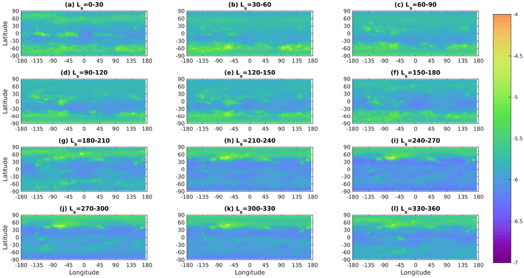
Mean spatial distribution at 5° × 5° resolution of GW activity expressed as log10 (K2 K−2) and derived from nightside off-nadir diagnoses for all MY 29–33 and the labeled periods. Black markers indicate where is less than 2.5 × . White space indicates that no data is available in the averaging bin.
Figure 14:
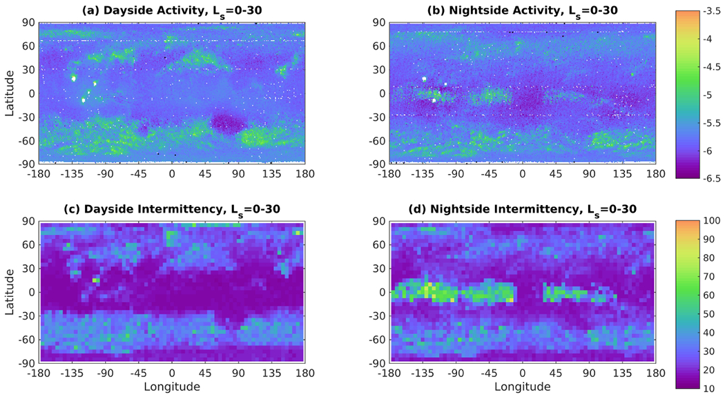
Mean spatial distribution of GW activity compared with intermittency for all available data during MY 29-33 and Ls = 0° — 30°. In panels (a) and (b), GW activity is expressed as log10 (K2 K−2) and derived from off-nadir diagnoses, with time-of-day as labeled. Resolution is 1° × 1°, black markers indicate where is less than 2.5 × , and white space indicates where no data is available in the averaging bin. In panels (c) and (d), intermittency (%) is plotted at a resolution of 5° × 5°, black markers indicate where is less than 2.5 × , and white space indicates where insufficient data is available in the averaging bin to estimate intermittency (n <10).
Figure 17:

Mean spatial distribution of GW activity compared with intermittency for all available data during MY 29–33 and Ls = 270° — 300°. In panels (a) and (b), GW activity is expressed as log10 (K2 K−2) and derived from off-nadir diagnoses, with time-of-day as labeled. Resolution is 1° × 1°, black markers indicate where is less than 2.5 , and white space indicates where no data is available in the averaging bin. In panels (c) and (d), intermittency (%) is plotted at a resolution of 5° × 5°, black markers indicate where is less than 2.5 , and white space indicates where insufficient data is available in the averaging bin to estimate intermittency (n <10).
First, mid-high latitude GW activity moves seasonally to follow the winter hemisphere. Activity is weakest at the summer pole and moderate at the winter pole (e.g., Figs. 12b–e,h–j; 13b–e,h–j). GW activity in the mid-latitudes tends to have similar seasonality. One example of this seasonal variability in GW activity is the hemispheric dichotomy border to the north of Arabia Terra. This area is a prominent region of activity from late northern summer to early northern spring (Figs. 12a,f–l) but not during the rest of the year, that is, most of northern spring and summer. When active, GW activity in this area has an intermittency around 40% (Fig. 14c). In northern spring and summer, GW activity is concentrated on Arabia and Sabaea themselves and relatively weak (Fig. 15a) with intermittency around 30%. A good example of this seasonal variability in the southern hemisphere is on the western side of Argyre. Dayside activity here is strongest in northern spring and summer (Figs. 12b–f; 15a) and pretty much absent in northern winter (e.g., Figs. 12k; 17a).
Figure 15:

Mean spatial distribution of GW activity compared with intermittency for all available data during MY 29-33 and Ls = 90° — 120°. In panels (a) and (b), GW activity is expressed as log10 (K2 K−2) and derived from off-nadir diagnoses, with time-of-day as labeled. Resolution is 1° × 1°, black markers indicate where is less than 2.5 × , and white space indicates where no data is available in the averaging bin. In panels (c) and (d), intermittency (%) is plotted at a resolution of 5° × 5°, black markers indicate where is less than 2.5 × , and white space indicates where insufficient data is available in the averaging bin to estimate intermittency (n <10).
Second, GW activity in the winter hemisphere tropics and the summer hemisphere is broadly weaker in northern fall and winter than northern spring and summer (Figs. 12d,j). At least in northern winter on the dayside, there seems to be a band of stronger GW activity in the southern tropics that does not have a strong analog in the northern tropics in the opposite season (Figs. 12h–k). Comparison at higher resolution (Figs. 15 and 17) broadly confirms this point and shows that the dayside northern winter activity is concentrated near the Tharsis Montes, around Syria and Sinai Plana, in Valles Marineris, and roughly on the opposite side of the planet (Fig. 17a). Typical intermittency in these areas is 30% except near topographic features such as the Tharsis Montes, where it it is as high as 60% (Fig. 17c). GW activity throughout the tropics and summer hemisphere is weaker on the nightside than the dayside (Figs. 12j, 13j). And areas of strong activity in the winter mid-latitudes are weaker on the nightside than the dayside. For example, when the boundary line of the hemispheric dichotomy to the north of Arabia Terra and Terra Sabaea can be seen on the dayside in Fig. 17a, it is barely discernible on the nightside (Fig. 17b).
Third, mountainous areas are persistent locations of strong GW activity, even though the highest surface elevations are excluded from the analysis. (Note the whitespace areas in the Tharsis Montes in Fig. 17a). This is clearest on the dayside, but many of these features are evident on the nightside as well. For example, in Fig 12a, the individual Tharsis Montes, Olympus Mons, Alba Patera, and Elysium are all discernible areas of activity, as are more obscure, low elevation features such as Acheron Fossae (38° N, 136 ° W) and the Phlegra Montes (40° N, 164 ° E). In addition, the ridges that surround Sinai and Solis Plana (surrounding 20 ° S, 100 ° W) are discernible areas of dayside GW activity throughout northern winter (Fig. 12h–k). They also are typically areas of higher intermittency (e.g. Fig. 17c). This phenomenon is partly under-resolution. An area where GW activity is associated with a topographic feature with a dimension much smaller than 5° will look like an area of high intermittency, because high variance only will be observed when the topographic feature is observed.
Fourth, the basins of the southern hemisphere (Hellas and Argyre) and the southern portions of the relatively smooth, low elevation plains of the northern hemisphere (Acidalia, Amazonis, and Arcadia Planitiae and parts of Vastitas Borealis) (Figs. 6b,d) are typically minima in GW activity on the dayside (e.g., Figs. 12h, 16a) and possibly minima in intermittency as well (Fig. 16c). However, areas of moderate GW activity are often observed on the southeastern and southwestern margins of the southern hemisphere basins, Argyre and Hellas (Fig. 16a).
Figure 16:

Mean spatial distribution of GW activity compared with intermittency for all available data during MY 29–33 and Ls = 180° – 210°. In panels (a) and (b), GW activity is expressed as log10 (K2 K−2) and derived from off-nadir diagnoses, with time-of-day as labeled. Resolution is 1° × 1°, black markers indicate where is less than , and white space indicates where no data is available in the averaging bin. In panels (c) and (d), intermittency (%) is plotted at a resolution of 5° Õ 5°, black markers indicate where is less than 2.5 , and white space indicates where insufficient data is available in the averaging bin to estimate intermittency (n <10).
Fifth, GW activity is sometimes high on the nightside in the tropics but not on the dayside. Such activity is sometimes observed near the Tharsis Montes but also can occur in other areas (e.g., Fig. 13a). However, the most persistent region of high, nightside-exclusive activity is centered in eastern Valles Marineris in the period from late northern winter to early northern fall (e.g., Figs. 13a–g,l). In early northern spring, there are three such areas at the Equator: (1) one stretching across Tharsis between Arsia and Pavonis Montes; (2) one over Valles Marineris centered on Eos Chasma; and (3) one in equatorial Terra Sabaea (Fig. 14b). Intermittency in these areas is 6080%, values generally associated with under-resolved topographic features but here extending over large areas (Fig. 14d). In early northern summer, there are two regions of GW activity associated with broad areas of high intermittency, one near Olympus Mons and one roughly centered on Ophir Planum (8° S, 58 ° W) (Fig. 15b,d). Inspection of the full seasonal cycle of nightside intermittency shows that areas of GW activity associated with high intermittency are common in northern spring and summer, particularly near the Tharsis Montes and eastern Valles Marineris (Figs. 18a–f). Note also that a nightside hotspot of activity near Eos Chasma (12° S, 40° W) was present during Ls =120°-150° in the off-nadir observations but not the nadir (Figs. 8b,d).
Figure 18:

Intermittency (%) of GW activity at 5° × 5° resolution derived from nightside off-nadir diagnoses for all sampled Mars Years and the labeled periods. White space indicates where insufficient data is available in the averaging bin to estimate intermittency (n <10)
To investigate the potential association between intermittent nightside GW activity in the tropics and CO2 ice clouds, features associated with optically thick clouds in A3 limb observations (Sefton-Nash et al., 2013) on the nightside between Ls =120°-150° of MY 29 were surveyed and ΩGW from off-nadir observations at the approximate latitude of these features in the same orbit was assessed. There is some subjectivity to this investigation, because these features can cover quite broad regions and merge with other features in the same orbit, making it a matter of judgment what variance corresponds to a feature. Our general rule was to select the peak variance that likely overlapped with a cloud feature.
Cloud features observed in the limb in A3 have a latitudinal and longitudinal distribution (Figs. 19a–b) that strongly resembles the spatial distribution of highly intermittent gravity wave activity observed on the nightside (Figs. 14b,d). However, 42% of cloud features are associated with variances typical of the background (ΩGW=0−0.1 K2, ). Nevertheless, other cloud features are associated with notable peaks in ΩGW as high as 8.53 K2 (Fig. 19c). Indeed, there are 315 instances of ΩGW > 0.5 K2 in the survey, but all are associated with a A3 cloud feature in the limb. Note also that there are only 64 instances of ΩGW > 0.5 K2 on the dayside during the survey period.
Figure 19:

Results from survey of optically thick cloud features in A3, Ls =120°–150° of MY 29 (n=491): (a) Latitudinal distribution of features; (b) Longitudinal distribution of features; (c) Distribution of ΩGW (K2), indicated both with a continuous trace and markers to show the discreteness of data
3.2.2. Interannual Variability
Global mean GW activity follows a repeatable seasonal cycle during the first half of the year. Dayside activity peaks at Ls = 30° and Ls = 150° and has a broad minimum around northern summer solstice. Nightside activity lacks the second maximum or has one of briefer duration (Fig. 20). During the second half of the year, most Mars Years have at least one intraseasonal decrease in global average GW activity (typically ≈ 10° of Ls) of 25-50% on both the dayside and nightside (Fig. 20). These decreases are most obvious during MY 31 at Ls = 210° and Ls = 315° and hardest to identify during MY 30 (Figs. 20c–d). A similar intraseasonal event appears to take place at Ls = 150° of MY 29, if the contrast between activity at this time and the typical maximum in activity is taken into account. Only during Ls = 190°-210° of MY 34 does mean nightside GW activity significantly exceed mean dayside activity, because of a substantial intraseasonal decrease in dayside activity synchronous with a substantial decrease in nightside activity (Fig. 20g).
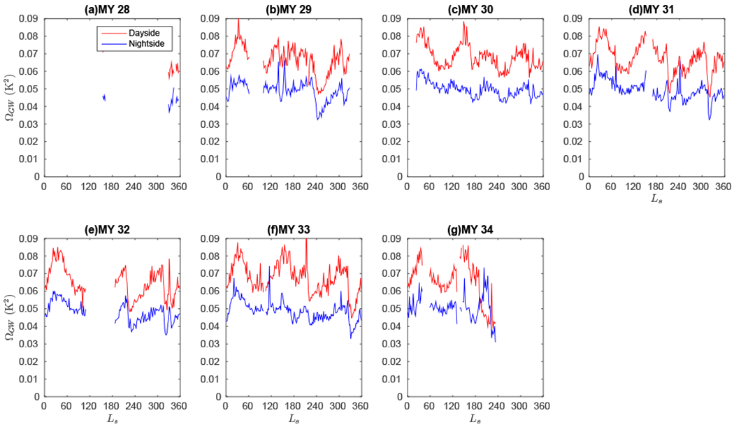
Figure 20:
Global mean based on off-nadir observations for the labeled Mars Years and time of day. Means of 2° Ls bins where there is no data, where is less than 2.5 × , or where sampling of the planet based on availability of data in 2° latitude bins is less than 90% are not plotted.
GW activity is typically greater during the first half of the year than the second half of the year. This trend is easier to see in because of warmer temperatures when Mars is closer to the Sun during northern winter/southern summer (Fig. 20). However, it also can be discerned in ΩGW (Fig. 21).
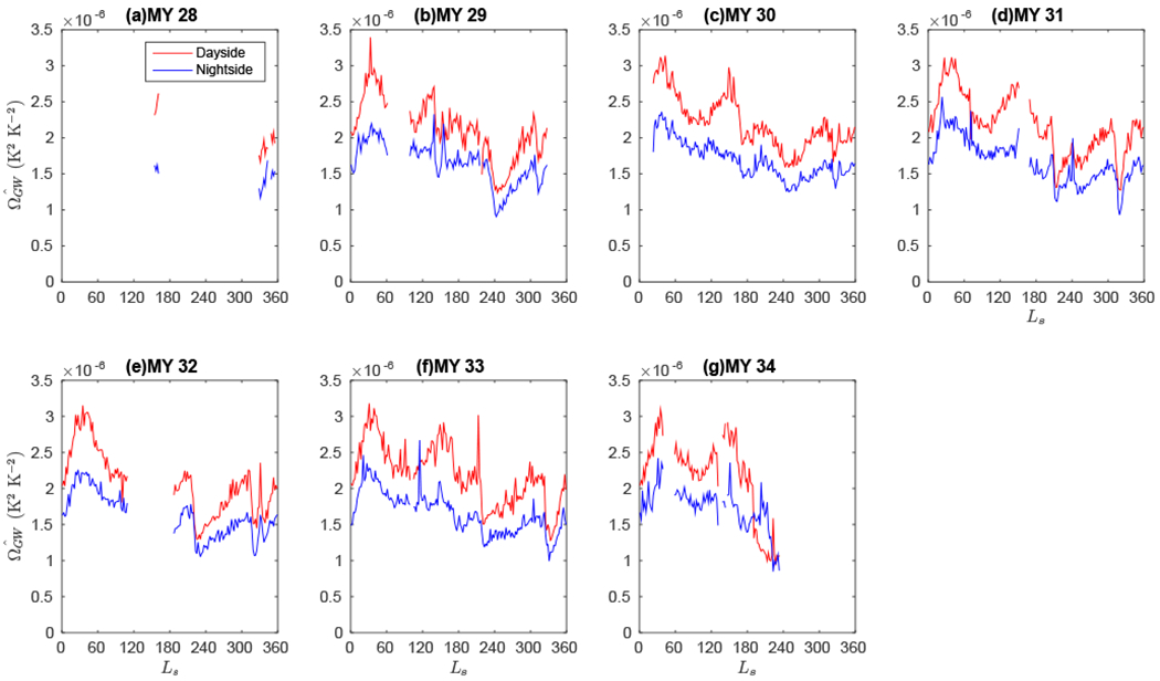
Figure 21:
Global mean ΩGW based on off-nadir observations for the labeled Mars Years and time of day. Means of 2° Ls bins where there is no data, where ΩGW is less than 2.5 × ∊GW, or where sampling of the planet based on availability of data in 2° latitude bins is less than 90% are not plotted.
The patterns that are seen in the seasonal means and global mean activity are visible in zonal mean GW activity as well. On the dayside in the tropics, activity is higher in the northern tropics during the first half of the year than the second half of the year (Fig. 22). The reverse is true for the southern tropics (Fig. 22). Activity at each pole peaks near winter solstice and is separated from the strongest zone of activity in the fall/winter mid-latitudes (Fig. 22). This zone is widest in latitude and centered most poleward at the equinoxes and narrows and moves equatorward toward winter solstice (Fig. 22).
Figure 22:

Zonal mean distribution vs. Ls of gravity activity expressed as log10 (K2 K−2) for the off-nadir dayside observations during the Mars Year labeled. Black markers indicate where is less than 2.5 . White space indicates that no data is available in the averaging bin.
In the second half of the year, there are occasional periods during which GW activity can be extremely low throughout the southern hemisphere and sometimes at higher latitudes, e.g., Ls = 240° during MY 29 or after Ls = 190° during MY 34 (Figs. 22a,f). These decreases coincide with the intraseasonal decreases in global mean GW activity (Fig. 20 and seem weakest during MY 30 (they do not penetrate the tropics) (Fig. 22b). In addition, there is a period of extremely low GW activity in the northern hemisphere at Ls = 150° of MY 29 (Fig. 22a).
On the nightside, the intraseasonal minima in GW activity and the extratropical variability are nearly identical to those on the dayside, except during MY 34, when northern mid-latitude GW activity increases after Ls = 190° to a level not seen in past years (Fig. 23). However, activity near the Equator during the first half of the year can be higher and more concentrated in latitude than on the dayside, particularly at Ls = 15° (Fig. 23). This contrast seems attributable to the large area of highly intermittent GW activity near the Equator during early northern spring (Fig. 14b,d).
Figure 23:

Zonal mean distribution vs. Ls of gravity activity expressed as log10 (K2 K−2) for the off-nadir nightside observations during the Mars Year labeled. Black markers indicate where is less than 2.5 × White space indicates that no data is available in the averaging bin.
Many of the intraseasonal minima coincide with well-known dust storms, such as the “early season activity”/regional dust storm around Ls = 150° of MY 29 (Smith, 2009; Wang and Richardson, 2015) (hereafter 29Z), the MY 29A regional dust storm around Ls = 240° of MY 29 (Kass et al., 2016) (hereafter 29A), and the MY 34 global dust event that started around Ls = 187° of MY 34 (hereafter 34P). This association is further established by the coincidence of these intraseasonal minima in GW activity with intraseasonal maxima in A3 dayside temperatures, particularly in the extratropics (Fig. 24). Intraseasonal maxima in temperature at this level of the atmosphere result from atmospheric heating by widespread hazes of dust and the dynamical response to this heating in regional and global dust storms (Kass et al., 2016). The effects of dust events on the spatial distribution of GW activity will be considered in the next section.
Figure 24:

Zonal mean dayside temperature in A3 off-nadir views calculated from during the Mars Year labeled (K). Black markers indicate where is less than 2.5 × . White space indicates that no data is available in the averaging bin.
3.3. GW Activity in Dust Storms
This analysis shows that dust storm activity substantially reduces GW activity in areas with climatologically low to moderate GW activity, particularly on the dayside. This effect can be seen in the regional dust storms, 29Z and 29A, when contrasting the spatial distributions of GW activity between the periods when these storms occurred and the following Mars Year (Figs. 25a–d and 26a–d). This effect is clearer when comparing GW activity during the MY 34 global dust event with a climatological average based on Mars Years without such a storm. Climatological areas of high activity in the northern mid-latitudes and high latitudes remain identifiable, while GW activity elsewhere is reduced by about an order of magnitude on the dayside and by a smaller amount at night, including in areas of high GW activity in the southern mid-latitudes (Figs. 27 and 28).
Figure 25:

Spatial distribution of global GW activity, log10 (K2 K −2) for the labeled periods and time of day. Resolution is 5° × 5°, black markers indicate where is less than 2.5 × , and white space indicates where no data is available in the averaging bin.
Figure 26:

Spatial distribution of global GW activity, log10 (K2 K−2) for the labeled periods and time of day. White space indicates areas without data. Resolution is 5° × 5°, black markers indicate where is less than 2.5 × , and white space indicates where no data is available in the averaging bin.
Figure 27:

Spatial distribution of global GW activity, log10 (K2 K −2) for the labeled periods and time of day. White space indicates areas without data. Resolution is 5° × 5°, black markers indicate where is less than 2.5 × , and white space indicates where no data is available in the averaging bin.
Figure 28:

Spatial distribution of global GW activity, log10 (K2 K −2) for the labeled periods and time of day. White space indicates areas without data. Resolution is 5° x 5°, black markers indicate where is less than 2.5 × , and white space indicates where no data is available in the averaging bin.
These reductions in GW activity and other changes developed along with the storm. On the dayside, a band of southern mid-latitude activity is discernible during the first few weeks of the storm and log10 was as low as ≈ −7 in a few areas (Figs. 27a–b). However, during the next periods, southern mid-latitude activity disappeared (but not in the climatology), and GW activity was extremely low over much of Mars’s tropics and southern mid-latitudes, except in a few areas such as Tharsis, just to the east of Tharsis, and near Syrtis Major (Figs. 27c–f). On the nightside, GW activity in the northern mid-latitudes was higher than normal in early stages of the storm, particularly in Arabia and Xanthe Terrae (30° N, 0° E) (Figs. 28a–b) but then strengthened to above climatological levels to the east and west (Figs. 28c–f).
Increased GW activity to the east of Tharsis reached climatologically unusual levels, though irregularly high GW activity of almost the same magnitude occurs around northern autumnal equinox in all sampled Mars Years (Figs. 29a–b). The strongest GW activity was concentrated near 5° N, 95 ° W at Ls = 205° (Fig. 29b). But similar magnitude activity occurred elsewhere in this region (Fig. 29c).
Figure 29:

GW activity in individual observations to (K2 K−2) to the east of the Tharsis Montes. (a) Time series of all observations in the labeled region/time-of-day of interest; (b) Time series of observations in MY 34 during the 2018 global dust event; (c) Individual observations during the labeled period plotted in map view. Magnitude of ΩGW is indicated by both marker size and color. The locations of Tharsis Tholus and Fortuna Fossae are indicated with “TT” and “FF” respectively.
Variance like that observed to the east of the Tharsis Montes during the MY 34 global dust event could suggest that strong, localized GW sources may be embedded within regional/global dust storms or indicate extremely large opacity variations at altitude (Appendix B). Both phenomena may be associated with deep convection (e.g., Spiga et al., 2013), for which the area east of the Tharsis Montes is a hotspot (Heavens et al., 2019).
Insight into whether dust storms can be GW sources comes from a fortuitous observation of a convective local dust storm over smooth terrain. A local dust storm was observed by MCS in NE Amazonis-SW Arcadia at Ls = 147.53 of MY 29 synchronous with the 29Z storm but away from its main area of dust haze (Heavens, 2017) (Fig. 30). Limb observations from MCS show that this storm mixed dust with mass mixing ratios of > 100 ppm well above the boundary layer to altitudes of 40 km (Heavens, 2017). The storm also cast a noticeable shadow (an indicator of its height) and had a “puffy” morphology that is thought to be indicative of deep convection (Strausberg et al., 2005; Kulowski et al., 2016) (Fig. 30a). In this season, GW activity is strong in the southern extratropics, where it was winter, but at the time when this dust storm was observed by visible imagery, activity of comparable magnitude was observed near 40° N (Fig. 30b). This activity peaks in the observations made by MCS directly over the optically thick dust clouds of the storm (Fig. 30a,c). Moreover, the two observations over the dust clouds observe the strongest GW activity by far in the dayside climatological record (n=2114) in this relatively topographically low and smooth area (Figs. 6b,d).
Figure 30:

Possible GW activity generated by a deep convective dust storm: (a) Visible image from the Mars Color Imager (MARCI) on board MRO (Wang and Richardson, 2015; Wang, cited 2016) with the location of diagnoses of GW activity from MCS off-nadir observations plotted with red crosses; (b) GW activity, (K2 K−2), observed on the dayside between Ls = 147.52 – 147.54 in MY 29; (c) The data in panel (b) for the area showed in panel (a); (d) Climatology of dayside GW activity, (K2 K−2), in the region 35°-40° N, 150°-155° W
And thus the storm would seem to be an unambiguous GW source; the amount of dust and temperature contrast with the gas opacity at 40 km are low enough to argue against the variance being explained by opacity variations alone. However, the vertical extent of the storm overlaps the A3 weighting function, so that the temperature variance could result from strong temperature variability within the dust cloud itself and might not necessarily have been caused by a GW.
4. Discussion
4.1. Comparison with Past Observations and Modeling
4-1.1. Observational Considerations
Nadir observations primarily sense meridionally propagating GW with horizontal wavelengths of 10-30 km with vertical wavelengths of greater than 50 km that are traveling near 25 km above the surface or near a pressure level of 50 Pa (Fig. 3a). Off-nadir observations primarily sense GW with a horizontal wavelength around 30 km and vertical wavelength of 10 km (Fig. 3b). Longer horizontal wavelengths may be sampled by nadir or off-nadir observations if the GW has some zonal orientation. The main agent of dissipation of these waves is likely to be trapping in the lowest part of the atmosphere by total internal reflection/ducting because of their short horizontal and long vertical wavelengths (Fritts and Alexander, 2003). If the atmosphere is considered to be a waveguide, the atmospheric properties and the intrinsic properties of the wave have to be such as to allow the waves to which the observations are sensitive to be admitted. In the approximation for high-frequency meridionally traveling waves with vertical wavelengths sufficiently less than 4πH (120 km for Mars) (Fritts and Alexander, 2003), the vertical wavelength, λz is restricted such that:
| (12) |
where c is the intrinsic horizontal phase velocity of the wave and v is the meridional wind.
Modeling suggests that dissipation of horizontal wavelengths longer than 30 km by ducting or shorter than 100 km by convective/shear instability is less likely for waves of this approximate vertical wavelength than longer waves (Kuroda et al., 2016; Imamura et al., 2016).
4.1.2. Comparison with Nadir Observations
The observations presented here are thus most comparable to past studies of GW activity from on-planet observations, which should share sensitivity to shorter horizontal wavelengths and longer vertical wavelengths. Imamura et al. (2007) calculated wavenumber power spectra of MGS-TES nadir observations near the center of the 15 micron CO2 band. The observations presented here are broadly consistent with the inference of Imamura et al. (2007) that GW activity at less than 200 km scales strongly contributes to the spectrum of wave energy in the winter extratropics (e.g., Figs. 15,17).
Also potentially comparable is the analysis of Altieri et al. (2012), which reports observations of potential GW oscillations in O2 dayglow between 55°-75° S around northern fall equinox. This area and season is indeed associated with substantial GW activity (Fig. 12f).
4.1.3. Comparison with Limb Observations
The observations presented here are less comparable with studies of GW activity that have considered the Ep in the lower atmosphere above the boundary layer short-wavelength temperature structures in radio occultation-based temperature retrievals (Creasey et al., 2006a; Tellmann et al., 2013). As noted above, this observational approach can be contaminated by tidal structures. Moreover, the observational geometry of this method likely gives a sensitivity analogous to that calculated in Figure 10 of Wu et al. (2006) for Global Positioning System (GPS) profiling of GW for horizontal wavelengths of 100-1000 km at vertical wavelengths of 1 km and for horizontal wavelengths of 300-1000 km at vertical wavelengths around 10 km. That said, these studies, consistent with the results presented here, generally find that the Tharsis Montes and other higher elevation areas have higher GW activity.
The observations presented here also are less comparable with those of Wright (2012), which considered GW activity inferred from MCS temperature retrievals from limb radiance observations. The methodology of Wright (2012) excluded vertical wavelengths of > 10 km to minimize tidal contributions and may undersample waves with horizontal wavelengths < 200 km and vertical wavelengths < 4-6 km. Indeed, the dominant horizontal wavenumber typically observed during northern fall and winter is 10−3 km−1 (equivalent to 6300 km, though this should be interpreted as an upper limit). These long wavelengths suggest that Wright (2012) mostly samples waves with very different horizontal length scales to the ones sampled by MRO-MCS on-planet views.
4.1.4. Comparison with Modeling
The seasonal cycle and spatial distribution of GW activity in the lower atmosphere has been considered by high resolution (67 km at the Equator or ≈ 1.1°) modeling by Kuroda et al. (2015, 2016, 2019), which would have resolved some of the GW observed by this study at higher latitudes. It is possible to extrapolate the observations (Appendix C) to estimate the spatial distribution of total GW energy per unit volume (Et) that would have been resolved by Kuroda et al. (2016) at the level observed by MCS off-nadir observations (1.5 pressure scale heights above the 260 Pa level shown by Kuroda et al. (2016) and 6.4 pressure scale heights below the 0.1 Pa level shown by Kuroda et al. (2016)) (Figs. 31a–b). This extrapolation helps identify the areas of observed GW activity significant for middle and upper atmospheric dynamics in comparison with what the model predicts. Such an approach to model comparison is possible because the shorter horizontal wavelength population dominates total wave energy at higher altitudes (Kuroda et al., 2016), so even if short horizontal wavelength GW activity is not associated with a spectrum of longer horizontal wavelength waves, total wave energy high in the middle and in the upper atmosphere will be nearly identical to the case in which a longer horizontal wavelength spectrum existed. Note that no corrections have been made for the observations sampling dominantly meridionally propagating waves and for dissipation with altitude, which would tend to lead to underestimate of the extrapolated Et.
Figure 31:

Total GW energy per unit volume (mJ m−3) in s=21-106 at 60 Pa extrapolated from the MY 29-MY 33 dayside and nightside averaged together for the labeled seasons (mJ m−3). White space indicates insufficient data in the average. Topography is marked in the black contours. See Appendix C for methodological details.)
Around southern summer solstice, the GCM of Kuroda et al. (2015, 2016, 2019) predicts the most dynamically important areas of GW are over southern Tharsis, Elysium (and to the west of Elysium), and a region centered at 45° N, 60° W. The observations suggest that 45° N, 60° W is a dynamically significant area of GW activity but so are 40° N, 40° E and the Phlegra Montes (Fig. 31a). GW activity is more localized to the highest Tharsis volcanoes (as opposed to the entire elevated region) in the observations than the GCM. Around northern fall equinox, the GCM predicts the most dynamically important areas of GW are over all of Tharsis, Elysium, and the north pole. The observations again suggest that 45° N, 60° W and 40° N, 40° E are areas of dynamically significant GW activity as well as an area near Lomonosov Crater (60° N, 5° W) (Fig. 31b). What GW activity is observed near Tharsis or Elysium is primarily restricted to the difficult to observe areas near the volcanoes. The inference to be drawn is that a consequence of the GCM underresolving GW at the scales to which the off-nadir observations are sensitive is to miss dynamically significant populations of GW in relatively localized, mid-high latitude areas.
In addition, the simulations of Kuroda et al. (2019) disagree somewhat with the seasonal cycle of GW activity observed here. GW activity (in terms of the temperature variance measured in this study) during southern hemisphere winter is simulated to be much weaker than in northern hemisphere winter (Kuroda et al., 2019). Yet observations suggest that they are similar in magnitude (Figs. 12a–l, 13a–l,22a–f; 23a–f).
Parameterizing GW activity from the simulations of Kuroda et al. (2016, 2019) still is superior to a more conventional topographic GW parameterization, because these simulations do capture that GW activity peaks in the extratropics during the winter. In contrast, the seasonality of GW activity predicted from wind stress is extremely weak (Fig. 32). This weak seasonality probably results from the dominance of surface roughness (Fig. 6c–d) on the wind stress calculation. The areas associated with the strongest wind stress are eastern Valles Marineris and Olympus Mons.
Figure 32:

log10 of the estimated meridional surface wind stress (Nm 2) averaged over all local times for the labeled seasons. Values less than 1 × 10⁻⁴ Nm−2 are plotted as 1 × 10⁻⁴ Nm−2
4.2. Interpretation
4.2.1. Source of GW in Nadir Observations
We propose that nadir observations primarily sample GW and mesoscale variability generated by boundary layer convection. This hypothesis would explain the three main characteristics of these waves: (1) strong diurnal variability in the tropics and northern mid-latitudes in the middle of northern summer; (2) the weak but significant correlation between elevation and GW activity in the tropics on the dayside and the moderate anti-correlation between GW activity and elevation on the nightside; (3) the absence of correlation between elevation and activity at night. It also could explain why GW activity observed in the off-nadir is generally higher and varies much less diurnally than that observed in the nadir.
Strong diurnal variability in GW activity would be expected to be driven by boundary layer convection in the parts of the planet subject to strongly variable diurnal heating of the surface, as should be true for the tropics and summer hemisphere except near the pole (where insolation is perpetual in summer), thus explaining the first characteristic of these waves. Second, the convective boundary layer height on Mars is strongly correlated with surface elevation, that is, convective boundary layer height is higher over higher elevations than lower elevations (Hinson et al., 2008; Hinson et al., 2019).
The difficulty is the expected wavelength of GW. Observations on the Earth suggest that the horizontal wavelengths of GW generated by boundary layer convection are typically 5-15 km (Kuettner et al., 1987), just overlapping the sensitivity of the nadir observations. And simulated wavelengths from Mars mesoscale simulations simulate horizontal wavelengths of 5 km (Spiga and Forget, 2009). The reason for this scale is partly understood theoretically. Boundary layers generate a wide spectrum of GW that are filtered at short horizontal wavelengths by trapping (Lane and Clark, 2002), the origin of the lower limit in horizontal wavenumber/upper limit in horizontal wavelength prior to filtering is explained by Lane and Clark (2002) as a “spatial modulation of the thermals”, which have a horizontal spacing of 2 km.
Because dry convective boundary layers can be much deeper on Mars than the Earth, we propose that the typical horizontal wavelength of GW generated by boundary layer convection can be larger as well, and thus convective boundary layers at higher surface elevations will generate GW to which MCS nadir observations are sensitive. On the Earth over land, thermals in two-dimensionally oriented convection (convective rolls) have spacing that scales with the convective boundary layer height, h such that roll spacing is ≈ 3h (Young et al., 2002). This scaling agrees well with the horizontal dimension of open cellular convection (≈ 5 km) simulated in Gusev Crater (with h = 1.5 km) by Spiga and Forget (2009), though horizontal thermal spacing in Lane and Clark (2002) appears to scale with h. Ao et al. (2012) finds a mean h over the Sahara (the global maximum) of 4 km at 17:00 LST, while Hinson et al. (2008) reports observations near 17:00 LST of convective boundary layer height in the tropics of Mars ranging from h =2.6-10 km. In some cases, the boundary layers over the highest surface elevations may be sufficiently high to contribute to nadir observations, introducing variability that may not be GW but thermal contrasts between the ascending and descending branches of convection cells. Recent idealized simulations of GW generated by heating within the boundary layer of Mars by Imamura et al. (2016), suggest that GW generated by boundary layer convection on Mars would have horizontal wavelengths of 10-50 km and vertical wavelengths of 10-20 km, which presumably could be stretched into the region of moderate simulated visibility to nadir observations (Fig. 3a) by strong meridional winds, following Eq. 12.
4.2.2. Sources of GW in Off-nadir Observations
Because of the shared range of sensitivity between the nadir and off-nadir (Fig. 3), boundary layer convection also contributes to GW activity observed by off-nadir observations. The importance of this source likely explains why GW activity in the tropics and summer hemisphere are stronger on the dayside than the nightside in off-nadir observations. However, other sources contribute, which fall into three main classes.
The first class of sources is associated with the winter pole. In the off-nadir, there is clear separation (at 75° S) between winter polar activity and mid-latitude activity (Fig. 22). This distinction is less clear in the north, but the seasonality of activity at both poles suggests there is a source of GW associated with the seasonal CO2 cap (Figs. 22–23). Pettengill and Ford (2000) argued that sloping, reflective clouds observed by MGS-MOLA during the winter over the north pole were CO2 clouds condensing in the presence of GW with horizontal wavelengths ranging from 5.4-64.8 km (as an upper limit) with vertical wavelengths of 4.0-13.2 km. Off-nadir observations would be able to sense the higher wavelength end of these GW (Fig. 3b). Further insight into the source is not possible from these observations. GW near the winter pole have little longitudinal variability and almost no intermittency (Figs. 15 and 17), perhaps implying that GW are strongly filtered in the lower atmosphere as happens over Antarctica during the summer (Hertzog et al., 2012).
The second class of sources are those that migrate with the main zonal jets, as modeled and inferred from observations (e.g., Forget et al., 1999; McCleese et al., 2010). In the mid-latitudes, these sources are strong in the fall and winter and absent in summer, following the winter westerly jet. In the tropics, association with a jet explains the contrast between GW activity being concentrated over northern Tharsis during northern summer and over southern Tharsis during southern summer (e.g., Fig. 12d,j), because the equatorial easterly jet shifts with the summer hemisphere (Forget et al., 1999). The contrast of mid-latitude GW activity with a wind stress-based prediction of GW activity (Fig. 32), particularly in northern hemisphere fall and winter would seem to preclude a dominantly topographic source.
However, analogy with the Earth suggests that the second class of sources are indeed topographic. The Earth-observing instruments with the most similar sensitivity to GW characteristics to MCS off-nadir: the Atmospheric Infrared Sounder (AIRS) onboard the NASA Aqua satellite and the Infrared Atmospheric Sounding Interferometer (IASI) onboard the European MetOp satellites observe peaks in GW activity in the winter mid-latitudes that contain hotspots of significant intermittency associated with small-scale topographic features such as the Andes, the Antarctic Mountains, Scandinavia, the Ural Mountains etc. (Hoffmann et al., 2014). Hotspots like these with moderate intermittency (at least relative to other areas of Mars) occur in our analysis, too, such as west of Argyre, Elysium, the Phlegra Montes, Alba Patera, N. Arabia, Kunowsky, Lyot, and Lomonosov craters. However, as noted by Hoffmann et al. (2017), the long vertical wavelength GW (> 20 km) to which AIRS is sensitive will be internally reflected near the surface except in conditions of strong unidirectional wind shear. Because topographic waves have zero intrinsic phase speed, Eq. 12 suggests that meridional wind speed over topography will need to be ≈ 13 ms−1 to allow propagation of GW with a vertical wavelength of 10 km and a horizontal wavelength of 30 km and ≈ 25 ms−1 to allow GW twice as long. Because AIRS and IASI observe cross-track, they are sensitive to both zonally and meridionally propagating waves. However, our analysis is mainly sensitive to meridionally propagating waves, and so GW activity is observed when meridional winds are strong enough to admit long vertical wavelengths and any GW activity excited by zonal winds is likely missed. Thus, the strong GW activity over Mars’s shield volcanoes may result from strong axially symmetric katabatic/anabatic circulations (Rafkin et al., 2002) that both excite GW and have a strong enough meridional wind component to enable them to be observed. And localized sources of high GW activity in the mid-high latitudes may indicate unusually strong meridional winds over topographic features as well (e.g., Acheron Fossae).
The third class of GW sources is that associated with highly intermittent nightside GW activity near the Equator (particularly in eastern Valles Marineris) during northern spring and summer and in the latest part of northern winter and earliest part of northern fall. One possible explanation could be GW excited by nighttime convection below radiatively cooling water ice clouds (Spiga et al., 2017). Convectively-generated GW are well-known on Earth. AIRS is sensitive to GW generated by moist convection (Hoffmann et al., 2014), which tend to propagate as concentric wavefronts (and thus with radial symmetry from their sources) (Holton and Alexander, 1999; Vadas et al., 2012) and would have non-zero phase speeds that could allow for their propagation even under light winds. However, observations of the thermal structures associated with this convection (Hinson and Wilson, 2004; Hinson et al., 2014; Wilson and Guzewich, 2014; Spigaet al., 2017) suggest that it is much more common near the Tharsis Montes than in eastern Valles Marineris. Another possible explanation could be orographic generation of GW by a strong, highly variable meridional wind system within Valles Marineris that is poorly resolved in global climate models. Valles Marineris is the roughest part of the planet (Fig. 6c–d) and thought to have complex mesoscale anabatic/katabatic wind systems (Toigo and Richardson, 2002; Inada et al., 2007; Spiga and Forget, 2009; Spiga, 2011). However, to confirm this, it would be necessary to conduct a full suite of mesoscale simulations throughout the tropics with realistic dust and aerosol to properly capture radiative balance, which is a critical control on the activity of these wind systems (Spiga, 2011), and this has yet to be done.
The association of the third source with probable CO2 ice clouds suggests a third explanation: that the source could be partially an artifact of high altitude opacity variations at the MCS observational scale. In that case, the presence of the source in off-nadir observations and its absence in nadir observations would result from the much larger opacity contribution enabled by the longer off-nadir path. The intermittency (interpreted as some clouds being associated with background variance and some being associated with very high variances) could be explained by variations in cloud properties. One possibility is that the high variances indicate freshly-formed clouds, which would be more opaque and horizontally smaller before being advected by primarily zonal winds, as in the interpretation of Vincendon et al. (2011). However, given that Vincendon et al. (2011) argues that the morphology of CO2 ice clouds stems from a genetic connection with GW, it is likely that GW partly contribute to the high variances. If the high variances result entirely from opacity variations, the maximum ΩGW observed in the CO2 ice cloud survey in Section 3.2.1 (8.53 K2) would correspond to Tabs in the off-nadir path of 0.16 and thus a nadir opacity at a wavelength of 4.3 μm of 0.54 (Appendix B). This explanation also would require that middle atmospheric CO2 ice clouds are significantly thicker/more frequent at night than during the day, as noted in the recent study of hazes in MCS observations by Clancy et al. (2019).
4.2.3. GW Activity in Regional/Global Dust Storms
Our results show that regional and global dust storms (1) reduce GW activity throughout most of the summer hemisphere and tropics, (2) enhance or do not significantly change GW activity in the winter mid-latitudes, and (3) can generate climatologically exceptional GW activity locally in the tropics or in topographically smooth areas of the mid-latitudes.
The likely mechanism for the first effect is the suppression of boundary layer convection underneath the dust lofted by the storm, which limits incoming solar radiation to the surface. The resulting enhancement in stability also decouples upper level winds from the surface while warming the atmosphere above the convective boundary layer. Surface winds, wind stress, and therefore potential topographic excitation of GW are all reduced (Pollack et al., 1979; Newman et al., 2002a,b), though gravity wave propagation in the lower atmosphere is presumably improved by higher stability (Fritts and Alexander, 2003).
This idea is supported by a variety of results. Only one third to one fourth of regional dust storms loft dust beyond the boundary layer to produce widespread dust hazes (Kass et al., 2016), but those that do are synchronous with large intraseasonal decreases in GW activity. For example, during MY 29, GW activity had large intraseasonal decreases around Ls = 150°,Ls = 240°, and Ls = 315°. Each of these events was associated with regional dust storm activity in visible imagery (Wang and Richardson, 2015) , warming of temperatures well above the boundary layer (Smith, 2009; Kass et al., 2016), and significant vertical transport of dust/water into the middle atmosphere (Heavens et al., 2011; Heavens et al., 2018). In contrast, during MY 30, Wang and Richardson (2015) identified 11 regional dust storms, but any intraseasonal decreases in GW activity during MY 30 were comparatively minor (Fig. 20b; Fig. 22b), as were effects on temperatures above the boundary layer outside the summer extratropics (Kass et al.,2016) and vertical dust/water transport into the middle atmosphere (Heavens et al., 2018). In addition, the decrease in dayside GW activity during the 34P global dust event and to a lesser extent, in the regional dust storms, 29Z and 29A, is mainly a decrease in areas of low to moderate GW activity away from the areas of high activity in the mid-latitudes associated with westerly jets. In other words, GW activity decreases in areas where boundary layer convection is interpreted to be a source of GW. Moreover, this effect became more widespread as the global storm developed and covered the whole planet with haze (Fig. 27).
The second effect also probably arises from the dust storm disturbing the mechanisms that generate GW under non-dust storm conditions, e.g., suppressing boundary layer convection. Differences in mid-latitude GW activity between regional and global dust storms and non-dust storm conditions likely result from circulation changes related to the dust storm, such as stronger, more unstable jets.
The third effect is harder to interpret, partly because of its intermittency and its moderate magnitude compared to GW activity interpreted to have topographic sources. (The magnitude of GW activity observed would be close to the mean on the dayside for this season over Olympus Mons, Tharsis Montes, and the Elysium Montes, and lower than the mean to the west of Argyre (Fig. 12e)). One possibility is that this climatologically exceptional activity arises from surface winds of extreme magnitude or unusual direction in the dust storm interacting with topography. This would explain the clustering of high variances during 34P observed near topographic features such as Fortuna Fossae (5° N, 93° W) and Tharsis Tholus (13° N, 91° W) (Fig. 29d). However, it would not explain high variances over extremely smooth terrain associated with the local dust storm in Amazonis-Arcadia during 29Z.
Another possibility is that these GW are generated by convection within the dust storm, which may have the correct wavelength characteristics to be observed by MCS on-planet views (Spiga et al., 2013; Imamura et al., 2016). The best argument for a convective GW source is the local dust storm in Amazonis-Arcadia during 29Z. This low elevation, smooth area experiences impressive local dust storms several times per Mars Year, but these storms (with the exception of the storm during 29Z) are organized around highly sheared shallow convection (Heavens, 2017). That the one deep convective storm known to have passed through the area produced a climatologically unusual GW signal but the other storms did not is highly suggestive (Fig. 30) but also could be explained by strong temperature variability within the dust cloud rather than a wave.
Thus, testing whether deep convection within dust storms is a GW source rigorously is difficult with the data investigated in this study. On Mars, the best-documented, directly-observed convective dust storms are those on Olympus and Arsia Montes during northern summer (Heavens et al., 2015, 2019), but diagnoses of ΩGW in these areas may be biased by surface contributions and may poorly contrast with the strong orographic wave generation by those mountains. Moreover, the altitudes to which convective updrafts are inferred to rise in regional and global storms (60-80 km) (e.g., Heavens et al., 2015; Heavens et al., 2018; Heavens et al., 2019) are well above the vertical range to which off-nadir observations are sensitive, suggesting that GW generated by a mechanical oscillator effect (e.g., Fritts and Alexander, 2003) would be missed by our analysis.
While the local dust storm in Amazonis-Arcadia during 29Z does not seem to have been dusty enough to generate significant re-emission in A3, the activity east of Tharsis during the MY 34 global dust event also could have been the result of high altitude opacity variations at 30 km scales minimally equivalent to > 300 ppm of dust (Appendix B), but the best explanation for such variability and any non-wave thermal variability would be organized convection at 30 km scales. So the variance signal in this case could be a mixture of GW, non-wave temperature variability, and opacity-related contributions in uncertain proportions.
5. Summary and Conclusion
In this study, we have presented the most comprehensive evaluation of GW activity of Mars’s lower atmosphere to date and have been able to robustly characterize its spatial variability, seasonal and interannual variability, and intermittency. In addition, unlike most prior studies that have considered the first two aspects of GW activity, the observational approach described here is sensitive to the part of the GW population most relevant for middle and upper atmospheric dynamics.
Three main conclusions can be drawn from the results. First, GW activity associated with topographic features is strong, moderately intermittent, and widespread on Mars. Important foci of activity include the volcanic peaks of Tharsis as well as craters in the mid-high latitudes of both the southern highlands and northern lowlands. Explicitly resolving GW in high resolution simulations seems to be a promising route to improved GW parameterization in global models, but this effort likely will benefit from additional observational constraints, particularly concerning source intermittency.
Second, the major source of interannual variability in GW activity is the occurrence and timing of regional and global dust storms. These storms reduce a background source of GW likely unconnected with topography, probably by suppressing boundary layer convection. But they also may enhance other sources by modifying the wind field and generating deep convection. The response of GW activity to the MY 34 global dust event mostly seems to be a more extreme case of effects observable in local and regional dust storm activity. This information will help better assess middle/upper atmospheric phenomena related to dust storm activity while adding a new dimension to the impact of dust storm activity on atmospheric escape processes (Imamura et al., 2016; Chaffin et al., 2017; Heavens et al., 2018).
Third, GW activity is a plausible explanation for strong, highly intermittent variances observed on the nightside tropics during Ls =330°-180°. And our observations provide further evidence that GW activity can be responsible for middle atmospheric CO2 ice cloud formation. In that case, GW generated by radiatively convective water ice clouds in the lower atmosphere could be the cause of middle atmospheric CO2 ice clouds, linking these two important types of clouds and mesoscale weather. However, it is also possible that these variances are partially generated by the CO2 ice clouds themselves, implying middle atmospheric CO2 ice clouds are significantly thicker/more frequent at night than during the day.
A wealth of GW information is likely hidden in any instrumental dataset that measures the radiance emitted by Mars’s atmosphere at high enough resolution and with enough density now and in the future. On-planet views in other MCS channels, MCS limb views, and MGS-TES nadir and limb views are natural targets. Studies from TES nadir and MCS on-planet views in other channels are likely to supplement the work done here, while limb views might be more sensitive to lower frequency waves, but both will have something interesting to see. The same point might be made about imaging data. Signatures of GW have been identified in visible imagery since the Viking era (e.g., Kahn, 1984; Inada et al., 2007) but remain little-studied. However, such information may contain hidden contributions from opacity and/or non-wave temperature variability, which motivates future observations of GW at Mars by techniques that can distinguish the clouds from GW and more confidently attribute variance to waves.
Acknowledgements
This work was supported by the NASA Mars Data Analysis, Solar System Workings, and Nexus for Exoplanet System Science programs (NNX14AM32G, NNX15AI33G, and NNX15AE05G). Work at the Jet Propulsion Laboratory, California Institute of Technology is performed under contract with NASA. We thank two anonymous reviewers for their helpful comments on the original version of this manuscript.
Appendix A. Evaluating the Surface Radiance Contribution in A3
We investigated the potential influence of surface radiance on the MCS A3 channel during approximately the same season and in the same high elevation areas investigated by Wilson and Richardson (2000). The position of each A3 detector relative to the position of the scene given by the RDR was computed by re-projecting the MCS detector array in Cartesian space along the orbital track of the spacecraft, taking account of crossing the anti-prime meridian. Elevation data was based on each A3 detector position and the MOLA 16 point per degree (ppd) elevation map archived on PDS.
Fig. A.1 suggests that 12 km surface elevation is a reasonable empirical criterion to distinguish high altitude areas that introduce significant bias to A3 channel brightness temperatures from low altitude areas where this effect is minor or absent. In addition, off-nadir observations appear to be more weakly affected by this bias than nadir observations. In nadir observations, there is a weak positive linear dependence of brightness temperature upon elevation up to approximately 12 km surface elevation, where there is a significant change of slope (Fig. A.1a), such that A3 brightness temperatures near the summit of Olympus Mons (surface elevation > 20 km) can be 40 K warmer than low elevation areas in the same season. Off-nadir observations are cooler and do not increase with elevation up to approximately 12 km surface elevation, where there are some instances of a positive relationship between brightness temperature and surface elevation that usually has a smaller slope than in nadir observations (Fig. A.1b).
Appendix B. Sensitivity of A3 Radiance Variance To High Altitude Aerosol Opacity
In this section, the apparent variance in A3 that can be generated by high altitude aerosol is estimated. Suppose the A3 channel detectors observe where brightness temperature would be some uniform temperature, . And there is no slope in across the detector because of geometry or any other factor such that detrending only requires removing a mean brightness temperature, . Re-emission of radiation emitted by aerosol at a higher altitude and contrasting temperature in the path of M > J > 0 detectors results in the brightness temperature in these detectors being . In this case:
| (B.1) |
By defining the difference between and Ťb as δTb Assuming a = 0 and –b = , Eq. 5 can be applied to write the potential opacity-generated variance as a function of the difference between and Ťb, δTb:
| (B.2) |
where the term dependent on M and J shall be called G(M, J) for purposes of reference.
The gas is sufficiently opaque in A3 in the lower atmosphere that it can be treated as a perfect emitter, such that δTb is approximately:
| (B.3) |
where B(T) is the Planck function, Tabs is the absorbing optical depth of the high altitude aerosol, is the effective air temperature at the level of CO2 gas emission, and is the effective air temperature at the level of high altitude aerosol emission.
In that case, the Tabs necessary to produce a specific variance, , is:
| (B.4) |
Analysis of Eq. B.2 suggests that the optimal configuration for high altitude aerosol producing significant variance in the observation would be to be observed by about one-half of the detectors (Fig. B.1a). Let us consider two contrasts of interest between the approximate pressure level of CO2 gas emission in A3 (50 Pa) and higher altitudes. At the equinoxes, 50 Pa temperatures in the mid-latitudes are as low as 160 K but 2 Pa (50 km) temperatures are as high at 195 K. And at the same time at the Equator, 50 Pa temperatures are up to 190 K but 0.7 Pa (60 km) temperatures are 135 K (McCleese et al., 2010). These contrasts would require τabs of 0.025 and 0.04 respectively to generate a variance of 0.5 K2 (Fig. B.1b).
Dust opacities this high are unlikely, except perhaps in extreme conditions associated with dust storm activity near the Tharsis volcanoes (Heavens et al., 2015, 2019). Assuming uniform mixing of dust with a scale height of 9 km, the approximate total dust column opacity in A3 consistent with dust opacities above the respective altitudes for the two thermal contrast examples above would be 6.5 and 31 respectively, corresponding to visible opacities of 83 and 400, based on the assumed aerosol properties in the MCS retrievals (Heavens et al., 2011; Kleinböhl et al., 2011). The corresponding dust mass mixing ratios under the same assumptions would be 900-4500 ppm. And these opacities/mass mixing ratios are still unreasonably high at a longer off-nadir path length.
Water ice opacities this high are likewise unlikely. Water ice clouds of 9 km thickness whose bottom was at the altitude of our examples would have mass mixing ratios of 360 ppm and 1100 ppm (Heavens et al., 2010), an factor of 4-13 more than the water amount that would be expected at these altitudes even during the moistening of the middle atmosphere observed during global dust storms (up to 200 ppmv) (Fedorova et al., 2018; Heavens et al., 2018). However, longer off-nadir path length may enable water ice clouds formed in regions where water injection into the middle atmosphere by deep convective transport is particularly strong to generate water ice clouds with mass mixing ratios of 120 ppm, which could contribute substantially to A3 radiance variance.
CO2 ice clouds may form from a GW or tidal perturbation from the 135 K at 0.7 Pa mean temperature of the second case (the first case’s mean temperature at 2 Pa of 190 K would be too warm), and these clouds likely have properties that would help them generate significant variance in A3 on-planet observations by MCS. Vincendon et al. (2011) report observations of extended, east-west oriented, and cirrus-like CO2 ice clouds with an opacity in the 4.3 μm CO2 ice absorption band of ≈ 0.2. For an effective radius of 1 μm, the estimated extinction coefficient at 4.3 μm is 4.2 (Montmessin et al., 2007). The A3 channel does not fully resolve the 15 μm absorption band of CO2 ice and so the extinction coefficient for 1 μm CO2 ice is ≈ 0.5 and the single scattering albedo is 0.15, suggesting that τabs in A3 would be 0.02. In off-nadir observations, where path lengths would increase by ≈ 2.9, these clouds may generate significant variances in A3, particularly if their width in the north-south direction are 20-30 km, as Vincendon et al. (2011) reports.
Figure A.1:

The relationship between surface elevation and A3 channel brightness temperatures on the dayside within the region of 10° S – 30° N, 150°–100° W: (a) Nadir observations during Ls=135°–143° of MY 28; (b) Off-nadir observations during Ls=135°–143° of MY 30. In both panels, 12 km surface elevation is marked with a black vertical line and the number of individual measurements by a detector are noted in the title.
Figure B.1:

Contribution of high altitude aerosol opacity to variance in A3: (a) G(21, J); (b) log10 tabs equivalent to = 0.5 K2 as a function of T and T — T for M = 21 and J =11
Appendix C. Comparing the Spatial Distribution of Gravity Wave Activity with High Resolution Global Modeling
Kuroda et al. (2016) reports the spatial distribution of GW activity in terms of total GW energy at 260 Pa, that is, ρ(Ep + Ek). We estimate Ep from Eq. 7 (without correcting for visibility) and note that GW observed by the off-nadir are high enough frequency that Ek ≈ Ep. In that case, (Ep + Ek) is equal to 1.92 × 10⁵ J kg−1. This quantity is assumed to be conserved between the altitude the waves are observed and 260 Pa, which will be true in the absence of dissipation. In that case, ρ(Ep + Ek) for 260 Pa in the Mars Reference Atmosphere (Kliore, 1978) will be 1.29 × 10⁶ mJ m−3.
Kuroda et al. (2016) evaluate GW energy over all available vertical wavelengths and over horizontal wavelengths corresponding to s=21-106. This is equivalent to a horizontal wavelength range of 134-666 km at the Equator (as claimed by Kuroda et al. (2016)) that truncates at higher latitude, though may include longer or shorter wavelengths because of spectral leaking. We estimate the available vertical wavelength range to be 4-40 km (twice the vertical grid spacing near 260 Pa to one-half the minimum height of the vertical grid). To translate between GW energy at the scales calculated from the model and the observations, we approximate total energy as following a power law such that:
| (C.1) |
where P and Q are constants and kh, kz etc. denote the horizontal wavenumber range. The underlying principle is that the vertical wavelength spectrum follows the power law observed (Ando et al., 2012) and the horizontal wavelength spectrum follows the characteristic universal power law for the mesoscale (Tung and Orlando, 2003). Eq. C.1 then was evaluated analytically at any latitude for the wavelength range resolved by (Kuroda et al., 2016). Eq. C.1 was then convolved with the off-nadir visibility and evaluated numerically to determine the amount of energy that would be observed by off-nadir observations relative to that in s=21-106. The result is a factor that can be used to extrapolate the energy observed by off-nadir observations to the wavelengths resolved by the GCM. This factor ranges from 28.5 at the Equator to 1.92 near the poles and was multiplied by 2.55 × 10⁵ UGW mJ m−3 to obtain Et.
Footnotes
Data Availability
Mars Climate Sounder calibrated radiance products are available from the NASA Planetary Data System. The variance diagnoses, spatial and temporal averages of variance diagnoses, and visibility functions from this study are archived publicly on Mendeley (Heavens, 2019).
References
- Albers JR, Birner T, 2014. Vortex preconditioning due to planetary and gravity waves prior to sudden stratospheric warmings. J. Atmos. Sci. 71, 4028–4054. URL: https://doi.Org/10.1175/JAS-D-14-0026.1, doi: 10.1175/JAS-D-14-0026.1, arXiv: 10.1175/JAS-D-14-0026.1. [DOI] [Google Scholar]
- Altieri F, Spiga A, Zasova L, Bellucci G, Bibring JP, 2012. Gravity waves mapped by the OMEGA/MEX instrument through O2 dayglow at 1.27 μm: Data analysis and atmospheric modeling. J. Geophys. Res. 117, E00J08. doi: 10.1029/2012JE004065. [DOI] [Google Scholar]
- Ando H, Imamura T, Tsuda T, 2012. Vertical Wavenumber Spectra of Gravity Waves in the Martian Atmosphere Obtained from Mars Global Surveyor Radio Occultation Data. J. Atmos. Sci. 69, 2906–2912. [Google Scholar]
- Ao CO, Waliser DE, Chan SK, Li JL, Tian B, Xie F, Mannucci AJ, 2012. Planetary boundary layer heights from GPS radio occultation refractivity and humidity profiles. J. Geophys. Res. 117. doi: 10.1029/2012JD017598. [DOI] [Google Scholar]
- Bandfield JL, Wolff MJ, Smith MD, Schofield JT, McCleese DJ, 2013. Radiometric comparison of Mars Climate Sounder and Thermal Emission spectrometer measurements. Icarus 225, 28–39. doi: 10.1016/j.icarus.2013.03.007. [DOI] [Google Scholar]
- Barnes JR, 1990. Possible effects of breaking gravity waves on the circulation of the middle atmosphere of Mars. J. Geophys. Res. 95, 1401–1421. doi: 10.1029/JB095iB02p01401. [DOI] [Google Scholar]
- Chaffin MS, Deighan J, Schneider NM, Stewart AIF, 2017. Elevated atmospheric escape of atomic hydrogen from Mars induced by high-altitude water. Nature Geosci. 10, 174–178. doi: 10.1038/ngeo2887. [DOI] [Google Scholar]
- Chandran A, Rusch D, Palo S, Thomas G, Taylor M, 2009. Gravity wave observations in the summertime polar mesosphere from the Cloud Imaging and Particle Size (CIPS) experiment on the AIM spacecraft. J. Atmos. Solar-Terr. Phys. 71, 392–400. URL: http://www.sciencedirect.com/science/article/pii/S1364682608002745, doi: 10.1016/j.jastp.2008.09.041. global Perspectives on the Aeronomy of the Summer Mesopause Region. [DOI] [Google Scholar]
- Clancy RT, Sandor BJ, W.M J., Christensen PR., Smith MD., Pearl JC., Conrath BJ., Wilson RJ., 2000. An intercomparison of ground-based millimeter, MGS TES, and Viking atmospheric temperature measurements: Seasonal and interannual variability of temperatures and dust loading in the global Mars atmosphere. J. Geophys. Res. 105, 9553–9571. [Google Scholar]
- Clancy RT, Wolff MJ, Smith MD, Kleinböhl A, Cantor BA, Murchie SL, Toigo AD, Seelos K, Lefevre F, Montmessin F, Daerden F, Sandor BJ, 2019. The distribution, composition, and particle properties of Mars mesospheric aerosols: An analy sis of CRISM visible/near-IR limb spectra with context from nearcoincident MCS and MARCI observations. Icarus 328, 246–273. URL: http://www.sciencedirect.com/science/article/pii/S0019103518307851, doi: 10.1016/j.icarus.2019.03.025. [DOI] [Google Scholar]
- Conrath BJ, Pearl JC, Smith MD, Maguire W, Christensen PR, Dason S, Kaelberer MS, 2000. Mars Global Surveyor Thermal Emission Spectrometer observations: Atmospheric temperature during aerobraking and science phasing. J. Geophys. Res. 105, 9509–9519. doi: 10.1029/2000JE001095. [DOI] [Google Scholar]
- Creasey JE, Forbes JM, Hinson DP, 2006a. Global and seasonal distribution of gravity wave activity in Mars’ lower atmosphere derived from MGS radio occultation data. Geophys. Res. Lett. 33, L01803. doi: 10.1029/2005GL024037. [DOI] [Google Scholar]
- Creasey JE, Forbes JM, Keating GM, 2006b. Density variability at scales typical of gravity waves observed in Mars’ thermosphere by the MGS accelerometer. Geophys. Res. Lett. 33, L22814. doi: 10.1029/2006GL027583. [DOI] [Google Scholar]
- Dunkerton TJ, 1997. The role of gravity waves in the quasi-biennial oscillation. J. Geophys. Res. 102, 26053–26076. doi: 10.1029/96JD02999. [DOI] [Google Scholar]
- Ern M, Preusse P, Alexander MJ, Warner CD, 2004. Absolute values of gravity wave momentum flux derived from satellite data. J. Geophys. Res. 109, D20103. doi: 10.1029/2004JD004752. [DOI] [Google Scholar]
- Fedorova A, Bertaux JL, Betsis D, Montmessin F, Korablev O, Maltagliati L, Clarke J, 2018. Water vapor in the middle atmosphere of Mars during the 2007 global dust storm. Icarus 300, 440–457. URL: http://www.sciencedirect.com/science/article/pii/S001910351730218X, doi: 10.1016/j.icarus.2017.09.025. [DOI] [Google Scholar]
- Forget F, Hourdin F, Fournier R, Hourdin C, Talagrand O, Collins M, Lewis SR, Read PL, Huot JP, 1999. Improved general circulation models of the martian atmosphere from the surface to above 80 km. J. Geophys. Res. 104, 24155–24176. [Google Scholar]
- Fritts DC, Alexander MJ, 2003. Gravity Wave Dynamics in the Middle Atmosphere. Rev. Geophys. 41, 3571–3589. doi: 10.1029/2001RG000106.1003. [DOI] [Google Scholar]
- Fritts DC, Isler JR, Thomas GE, Andreassen 0, 1993. Wave breaking signatures in noctilucent clouds. Geophysical Research Letters 20, 2039–2042. doi: 10.1029/93GL01982. [DOI] [Google Scholar]
- Fritts DC, Tsuda T, Kato S, Sato T, Fukao S, 1988. Observational evidence of a saturated gravity wave spectrum in the troposphere and lower stratosphere. Journal of the Atmospheric Sciences 45, 1741–1759. URL: , doi:, arXiv:. [DOI] [Google Scholar]
- Fritts DC, Wang L, Tolson RH, 2006. Mean and gravity wave structures and variability in the Mars upper atmosphere inferred from Mars Global Surveyor and Mars Odyssey aerobraking densities. J. Geophys. Res. 111, A12304. doi: 10.1029/2006JA011897. [DOI] [Google Scholar]
- Gong J, Wu DL, Eckermann SD, 2012. Gravity wave variances and propagation derived from AIRS radiances. Atmos. Chem. Phys. 12, 1701–1720. URL: https://www.atmos-chem-phys.net/12/1701/2012/, doi: 10.5194/acp-12-1701-2012. [DOI] [Google Scholar]
- Hayne PO, Paige DA, Heavens NG, 2014. The role of snowfall in forming the seasonal ice caps of Mars: Models and constraints from the Mars Climate Sounder. Icarus 231, 122–130. doi: 10.1016/j.icarus.2013.10.020. [DOI] [Google Scholar]
- Hayne PO, Paige DA, Schofield JT, Kass DM, Kleinböhl A, Heavens NG, McCleese DJ, 2012. Carbon dioxide snow clouds on Mars: South polar winter observations by the Mars Climate Sounder. J. Geophys. Res. 117. doi: 10.1029/2011JE004040. [DOI] [Google Scholar]
- Heavens N, 2019. Brightness Temperature Variances from On-Planet Views in the A3 Channel by the Mars Climate Sounder. Mendeley URL: http://dx.doi.Org/10.17632/7mnfcvtf53.1, doi: 10.17632/7mnfcvtf53.1. [DOI] [Google Scholar]
- Heavens NG, 2017. Textured Dust Storm Activity in Northeast Amazonis Southwest Arcadia, Mars: Phenomenology and Dynamical Interpretation. J. Atmos. Sci. 74, 1011–1037. URL:https://doi.Org/10.1175/JAS-D-16-0211.1, doi: 10.1175/JAS-D-16-0211.1, arXiv: 10.1175/JAS-D-16-0211.1. [DOI] [PMC free article] [PubMed] [Google Scholar]
- Heavens NG, Benson JL, Kass DM, Kleinböhl A, Abdou WA, McCleese DJ, Richardson MI, Schofield JT, Shirley JH, Wolkenberg PM, 2010. Water ice clouds over the martian tropics during northern summer. Geophysical Research Letters 37 URL: https://agupubs.onlinelibrary.wiley.com/doi/abs/10.1029/2010GL044610, doi: 10.1029/2010GL044610, arXiv:https://agupubs.onlinelibrary.wiley.com/doi/pdf/10 [DOI] [Google Scholar]
- Heavens NG, Cantor BA, Hayne PO, Kass DM, Kleinböhl A, McCleese DJ, Piqueux S, Schofield JT, Shirley JH, 2015. Extreme detached dust layers near Martian volcanoes: Evidence for dust transport by mesoscale circulations forced by high topography. Geophys. Res. Lett. 42, 3730–3738. doi: 10.1002/2015GL064004. [DOI] [Google Scholar]
- Heavens NG, Kass DM, Shirley JH, Piqueux S, Cantor BA, 2019. An Observational Overview of Dusty Deep Convection in Martian Dust Storms. Journal of the Atmospheric Sciences 76, 3299–3326. doi: 10.1175/JAS-D-19-0042.1. [DOI] [PMC free article] [PubMed] [Google Scholar]
- Heavens NG, Kleinböhl A, Chaffin MS, Halekas JS, Kass DM, Hayne PO, McCleese DJ, Piqueux S, Shirley JH, Schofield JT, 2018. Hydrogen escape from Mars enhanced by deep convection in dust storms. Nature Astron. 2, 126–132. doi: 10.1038/s41550-017-0353-4. [DOI] [Google Scholar]
- Heavens NG, Richardson MI, Kleinböhl A, Kass DM, McCleese DJ, Abdou W, Benson JL, Schofield JT, Shirley JH, Wolkenberg PM, 2011. The vertical distribution of dust in the Martian atmosphere during northern spring and summer: Observations by the Mars Climate Sounder and analysis of zonal average vertical dust profiles. J. Geophys. Res. 116. doi: 10.1029/2010JE003691.E04003 [DOI] [Google Scholar]
- Henderson V, Sayfi E, 2007. Mars Climate Sounder reduced data record software interface specification NASA Planetary Data System. NASA, Washington, D.C: D-37297. [Google Scholar]
- Henderson V, Sayfi E, 2012. MRO MCS Reduced Data Records (RDR) Software Interface Specification Version 1.4. Available online at https://atmos.nmsu.edu/PDS/data/MROM_1104/DOCUMENT/DP_SIS.ASC. [Google Scholar]
- Hertzog A, Alexander MJ, Plougonven R, 2012. On the in-Termittency of gravity wave momentum flux in the stratosphere. Journal of the Atmospheric Sciences 69, 3433–3448. URL:https://doi.Org/10.1175/JAS-D-12-09.1, doi: 10.1175/JAS-D-12-09.1, arXiv: 10.1175/JAS-D-12-09.1. [DOI] [Google Scholar]
- Hinson D, Tyler D, Lewis S, Pätzold M, Tellmann S, Husasler B, Tyler G, 2019. The martian daytime convective boundary layer: Results from radio occultation measurements and a mesoscale model. Icarus 326, 105–122. URL: http://www.sciencedirect.com/science/article/pii/S0019103518304329, doi: 10.1016/j.icarus.2019.02.028. [DOI] [Google Scholar]
- Hinson DP, Asmar SW, Kahan DS, Akopian V, Haberle RM, Spiga A, Schofield JT, Kleinböhl A, Abdou WA, Lewis SR, Paik M, Maalouf SG, 2014. Initial results from radio occultation measurements with the Mars Reconnaissance Orbiter: A nocturnal mixed layer in the tropics and comparisons with polar profiles from the Mars Climate Sounder. Icarus 243, 91–103. doi: 10.1016/j.icarus.2014.09.019. [DOI] [Google Scholar]
- Hinson DP, Pätzold M, Tellmann S, Hausler B, Tyler GL, 2008. The depth of the convective boundary layer on Mars. Icarus 198, 57–66. doi: 10.1016/j.icarus.2008.07.003. [DOI] [Google Scholar]
- Hinson DP, Wilson RJ, 2004. Temperature inversions, thermal tides, and water ice clouds in the Martian tropics. J. Geophys. Res. 109, E01002. doi: 10.1029/2003JE002129. [DOI] [Google Scholar]
- Hoffmann L, Alexander MJ, Clerbaux C, Grimsdell AW, Meyer CI, Roβler T, Tournier B, 2014. Intercomparison of stratospheric gravity wave observations with AIRS and IASI. Atmos. Meas. Tech. 7, 4517–4537. URL: https://www.atmos-meas-tech.net/7/4517/2014/, doi: 10.5194/amt-7-4517-2014. [DOI] [Google Scholar]
- Hoffmann L, Spang R, Orr A, Alexander MJ, Holt LA, Stein O, 2017. A decadal satellite record of gravity wave activity in the lower stratosphere to study polar stratospheric cloud formation. Atmos. Chem. Phys. 17, 2901–2920. URL: https://www.atmos-chem-phys.net/17/2901/2017/, doi: 10.5194/acp-17-2901-2017. [DOI] [Google Scholar]
- Holton JR, 1982. The role of gravity wave induced drag and diffusion in the momentum budget of the mesosphere. J. Atmos. Sci. 39, 791–799. URL: , doi:, arXiv:. [DOI] [Google Scholar]
- Holton JR, Alexander MJ, 1999. Gravity waves in the mesosphere generated by tropospheric convection. Tellus B 51, 45–58. URL: https://onlinelibrary.wiley.Com/doi/abs/10.1034/j.1600-0889.1999.00005.x, doi: 10.1034/j.1600-0889.1999.00005.x, arXiv:https://onlinelibrary.wiley.com/doi/pdf/10 [DOI] [Google Scholar]
- Holton JR, Haynes PH, McIntyre ME, Douglass AR, Rood RB, Pfister L, 1995. Stratosphere-troposphere exchange. Rev. Geophys. 33, 403–439. URL: https://agupubs.onlinelibrary.wiley.com/doi/abs/10.1029/95RG02097, doi: 10.1029/95RG02097, arXiv:https://agupubs.onlinelibrary.wiley.com/doi/pdf/10.10 [DOI] [Google Scholar]
- Imamura T, Kawasaki Y, Fukuhara T, 2007. Mesoscale Spectra of Mars’s Atmosphere Derived from MGS TES Infrared Radiances. J. Atmos. Sci. 64, 1717–1726. URL: 10.1175/JAS3914.1.!, doi: 10.1175/JAS3914.1, arXiv: 10.1175/JAS3914.1. [DOI] [Google Scholar]
- Imamura T, Watanabe A, Maejima Y, 2016. Convective generation and vertical propagation of fast gravity waves on Mars: One-and two-dimensional modeling. Icarus 267, 51–63. doi: 10.1016/j.icarus.2015.12.005. [DOI] [Google Scholar]
- Inada A, Richardson MI, McConnochie TH, Strausberg MJ, Wang H, , Bell JF, 2007. High-resolution atmospheric observations by the Mars Odyssey Thermal Emission Imaging System. Icarus 192, 378–395. doi: 10.1016/j.icarus.2007.07.020. [DOI] [Google Scholar]
- Jaquin, Robert Frederick I, 1989. The Middle Martian Atmosphere Ph.D. thesis. Cornell University. [Google Scholar]
- Kahn R, 1984. The spatial and seasonal distribution of Martian clouds and some meteorological implications. J. Geophys. Res. 89, 6671–6688. doi: 10.1029/JA089iA08p06671. [DOI] [Google Scholar]
- Kass DM, Kleinböhl A, McCleese DJ, Schofield JT, Smith MD, 2016. Interannual similarity in the Martian atmosphere during the dust storm season. Geophys. Res. Lett. 43, 6111–6118. doi: 10.1029/2016GL068978. [DOI] [Google Scholar]
- Kleinböhl A, Schofield J, Kass D, Abdou W, Shirley J, McCleese D, 2010. Combined limb/nadir retrievals of atmospheric parameters from Mars Climate Sounder measurements, in: 38th COSPAR Scientific Assembly, p. 7. [Google Scholar]
- Kleinböhl A, Schofield JT, Abdou WA, Irwin PGJ, de Kok RJ, 2011. A single-scattering approximation for infrared radiative transfer in limb geometry in the Martian atmosphere. J. Quant. Spectrosc. Radiat. Transf. 112, 1568–1580. doi: 10.1016/j.jqsrt.2011.03.006. [DOI] [Google Scholar]
- Kleinböhl A, Schofield JT, Kass DM, Abdou WA, Backus CR, Sen B, Shirley JH, Lawson WG, Richardson MI, Taylor FW, Teanby NA, McCleese DJ, 2009. Mars Climate Sounder limb profile retrieval of atmospheric temperature, pressure, and dust and water ice opacity. J. Geophys. Res. 114. doi: 10.1029/2009JE003358.E10006. [DOI] [PMC free article] [PubMed] [Google Scholar]
- Kliore A (Ed.), 1978. The Mars Reference Atmosphere Jet Propulsion Laboratory, California Institute of Technology. [Google Scholar]
- Kuettner JP, Hildebrand PA, Clark TL, 1987. Convection waves: Observations of gravity wave systems over convectively active boundary layers. QJRMS 113, 445–467. doi: 10.1002/qj.49711347603. [DOI] [Google Scholar]
- Kulowski L, Wang H, Toigo AD, 2016. The seasonal and spatial distribution of textured dust storms observed by Mars Global Surveyor Mars Orbiter Camera. Adv. Space Res. , -URL: http://www.sciencedirect.com/science/article/pii/S0273117716306226, doi: 10.1016/j.asr.2016.10.028. in press. [DOI] [Google Scholar]
- Kuroda T, Medvedev AS, Hartogh P, Takahashi M, 2009. On forcing the winter polar warmings in the martian middle atmosphere during dust storms. J. Meteor. Soc. Japan Ser. II 87, 913–921. doi: 10.2151/jmsj.87.913. [DOI] [Google Scholar]
- Kuroda T, Medvedev AS, Yiğit E, Hartogh P, 2015. A global view of gravity waves in the Martian atmosphere inferred from a high-resolution general circulation model. Geophys. Res. Lett. 42, 9213–9222. doi: 10.1002/2015GL066332. [DOI] [Google Scholar]
- Kuroda T, Medvedev AS, Yiğit E, Hartogh P, 2016. Global distribution of gravity wave sources and fields in the martian atmosphere during equinox and solstice inferred from a high-resolution general circulation model. J. Atmos. Sci. 73, 4895–4909. URL: https://doi.Org/10.1175/JAS-D-16-0142.1, doi: 10.1175/JAS-D-16-0142.1, arXiv: 10.1175/JAS-D-16-0142.1. [DOI] [Google Scholar]
- Kuroda T, Yiit E, Medvedev AS, 2019. Annual cycle of gravity wave activity derived from a high-resolution martian general circulation model. Journal of Geophysical Research: Planets 124, 1618–1632. URL: https://agupubs.onlinelibrary.wiley.com/doi/abs/10.1029/2018JE005847, doi: 10.1029/2018JE005847, arXiv:https://agupubs.onlinelibrary.wiley.com/doi/pdf/10. [DOI] [Google Scholar]
- Lane TP, Clark TL, 2002. Gravity waves generated by the dry convective boundary layer: Two-dimensional scale selection and boundary-layer feedback. Quart. J. Roy. Meteor. Soc. 128, 1543–1570. URL: https://rmets.onlinelibrary.wiley.com/doi/abs/10.1002/qj.200212858308, doi: 10.1002/qj.200212858308, arXiv:https://rmets.onlinelibrary.wiley.com/doi/pdf/10. [DOI] [Google Scholar]
- Liou K, 2002. Chapter 7 - application of radiative transfer principles to remote sensing, in: An Introduction to Atmospheric Radiation. Aca demic Press; volume 84 of International Geophysics, pp. 348–441. URL: http://www.sciencedirect.com/science/article/pii/S0074614202800225, doi: 10.1016/S0074-6142(02)80022-5. [DOI] [Google Scholar]
- McCleese DJ, Heavens NG, Schofield JT, Abdou WA, Bandfield JL, Calcutt SB, Irwin PGJ, Kass DM, Kleinböhl A, Lewis SR, Paige DA, Read PL, Richardson MI, Shirley JH, Taylor FW, Teanby N, Zurek RW, 2010. Structure and dynamics of the Martian lower and middle atmosphere as observed by the Mars Climate Sounder: Seasonal variations in zonal mean temperature, dust, and water ice aerosols. J. Geophys. Res. 115. doi: 10.1029/2010JE003677.E12016. [DOI] [Google Scholar]
- McCleese DJ, Schofield JT, 2012. MRO MCS Reduced Data Records (RDR) Dataset Information. Available online at https://atmos.nmsu.edu/PDS/data/MROM_1104/CATALOG/DATASET.CAT. [Google Scholar]
- McCleese DJ, Schofield JT, Taylor FW, Abdou WA, Aharonson O , Banfield D, Calcutt SB, Heavens NG, Irwin PGJ, Kass DM, Kleinböhl A, Lawson WG, Leovy CB, Lewis SR, Paige DA, Read PL, Richardson MI, Teanby N, Zurek RW, 2008. Intense polar temperature inversion in the middle atmosphere on Mars. Nature Geosci. 1, 745–749. doi: 10.1038/ngeo332. [DOI] [Google Scholar]
- McCleese DJ, Schofield JT, Taylor FW, Calcutt SB, Foote MC, Kass DM, Leovy CB, Paige DA, Read PL, Zurek RW, 2007. Mars Climate Sounder: An investigation of thermal and water vapor structure, dust and condensate distributions in the atmosphere, and energy balance of the polar regions. J. Geophys. Res. 112. doi: 10.1029/2006JE002790.E05S06. [DOI] [Google Scholar]
- MCD, cited 2018 Mars climate database v5.3: The web interface; [Available online at http://www-mars.lmd.jussieu.fr/]. [Google Scholar]
- Medvedev AS, Yiğit E, 2012. Thermal effects of internal gravity waves in the Martian upper atmosphere. Geophys. Res. Lett. 39, L05201. doi: 10.1029/2012GL050852. [DOI] [Google Scholar]
- Medvedev AS, Yiğit E, Hartogh P, 2011a. Estimates of gravity wave drag on Mars: Indication of a possible lower thermospheric wind reversal. Icarus 211, 909–912. doi: 10.1016/j.icarus.2010.10.013. [DOI] [Google Scholar]
- Medvedev AS, Yiğit E, Hartogh P, Becker E, 2011b. Influence of gravity waves on the Martian atmosphere: General circulation modeling. J. Geophys. Res. 116, E10004. doi: 10.1029/2011JE003848. [DOI] [Google Scholar]
- Montmessin F, Gondet B, Bibring JP, Langevin Y, Drossart P, Forget F, Fouchet T, 2007. Hyperspectral imaging of convective CO2 ice clouds in the equatorial mesosphere of Mars. Journal of Geophysical Research: Planets 112 URL: https://agupubs.onlinelibrary.wiley.com/doi/abs/10.1029/2007JE002944, doi: 10.1029/2007JE002944, arXiv:https://agupubs.onlinelibrary.wiley.com/doi/pdf/10. [DOI] [Google Scholar]
- Nakajima H, Suzuki M, Yokota T, Sugita T, Itou Y, Kaji M, Araki N, Waragai K, Yamashita H, Kanzawa H, Sasano Y, 2002. Tangent height registration for the solar occultation satellite sensor ILAS: A new technique for Version 5.20 products. Journal of Geophysical Research: Atmospheres 107, ILS 12–1-ILS 12–11. URL: https://agupubs.onlinelibrary.wiley.com/doi/abs/10.1029/2001JD000607, doi: 10.1029/2001JD000607, arXiv:https://agupubs.onlinelibrary.wiley.com/doi/pdf/10 [DOI] [Google Scholar]
- Newman CE, Lewis SR, Read PL, Forget F, 2002a. Modeling the Martian dust cycle, 1. Representations of dust transport processes. J. Geophys. Res. 107, 5123. doi: 10.1029/2002JE001910. [DOI] [Google Scholar]
- Newman CE, Lewis SR, Read PL, Forget F, 2002b. Modeling the Martian dust cycle 2. Multiannual radiatively active dust transport simulations. J. Geophys. Res. 107, 5124. doi: 10.1029/2002JE001920. [DOI] [Google Scholar]
- Parish HF, Schubert G, Hickey MP, Walterscheid RL, 2009. Propa gation of tropospheric gravity waves into the upper atmosphere of Mars. Icarus 203, 28–37. doi: 10.1016/j.icarus.2009.04.031. [DOI] [Google Scholar]
- Pettengill GH, Ford PG, 2000. Winter clouds over the north martian polar cap. Geophys. Res. Lett. 27, 609–612. doi: 10.1029/1999GL010896. [DOI] [Google Scholar]
- Piqueux S, Byrne S, Kieffer HH, Titus T, Hansen CJ, 2015. Enumeration of Mars years and seasons since the beginning of telescopic exploration. Icarus 251, 332–338. doi: 10.1016/j.icarus.2014.12.014. [DOI] [Google Scholar]
- Pollack JB, Colburn DS, Flasar FM, Kahn R, Carlston CE, Pidek DG, 1979. Properties and effects of dust particles suspended in the Martian atmosphere. J. Geophys. Res. 84, 2929–2945. doi: 10.1029/JB084iB06p02929. [DOI] [Google Scholar]
- Rafkin SCR, Sta. Maria MRV., Michaels TI., 2002. Simulation of the atmospheric thermal circulation of a martian volcano using a mesoscale numerical model. Nature 419, 697–699. doi: 10.1038/nature01114. [DOI] [PubMed] [Google Scholar]
- Sefton-Nash E, Teanby N, Montabone L, Irwin P, Hurley J, Calcutt S, 2013. Climatology and first-order composition estimates of mesospheric clouds from Mars Climate Sounder limb spectra. Icarus 222, 342–356. URL: [Google Scholar]
- Slipski M, Jakosky BM, Benna M, Elrod M, Mahaffy P, Kass D, Stone S, Yelle R, 2018. Variability of martian turbopause altitudes. Journal of Geophysical Research: Planets 123, 2939–2957. URL: https://agupubs.onlinelibrary.wiley.com/doi/abs/10.1029/2018JE005704, doi: 10.1029/2018JE005704, arXiv:https://agupubs.onlinelibrary.wiley.com/doi/pdf/10. [DOI] [Google Scholar]
- Smith MD, 2004. Interannual variability in TES observations of Mars during 1999–2003. Icarus 167, 148–165. doi: 10.1016/j.icarus.2003.09.010. [DOI] [Google Scholar]
- Smith MD, 2009. THEMIS observations of Mars aerosol optical depth from 20022008. Icarus 202, 444–452. doi: 10.1016/j.icarus.2009.03.027. [DOI] [Google Scholar]
- Spiga A, 2011. Elements of comparison between Martian and terrestrial mesoscale meteorological phenomena: Katabatic winds and boundary layer convection. Plan. Space Sci. 59, 915–922. doi: 10.1016/j.pss.2010.04.025. [DOI] [Google Scholar]
- Spiga A, Faure J, Madeleine JB, Manttanen A, Forget F, 2013. Rocket dust storms and detached dust layers in the Martian atmosphere. J. Geophys. Res. 118, 746–767. doi: 10.1002/jgre.20046. [DOI] [Google Scholar]
- Spiga A, Forget F, 2009. A new model to simulate the Martian mesoscale and microscale atmospheric circulation: Validation and first results. J. Geophys. Res. 114, E02009. doi: 10.1029/2008JE003242. [DOI] [Google Scholar]
- Spiga A, González-Galindo F, López-Valverde MA, Forget F, 2012. Gravity waves, cold pockets and CO2 clouds in the Martian mesosphere. Geophys. Res. Lett. 39, L02201. doi: 10.1029/2011GL050343. [DOI] [Google Scholar]
- Spiga A, Hinson DP, Madeleine JB, Navarro T, Millour E, Forget F, Montmessin F, 2017. Snow precipitation on Mars driven by cloud-induced night-time convection. Nature Geoscience 10, 652–657. doi: 10.1038/ngeo3008. [DOI] [Google Scholar]
- Strausberg MJ, Wang H, Richardson MI, Ewald SP, Toigo AD, 2005. Observations of the initiation and evolution of the 2001 Mars global dust storm. J. Geophys. Res. 110. doi: 10.1029/2004JE002361.E02006 [DOI] [Google Scholar]
- Tellmann S, Pätzold M, Hausler B, Hinson DP, Tyler GL, 2013. The structure of Mars lower atmosphere from Mars Express Radio Science (MaRS) occultation measurements. J. Geophys. Res. 118, 306–320. doi: 10.1002/jgre.20058. [DOI] [Google Scholar]
- Toigo AD, Richardson MI, 2002. A mesoscale model for the Martian atmosphere. J. Geophys. Res. 107, 5049. doi: 10.1029/2000JE001489. [DOI] [Google Scholar]
- Tolson R, Dwyer AM, Escalera PE, George BE, Hanna JL, Keating GM, Werner MR, 2005. Application of Accelerometer Data to Mars Odyssey Aerobraking and Atmospheric Modeling. J. Spacecraft Rockets 42, 435–443. doi: 10.2514/1.15173. [DOI] [Google Scholar]
- Tung KK, Orlando WW, 2003. The k3 and k5/3 energy spectrum of atmospheric turbulence: Quasigeostrophic two-level model simulation. Journal of the Atmospheric Sciences 60, 824–835. URL: , doi:, arXiv:. [DOI] [Google Scholar]
- Vadas S, Yue J, Nakamura T, 2012. Mesospheric concen tric gravity waves generated by multiple convective storms over the North American Great Plain. J. Geophys. Res. 117 URL: https://agupubs.onlinelibrary.wiley.com/doi/abs/10.1029/2011JD017025, doi: 10.1029/2011JD017025, arXiv:https://agupubs.onlinelibrary.wiley.com/doi/pdf/10 [DOI] [Google Scholar]
- Vincendon M, Pilorget C, Gondet B, Murchie S, Bibring JP, 2011. New near-IR observations of mesospheric CO2 and H2O clouds on Mars. Journal of Geophysical Research: Planets 116 URL: https://agupubs.onlinelibrary.wiley.com/doi/abs/10.1029/2011JE003827, doi: 10.1029/2011JE003827. [DOI] [Google Scholar]
- Walterscheid RL, Hickey MP, Schubert G, 2013. Wave heating and Jeans escape in the Martian upper atmosphere. Journal of Geophysical Research (Planets) 118, 2413–2422. doi: 10.1002/jgre.20164. [DOI] [Google Scholar]
- Wang H, cited 2016 Mars Daily Global Map Archive. URL: https://www.cfa.harvard.edu/hwang/mdgm/marci/.
- Wang H, Richardson MI, 2015. The origin, evolution, and trajectory of large dust storms on Mars during Mars Years 24–30 (1999–2011). Icarus 251, 112–127. doi:doi: 10.1016/j.icarus.2013.10.033. [DOI] [Google Scholar]
- Wilson RJ, 1997. A general circulation model of the Martian polar warming. Geophys. Res. Lett. 24, 123–126. doi: 10.1029/1996GL03814. [DOI] [Google Scholar]
- Wilson RJ, Guzewich SD, 2014. Influence of water ice clouds on nighttime tropical temperature structure as seen by the Mars Climate Sounder. Geophys. Res. Lett. 41, 3375–3381. doi: 10.1002/2014GL060086. [DOI] [Google Scholar]
- Wilson RJ, Lewis SR, Montabone L, Smith MD, 2008. Influence of water ice clouds on Martian tropical atmospheric temperatures. Geophys. Res. Lett. 35, L07202. doi: 10.1029/2007GL032405. [DOI] [Google Scholar]
- Wilson RJ, Richardson MI, 2000. The Martian atmosphere during the Viking mission. I. Infrared measurements of atmospheric temperatures revisited. Icarus 145, 555–579. doi: 10.1006/icar.2000.6378. [DOI] [Google Scholar]
- Withers P, 2006. Mars Global Surveyor and Mars Odyssey Accelerometer observations of the Martian upper atmosphere during aerobraking. Geophys. Res. Lett. 33, L02201. doi: 10.1029/2005GL024447. [DOI] [Google Scholar]
- Wright CJ, 2012. A one-year seasonal analysis of martian gravity waves using MCS data. Icarus 219, 274–282. doi: 10.1016/j.icarus.2012.03.004. [DOI] [Google Scholar]
- Wright CJ, Osprey SM,Gille JC, 2013. Global observations of gravity wave intermittency and its impact on the observed momentum flux morphology. Journal of Geophysical Research: Atmospheres 118, 10,980–10,993. URL: https://agupubs.onlinelibrary.wiley.com/doi/abs/10.1002/jgrd.50869, doi: 10.1002/jgrd.50869, arXiv:https://agupubs.onlinelibrary.wiley.com/doi/pdf/10.10C [DOI] [Google Scholar]
- Wu DL, Eckermann SD, 2008. Global Gravity Wave Variances from Aura MLS: Characteristics and Interpretation. J. Atmos. Sci. 65, 3695–3718. URL: 10.1175/2008JAS2489.1.!, doi: 10.1175/2008JAS2489.1, arXiv: 10.1175/2008JAS2489.1. [DOI] [Google Scholar]
- Wu DL, Preusse P, Eckermann SD, Jiang JH, Juarez MDLT, Coy L, Wang DY, 2006. Remote sounding of atmospheric gravity waves with satellite limb and nadir techniques. Adv. Space. Res. 37, 2269–2277. doi: 10.1016/j.asr.2005.07.031. [DOI] [Google Scholar]
- Wu DL, Waters JW, 1996. Gravity-wave-scale temperature fluctuations seen by the UARS MLS. Geophys. Res. Lett. 23, 3289–3292. doi: 10.1029/96GL02924. [DOI] [Google Scholar]
- Yamanaka M, 1995. Homopause control by gravity wave breaking in the planetary atmospheres. Adv. Space. Res. 15, 47–50. URL: http://www.sciencedirect.com/science/article/pii/0273117794000637, doi: 10.1016/0273-1177(94)00063-7. [DOI] [Google Scholar]
- Yiğit E, Medvedev AS, 2015. Internal wave coupling processes in earth’s atmosphere. Advances in Space Research 55, 983–1003. URL: http://www.sciencedirect.com/science/article/pii/S0273117714007236, doi: 10.1016/j.asr.2014.11.020. [DOI] [Google Scholar]
- Yiğit E, Medvedev AS, Hartogh P, 2015. Gravity waves and high-altitude co2 ice cloud formation in the martian atmosphere. Geophysical Research Letters 42, 4294–4300. URL: https://agupubs.onlinelibrary.wiley.com/doi/abs/10.1002/2015GL064275, doi: 10.1002/2015GL064275, arXiv:https://agupubs.onlinelibrary.wiley.com/doi/pdf/10 [DOI] [Google Scholar]
- Yiğit E, Medvedev AS, Hartogh P, 2018. Influence of gravity waves on the climatology of high-altitude martian carbon dioxide ice clouds. Annales Geophysicae 36, 1631–1646. URL: https://www.ann-geophys.net/36/1631/2018/, doi: 10.5194/angeo-36-1631-2018. [DOI] [Google Scholar]
- Young GS, Kristovich DAR, Helmfelt MR, Foster RC, 2002. Rolls, Streets, Waves, and More: A Review of Quasi-Two-Dimensional Struc-tures in the Atmospheric Boundary Layer. Bull. Amer. Meteor. Soc. 83, 997–1001. doi: 10.1175/1520-0477(2002)083j0997:RSWAMA2.3.CQ;2. [DOI] [Google Scholar]