Latent Differential Equation with Moderators: Simulation and Application

Abstract

Latent Differential Equations (LDE) is an approach using differential equations to analyze time series data. Due to its recent development, some technique issues critical to performing an LDE model remain. This article provides solutions to some of these issues, and recommends a step-by-step procedure demonstrated on a set of empirical data, which models the interaction between ovarian hormone cycles and emotional eating. Results indicated that emotional eating is self-regulated. For instance, when people have more emotional eating behavior than normal, they will subsequently tend to decrease their emotional eating behavior. In addition, a sudden increase will produce a stronger tendency to decrease than a slow increase. We also found that emotional eating is coupled with the cycle of the ovarian hormone estradiol, and the peak of emotional eating occurs after the peak of estradiol. Self-reported average level of negative affect moderates the frequency of eating regulation and the coupling strength between eating and estradiol. Thus, people with a higher average level of negative affect tend to fluctuate faster in emotional eating, and their eating behavior is more strongly coupled with the hormone estradiol. Permutation tests on these empirical data supported the reliability of using LDE models to detect self-regulation and a coupling effect between two regulatory behaviors.

Introduction

The reality we inhabit is full of changes. In many cases a pattern of change can be detected that involves fluctuation around some equilibrium or “typical” value; examples include the swing of a pendulum in physics, the fluctuations of prices in economics, or the rise and fall of emotion in psychology. This type of change is frequently treated as error which is independently distributed around the equilibrium. However, observations in the time series often are not independent of each other. Our current state may depend on our previous state, and our upcoming state may, to some extent, be determined by our current state. One method to estimate the time-dependency information in the time series data is differential equation modeling.

In the quantitative psychology literature, several methods are used to describe change, such as multivariate analysis of variance (McCall & Appelbaum, 1973), hierarchical linear modeling (Raudenbush & Bryk, 2002), time series (Box, Jenkins, & Reinsel, 1970) and growth curve modeling (Duncan, Duncan, Strycker, Li, & Alpert, 1999). However, most of these methods are not designed to reveal fluctuations. Time series analysis¹ such as the autoregressive model is able to describe trajectories, but it cannot solve the phase problem (Boker & Nesselroade, 2002) as described below. The fluctuation of each individual is often not synchronized with other people. Individuals may have randomized phases: at any one moment, some may be at a peak, some may be in a valley, some may be increasing, some may be decreasing. So even though different individuals’ patterns of change might be the same, methods such as time series that estimate average trajectories frequently cannot detect it. The phase problem can be avoided by using differential equation modeling, which is defined as “expressing effects within a system in terms of the derivatives as well as in terms of the values of the variables themselves” (Boker & Graham, 1998, p. 481). Compared with methods describing trajectories, differential equation modeling examines the relationship between variables and their derivatives that are stable, regardless of phase.

There is a long history of using differential equations to describe the behavior of complex dynamical systems in physics, engineering, biomechanics and some social science areas (e.g., Hajek, 1968; Beltrami, 1987; Beek, Schmidt, Morris, Sim, & Turvey, 1995; Amazeen, Amazeen, & Turvey, 1998). In the recent decade, research in psychology applying differential equation modeling is growing quickly. This method has been used to study self-regulations in adolescent substance use (Boker & Graham, 1998), the well-being of recently bereaved older adult widows (Bisconti, Bergeman, & Boker, 2004), arm movements (Butner, Amazeen, & Mulvey, 2005), emotion regulation (Chow, Ram, Boker, Fujita, & Clore, 2005), resilience in adulthood and later life (Montpetit, Bergeman, Deboeck, Tiberio, & Boker, 2010; Ong, Bergeman, & Boker, 2009), violent behavior in psychiatric patients (Odgers et al., 2009), oscillations in daily pain prediction (Finan et al., 2010) and other longitudinal processes.

As a result of years of development, differential equation modeling is now becoming a mature longitudinal data analytic technique. However, some practical issues remain. The present article will show how to implement differential equation modeling in an SEM framework, i.e., latent differential equation (LDE, Boker, Neale, & Rausch, 2003), and solve the related technique issues. The article is organized in the following manner. First, background for LDE is introduced, including theory, terms, model and important parameters. Second, several related technique issues and our solutions are presented, and simulations are conducted to verify each solution. Then, a recommended LDE procedure is applied to a set of empirical data, which measures daily changes in eating behavior, hormone levels and negative affect.

Latent Differential Equations (LDE)

Second Order Differential Equations

Differential equations specify relationships between variables and their derivatives. Given a variable x, for example, positive affect, the first derivative ẋ expresses the velocity of change, which is the amount of change in positive affect per unit of time. The second derivative ẍ expresses the acceleration of change, which is the rate at which positive affect changes its velocity. A second order differential equation, in which the highest order of derivatives is 2, is sufficient to describe a damped linear oscillation. A linear oscillation stands for a system that has a restoring force that varies linearly with position. A damped linear oscillation adds some resistance to the linear oscillation thus energy will be drained from the system to overcome the resistive force. In a damped linear oscillatory system, we will see a periodic fluctuation around a central point (equilibrium) with the peaks or the amplitude of the fluctuation decreasing with time.

Equation 1 is a second order Differential equation representing a damped linear oscillation, where x is the displacement of a variable from its equilibrium, ẋ is the first derivative of the variable, ẍ is the second derivative of the variable, η is the regression coefficient of x on ẍ, and ζ is the regression coefficient of ẋ on ẍ.²

$$\ddot{x}=\eta x+\zeta \dot{x}+e$$ (1)

The parameters η and ζ have substantive meanings. The parameter η is called the frequency parameter, which mainly determines the frequency of the oscillation. In a self-regulation system, η is a negative number, indicating that when the system is away from its equilibrium, it will accelerate towards the equilibrium. If η is a positive number, no regulation occurs, since the system tends to accelerate father away when it leaves the equilibrium. The parameter ζ is called the damping parameter, which determines the amplitude of the oscillation. If ζ < 0, when ẋ is a positive number, that is the value of variable x is increasing with time, the person will tend to move in the opposite direction, that is to decrease the value of x, no matter whether the current location of x is above or below its equilibrium. So the oscillation would fade away with time if no outside force were to be working on it. In other words, the amplitude of the oscillation will decrease with time. If ζ = 0, whether x is increasing or decreasing will not influence one’s tendency. So the amplitude of the oscillation will be constant. And if ζ > 0, when x is increasing, one tends to accelerate the increase. As a result, the amplitude of the oscillation will increase with time. In fact, to form an oscillation requires that η < 0 and η + ζ²/4 < 0. The length of oscillating period in number of measures, λ (one over the frequency), can be calculated by Equation 2. Note that using differential equations to describe a dynamic system does not require that the system must be a self-regulation system with oscillations.

$$\lambda =\frac{2\pi }{\sqrt{-\left(\eta +{\zeta }^2/4\right)}}$$ (2)

Time Delay Embedding

One way to estimate derivatives (ẋ and ẍ) involves cutting time series data into short segments. Then, the derivatives at the middle point of each short segment can be estimated by local linear approximation (Boker & Graham, 1998), which uses a triplet of observations to estimate derivatives at the middle point. In this method, the interval between observations in the triplet is called the smoothing parameter τ. The value of τ determines the degree of smoothing. When τ is too large, it might smooth over the signal. If τ is too small, high frequency noise reduces the reliability of the signal. We could use this method to estimate derivatives. However, human behavior data includes a lot of noise and using only three observations to estimate derivatives becomes unreliable. More local observations should be considered in order to obtain a better estimation. We use a parameter D to denote the number of local observations used to estimate derivatives, and a parameter s to denote the time interval between two observations, which is predetermined by data. Thus (D − 1) × s is the length of the short segment used to estimate derivatives, which determines the degree of smoothing. In comparison, in the method using three observations to estimate derivatives, τ × 2 is the length of the time segment. Figure 1 shows a time series with three example segments estimating derivatives at T1, T2 and T3 respectively. The time segment D = 3 is the same length as the time segment τ = s, D = 5 is the same length as τ = 2s, and D = 7 is the same length as τ = 3s, but differently, our time segments include more than three observations. The setting of D is important to estimate differential equation models, and will be elaborated later.

Figure 1.

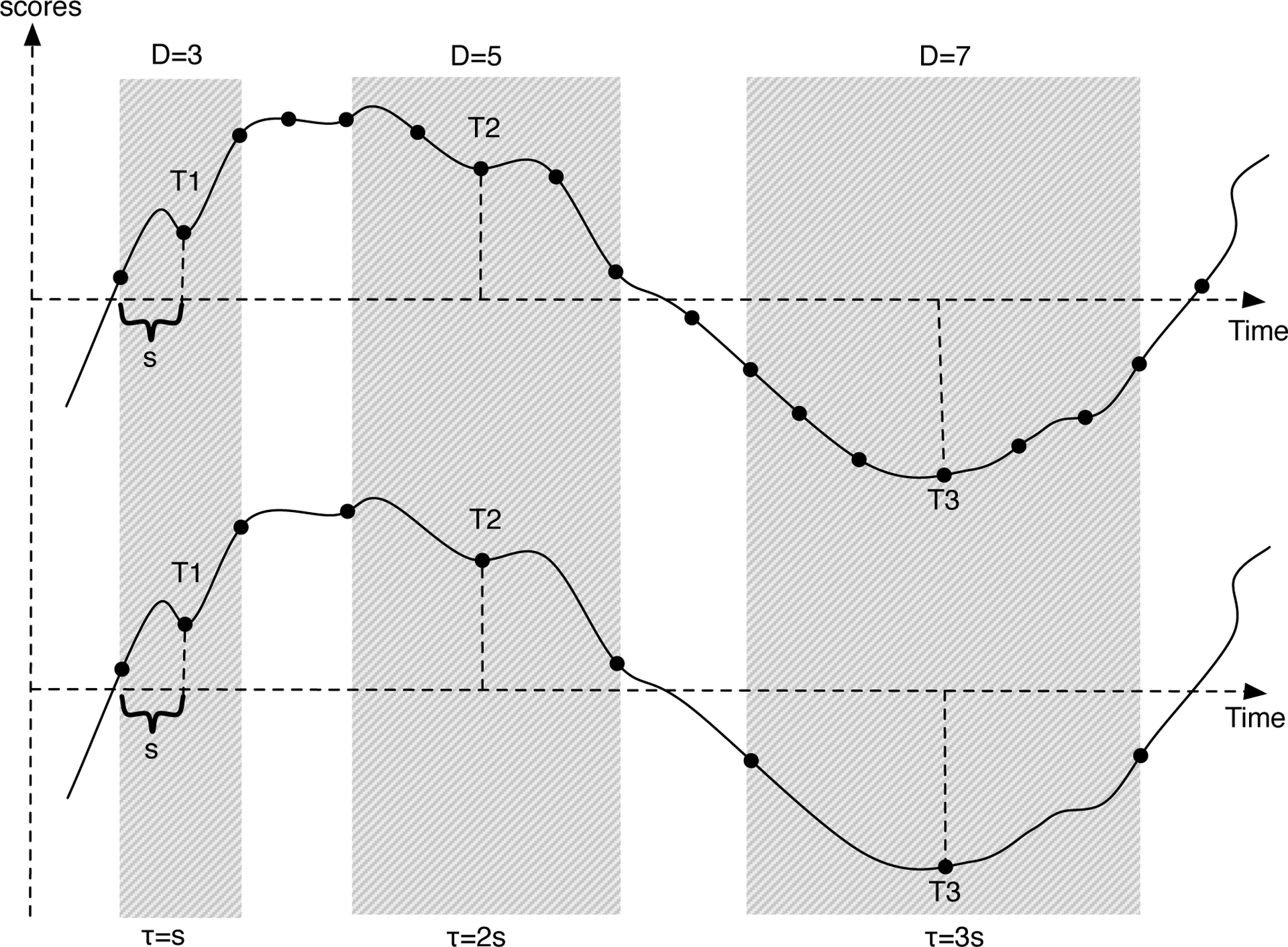
Illustration of the meaning of smoothing parameter D and τ.

Cutting time series into short segments can be implemented by constructing a time-delay embedding (Noakes, 1991), which uses overlapping samples to increase the precision of parameter estimation (Von Oertzen & Boker, 2010). Equation 3 is an example of a time-delay embedding data matrix for D = 5 segments. Please note that we use D = 5 here just for demonstration. The value of D does not necessarily need to be 5. We will show how to select the value of D later. The example matrix includes n persons with p observations each, where x_(i,j) stands for the observation obtained from person i at time j. Each row stands for a time segment including five observations. In standard terminology, we call this “a five dimensional time-delay embedding”.

$$X^{\left(5\right)}=\left[\begin{array}{ccccc}{x}_{(1,1)}& x_{(1,2)}& x_{(1,3)}& x_{(1,4)}& x_{(1,5)}\\ x_{(1,2)}& x_{(1,3)}& x_{(1,4)}& x_{(1,5)}& x_{(1,6)}\\ ⋮& ⋮& ⋮& ⋮& ⋮\\ x_{(1,p-4)}& x_{(1,p-3)}& x_{(1,p-2)}& x_{(1,p-1)}& x_{(1,p)}\\ x_{(2,1)}& x_{(2,2)}& x_{(2,3)}& x_{(2,4)}& x_{(2,5)}\\ ⋮& ⋮& ⋮& ⋮& ⋮\\ ⋮& ⋮& ⋮& ⋮& ⋮\\ x_{(n,1)}& x_{(n,2)}& x_{(n,3)}& x_{(n,4)}& x_{(n,5)}\\ x_{(n,2)}& x_{(n,3)}& x_{(n,4)}& x_{(n,5)}& x_{(n,6)}\\ ⋮& ⋮& ⋮& ⋮& ⋮\\ x_{(n,p-4)}& x_{(n,p-3)}& x_{(n,p-2)}& x_{(n,p-1)}& x_{(n,p)}\end{array}\right]$$ (3)

A time-delay embedding data set X⁽⁵⁾ can be used to estimate the first order and second order derivatives. Let Y be a matrix with 3 columns respectively representing the displacement (x), the first order derivative (ẋ) and the second order derivative (ẍ)

$$Y=\left[\begin{array}{ccc}{x}_{(1,3)}& {\dot{x}}_{(1,3)}& {\ddot{x}}_{(1,3)}\\ x_{(1,4)}& {\dot{x}}_{(1,4)}& {\ddot{x}}_{(1,4)}\\ ⋮& ⋮& ⋮\\ x_{(1,p-2)}& {\dot{x}}_{(1,p-2)}& {\ddot{x}}_{(1,p-2)}\\ x_{(2,3)}& {\dot{x}}_{(2,3)}& {\ddot{x}}_{(2,3)}\\ ⋮& ⋮& ⋮\\ x_{(n,3)}& {\dot{x}}_{(n,3)}& {\ddot{x}}_{(n,3)}\\ ⋮& ⋮& ⋮\\ x_{(n,p-2)}& {\dot{x}}_{(n,p-2)}& {\ddot{x}}_{(n,p-2)}\end{array}\right]$$

and L be the loading matrix

$$L=\left[\begin{array}{ccc}1& -2s\tau & {(-2s\tau )}^2/2\\ 1& -1s\tau & {(-1s\tau )}^2/2\\ 1& 0& 0\\ 1& 1s\tau & {(1s\tau )}^2/2\\ 1& 2s\tau & {(2s\tau )}^2/2\end{array}\right]$$

Then we model X⁽⁵⁾ as

$$X^{(5)}=Y{L}^T$$

where L^T is the transpose of the loading matrix L (Boker et al., 2003).

Structural Equation modeling of Differential Equations

Latent Differential Equation (LDE) uses structural equation modeling (SEM) to estimate differential equations. Specifically, the derivatives Y are treated as latent variables, and the dimensions of the time-delay embedded data X⁽⁵⁾ are treated as manifest variables. Figure 2 shows an LDE model using 5 dimensional time-delay embedded data, in which the loadings of the time-delay embedded data set on the derivatives are fixed to be the L matrix, and the relationship between derivatives (η and ζ) is estimated. With the time-delay embedded data X⁽⁵⁾ and the factor loadings L, one can estimate a differential equation as an ordinary SEM model. A reasonable concern is that the rows in the time-delay embedded data are not independent, which might result in alpha inflation. Counter to intuition, Von Oertzen and Boker (2010) demonstrated by mathematical derivation and simulation that instead of alpha inflation, using overlapping samples in this way can improve estimation and produce a smaller actual standard error in parameter estimation for linear second order differential equation models.

Figure 2.

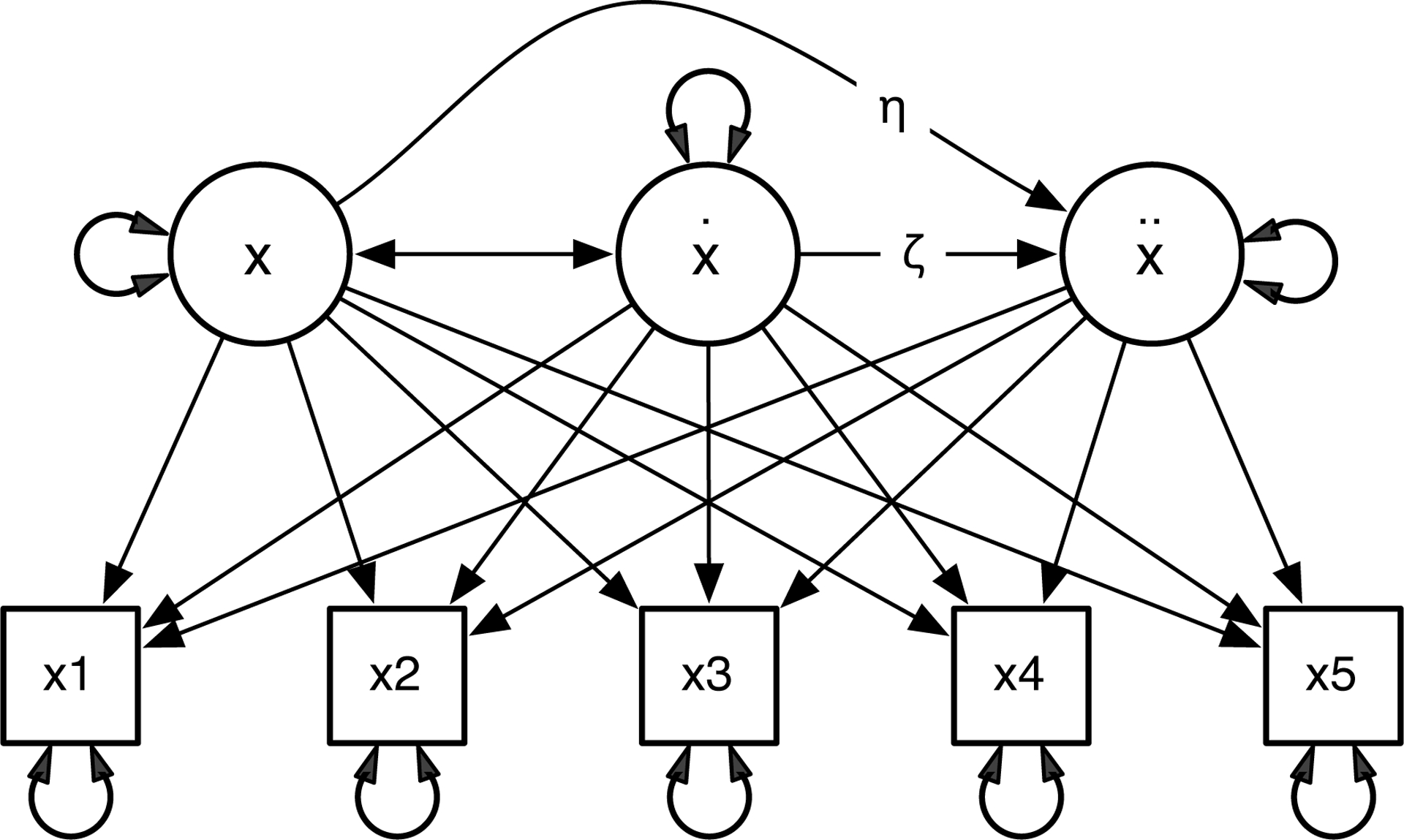
Single Latent Differential Equation Model (Single LDE).

LDE is also capable of estimating the relationship among several dynamic processes simultaneously. Figure 3 shows a coupled LDE model, which includes two single LDE models and the coupling effect between them. Besides the parameters η and ζ, the coupled LDE model has several coupling parameters γ. These parameters estimate the intrinsic regulation of each variable, as well as the extrinsic drive from the other variable in the same system. The substantive meanings of these coupling parameters may be obscure to many readers. We will elaborate it in the next section.

Figure 3.

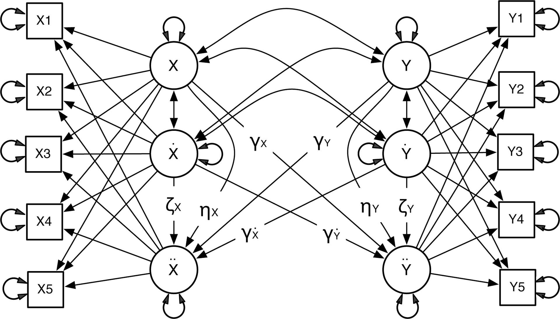
Coupled Latent Differential Equation Model (Coupled LDE).

Related Technical Issues

The Issue of Centering

Whether to center data before analysis is an important consideration. According to Equation 1, x is the displacement of a variable from its equilibrium. So the effect on the second derivative is the deviation from the equilibrium rather than a raw score. Thus, we recommend conducting within-person centering around their equilibrium. If the equilibrium is known, the equilibrium value should be subtracted from each score. If the equilibrium is unknown, one reasonable alternative is to use an individual’s mean as an estimate of his or her equilibrium. By this procedure, the equilibrium or the estimated equilibrium is removed from analysis and leaves only fluctuations. Not centering data could result in serious bias in estimation, especially when there are large individual differences in equilibrium. The following simulation shows how centering improves estimation when there are individual differences in equilibrium.

Simulation.

We simulated a 200-occasion single oscillator with a frequency parameter η = −0.05 and damping parameter ζ = 0, separately for two persons. The difference between the equilibria of the two persons (Δequilibrium) was varied from 0.2 to 3.0 times the total variance. The simulation was repeated 100 times. The data were either centered or left uncentered before fitting a single LDE model (Figure 2). The mean and standard deviation of the 100 trials are presented in Table 1.

Table 1.

Distance between two person’s equilibria and estimated frequency parameter using uncentered and centered data.

	η Simulated	η estimated with uncentered data	η estimated with centered data
Δequilibrium = 0.2SD	η = −0.05	−0.055(0.0011)	−0.056(0.0010)
Δequilibrium = 0.4SD	η = −0.05	−0.053(0.0013)	−0.056(0.0012)
Δequilibrium = 0.6SD	η = −0.05	−0.049(0.0015)	−0.056(0.0011)
Δequilibrium = 0.8SD	η = −0.05	−0.045(0.0012)	−0.056(0.0011)
Δequilibrium = 1.0SD	η = −0.05	−0.040(−0.0013)	−0.056(0.0012)
Δequilibrium = 1.2SD	η = −0.05	−0.035(0.0012)	−0.056(0.0012)
Δequilibrium = 1.4SD	η = −0.05	−0.031(0.0013)	−0.056(0.0012)
Δequilibrium = 2.0SD	η = −0.05	−0.021(0.0009)	−0.056(0.0009)
Δequilibrium = 3.0SD	η = −0.05	−0.012(0.0004)	−0.056(0.0011)

Result.

As shown in Table 1, when Δequilibrium is small, for example within 1.0 SD of the total variance, the estimated parameter based on uncentered data (−0.055, −0.053, −0.049, −0.045, −0.040) is close to the true value −0.05. However, as Δequilibrium increases, the bias in estimation grows. In contrast, the estimation based on within-person centered data is not influenced by individual differences in equilibria, because these differences have already been removed by within-person centering. Within-person centering avoids bias induced by individual differences in equilibrium. There are other sources of bias, such as the amount of noise in data. So the estimated η is not exactly the same as the simulated value. A careful selection of smoothing parameter D can reduce bias induced by noise, which will be elaborated next.

The Issue of Smoothing

As mentioned before, the smoothing parameter D is critical in creating time-delay embedded data. Previously, the fit indices of LDE model, such as the Akaike information criterion (AIC) and the −2 log-likelihood (−2LL) have been recommended as criteria to set the parameter D (Boker & Nesselroade, 2002). Here we recommend a new criterion: if we plot the estimated frequency parameter η as a function of D, the optimal value for D occurs just after the estimated frequency parameter η becomes stable. The following simulation shows the details of this criterion and the advantage of using the estimated parameter value as a criterion compared with using fit indices.

Simulation.

A second order linear differential equation (as in Equation 1) with ζ = 0 and η set to −0.01, −0.05 or −0.01 was simulated with 200 observations. To investigate influences of noise in data, the signal-to-noise ratio (SNR) was set to 2:1, 1:1 or 1:2. SNR is a measure that compares the level of a signal of interest to the level of background noise. Here SNR is specified as the ratio of the variance of the simulated data to the variance of the normally distributed numbers added to the data. Then time-delay embedding matrices were constructed as in Equation 3, letting D vary from 3 to 30. A single LDE model was fitted separately for each time delay embedded matrix. Then the true and estimated η, model AIC, and −2LL were plotted against the embedding dimension D. Figure 4 shows the time series plot of the simulated data and how the estimated value of η, AIC and −2LL changed with the embedding dimension D. Figures 4(a), (b) and (c) plot η = −0.005 for all three SNR conditions, and (c) and (d) plot η = −0.01 with SNR = 1 : 1, and η = −0.001 with SNR = 1 : 1.

Figure 4.

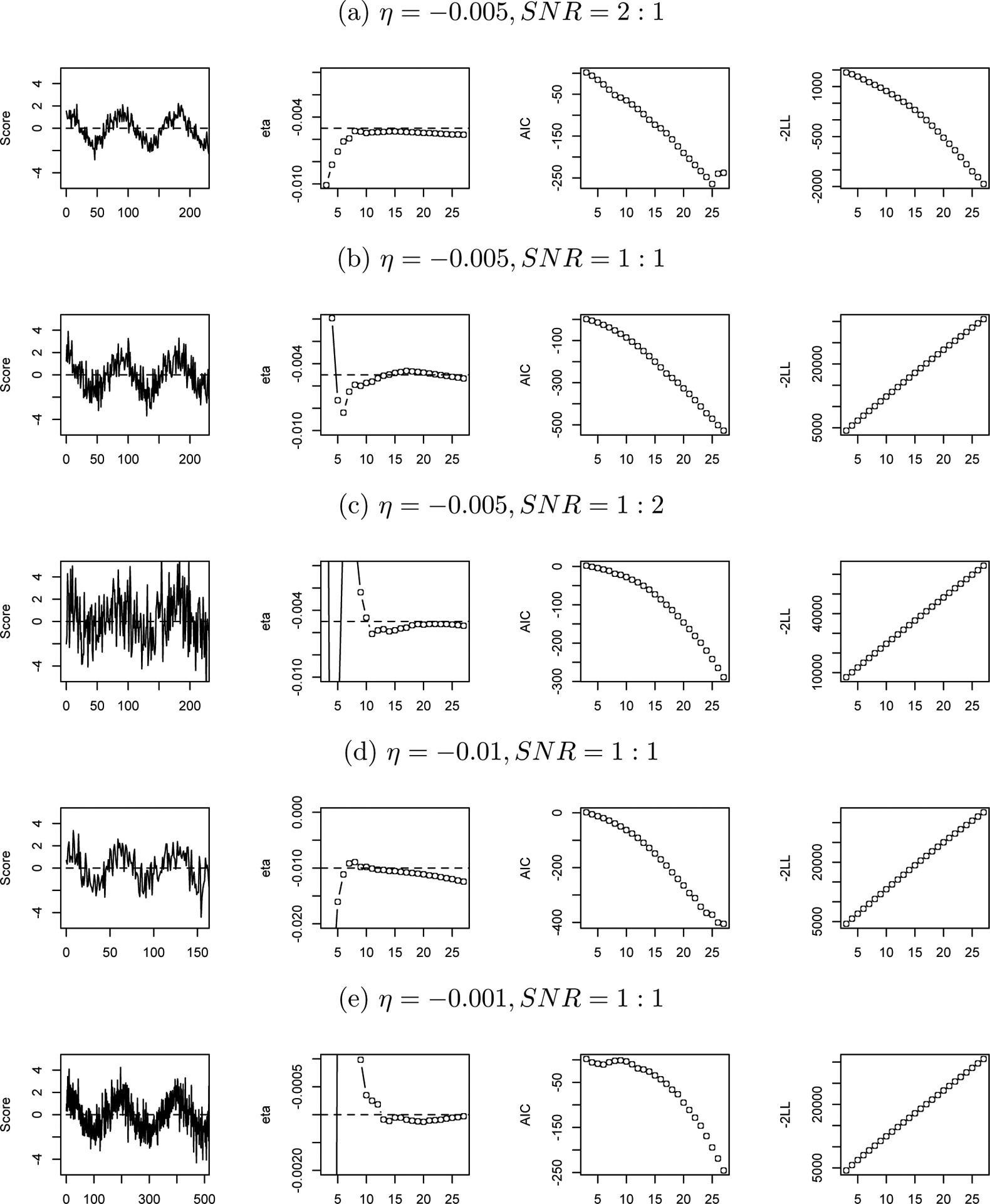
Relationship between D and Estimated η, AIC and −2LL.

Note: In each condition (a, b, c, d, e), from left to right, the first plot presents the simulated time series, in which the horizontal axis stands for time and the horizontal dash line indicates the equilibrium; the second plot presents how the estimated η change with the time delay embedding dimension D, in which the horizontal dash line indicates the true value of η; the third plot presents model AIC against D; and the last plot presents −2LL against D.

Results.

As shown in the second column of Figure 4, under all simulation conditions, the accurate estimate of η occurs just after the estimated η becomes stable. For example, for condition (a), the optimal value of D is around 8, and for condition (e), this value is around 13. However, in the plots of D against AIC and −2LL (see the third and the fourth columns of Figure 4), there is nothing special about these optimal values. Most of the time, AIC and −2LL are linear functions of D. The result that the model fit index (AIC and −2LL) is not a good criterion is not surprising, because theoretically it is a measure of the relative goodness of fit of a statistical model given a set of data. However, by altering dimensions of time delay embedding, what we actually do here is alter the number of rows of data used to fit a given model. So AIC and −2LL are not suitable criteria in this case. We recommend to use the estimated η as the criteria instead of the model fit index to select the value of D.

This simulation also shows how SNR and the value of η influences the choice of D. If we decrease the SNR, i.e., increase the noise, then only a narrow range of D values could produce reasonable estimates of η. For example, from condition (a) to (c), the SNR decreases from 2:1 to 1:2, and the choice of D shrinks from a range with 8 as its lower bound to a range with 18 as its lower bound. This result implies that when there is more noise in the data, one must be more careful in choosing D, since the proper values of D are limited. As the true η becomes closer to zero, i.e., the frequency becomes slower, the value of D that produces the best estimate of η increases. For example, in condition (d), η = −0.01 and the optimal D is around 6, in condition (b), η = −0.005 and the optimal D is around 12, and in condition (e), η = −0.001 and the optimal D is around 15. This result suggests that if a high frequency of fluctuations is expected, it is better to use a smaller D.

Simulation work supported our idea that the optimal D occurs when the estimated η becomes stable. Note that D values within the stable range are all acceptable. We suggested the starting value of the stable range because it is the smallest D to obtain an accurate estimation. A smaller D means a shorter time segment to calculate derivatives, which will give us more data to use. Also note that the width of the stable range varies under different conditions: sometimes wider, sometimes narrower, depending on the frequency of the oscillation and the amount of noise. In extreme cases, for example, very short oscillations, the “stable” state holds only at a single value of D, then the estimation goes into a precipitous decline. In those cases, “the inflection point” is a better term than “the start of the stable range”.

Knowing how to center and smooth data is enough for the need of implementing single LDE models. However, when the system becomes more complicated, we need to know more. The next two sections will deal with coupled systems and systems with moderators.

Coupled Systems

A coupled system is a system with two variables interacting with each other or where one influences the other. Figure 3 shows a bi-directional coupled LDE model, which includes two self-regulating systems and some coupling effect between them. The meaning of the frequency parameter η and the damping parameter ζ in the self-regulating systems have been explained before. However, the interpretation of the coupling parameters may be unclear to many readers. We now clarify the meaning of the coupling parameters by simulation.

To investigate how one variable influences the other variable in a coupled system, two variables x and y were simulated according to Equation 4, where γ_x and γ_ẋ represent a unidirectional coupling effect of x and ẋ on ÿ.

$$\begin{gathered} \ddot{x}={\eta }_{x}x+{\zeta }_x\dot{x}+{ϵ}_x \\ \ddot{y}={\eta }_{y}y+{\zeta }_y\dot{y}+{\gamma }_{x}x+{\gamma }_{\dot{x}}\dot{x}+{ϵ}_y \end{gathered}$$ (4)

To illustrate the effects of unidirectional coupling, γ_x and γ_ẋ were by turns set to zero and the results are plotted in Figure 5. Figure 5a shows that γ_x = 0 and γ_ẋ > 0 indicates a phase synchronizing effect of x on y (0° offset), while γ_x = 0 and γ_ẋ < 0 indicates a phase desynchronizing effect (180° offset). The absolute value of γ_ẋ determines how fast y will be synchronized or desynchronized by x. A large absolute value indicates a strong effect of x on y and will result in a quickly synchronizing and desynchronizing system. And a small absolute value will take a long time before y will be synchronized or desynchronized by x. Figure 5b shows that γ_ẋ = 0 and γ_x > 0 indicates y is dragged back by x (270° offset), while γ_ẋ = 0 and γ_x < 0 indicates y is pushed forward by x (90° offset). Again, the absolute value of γ_x determines how rapidly the system reaches a steady state.

Figure 5.

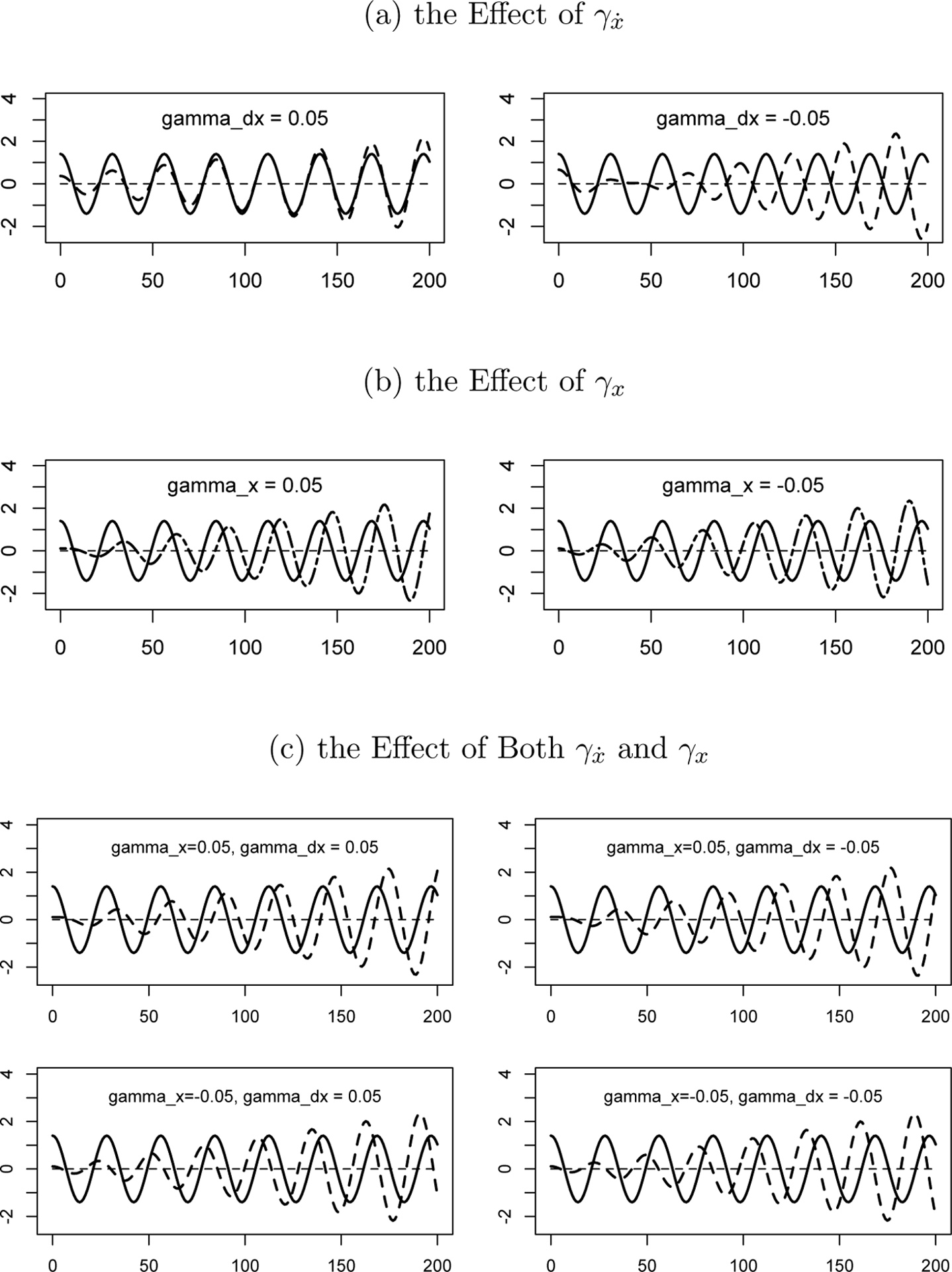
Demonstration of γ Parameters.

Note: The horizontal axis stands for time, the vertical axis stands for score, the solid line denotes x and the dashed line denotes y.

Next both γ_x and γ_ẋ were set to be nonzero in order to understand their synergistic effect. As Figure 5c shows, the combination results in some offset between x and y. The exact degree of offset depends on the sign and the relative size of γ_x and γ_ẋ. It is hard to tell the differences between these conditions by eye. The next question is whether the coupled LDE models are able to estimate the coupling parameters accurately. Again, we will use simulation to answer this question.

Two 200-occasion coupled processes were simulated (x and y), where η_x = −0.05, and η_y was set to be one of the values: −0.01, −0.02, −0.03, −0.04, −0.05, −0.06, −0.07, −0.08, and −0.09. To test the coupling effect of x on ÿ, γ_x was set to a value from an equal interval sequence of length 100 with min = −0.05 and max = 0.05, and γ_ẋ was set to zero. To test the coupling effect of ẋ on ÿ, γ_ẋ was selected from an equal interval sequence of length 100 with min = −0.2 and max = 0.2, and γ_x was set to zero. Table 2 is a summary of all 1800 simulated conditions. The rationale for choice of the range of γ_x and γ_ẋ will be explained in detail in the discussion part of this section.

Table 2.

Simulation conditions based on Equation 5.

			test γx		test γẋ
η Conditon	ηx	ηy	γx	γẋ	γx	γẋ
1	−0.05	−0.01	(−0.05 – 0.05)	0	0	(−0.2 – 0.2)
2	−0.05	−0.02	(−0.05 – 0.05)	0	0	(−0.2 – 0.2)
3	−0.05	−0.03	(−0.05 – 0.05)	0	0	(−0.2 – 0.2)
4	−0.05	−0.04	(−0.05 – 0.05)	0	0	(−0.2 – 0.2)
5	−0.05	−0.05	(−0.05 – 0.05)	0	0	(−0.2 – 0.2)
6	−0.05	−0.06	(−0.05 – 0.05)	0	0	(−0.2 – 0.2)
7	−0.05	−0.07	(−0.05 – 0.05)	0	0	(−0.2 – 0.2)
8	−0.05	−0.08	(−0.05 – 0.05)	0	0	(−0.2 – 0.2)
9	−0.05	−0.09	(−0.05 – 0.05)	0	0	(−0.2 – 0.2)

Note: (−0.05 – 0.05) stands for a value from an equal interval sequence of length 100 with min = −0.05 and max = 0.05; and (−0.2 – 0.2) stands for a value from an equal interval sequence of length 100 with min = −0.2 and max = 0.2

Next, a coupled LDE model was fit to the simulated data. The true values of the coupling parameters from the simulation are plotted against the estimated values of the coupling parameters from the LDE model in Figure 6 and 7. The closer these points are to the 45° slope line, the closer the estimated values are to the true values.

Figure 6.

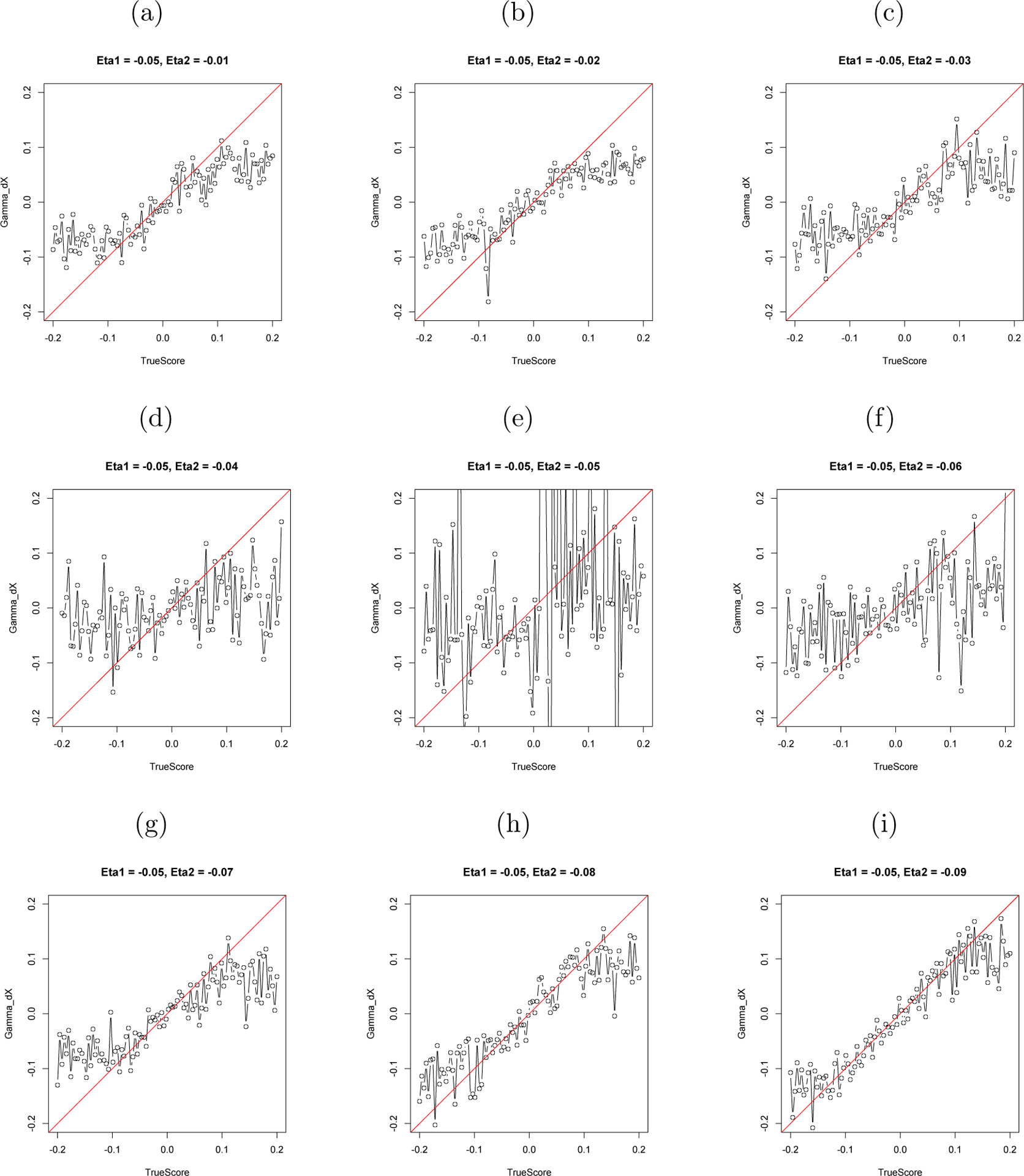
The Estimated γ_ẋ and the True Value of γ_ẋ.

Note: The horizontal axis stands for the simulated value of γ_ẋ and the vertical axis stands for the estimated value of γ_ẋ.

Figure 7.

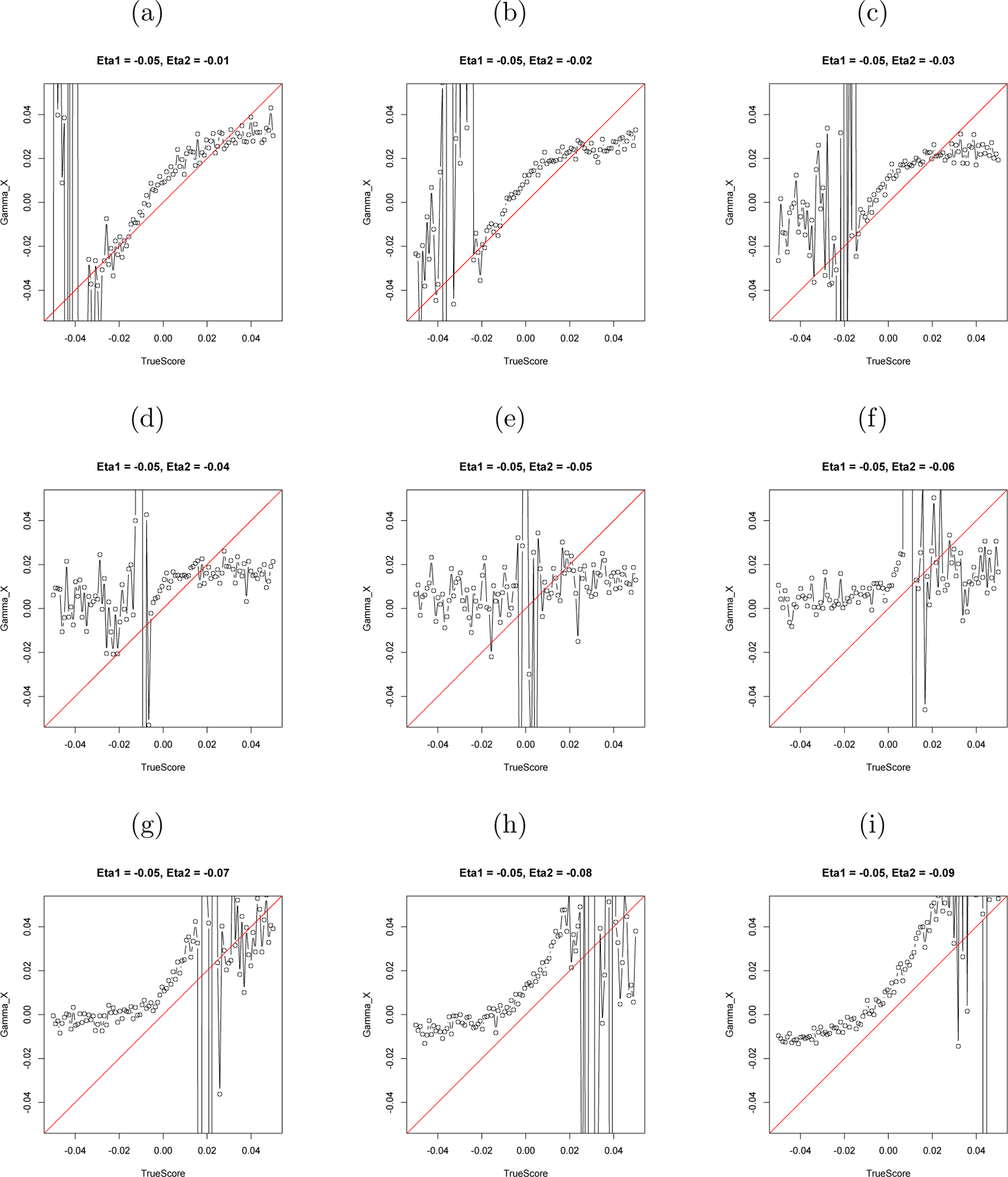
The Estimated γ_x and the True Value of γ_x.

Note: The horizontal axis stands for the simulated value of γ_x and the vertical axis stands for the estimated value of γ_x.

As Figures 6 and 7 show, the accuracy of the estimation of γ_ẋ and γ_x depends in part on the closeness of η_x and η_y. When η_x = η_y, the estimation breaks down. Upon reflection, the result that the coupling parameters cannot be estimated when the two variables have the same self-regulating frequency is not surprising. If the two variables have the same intrinsic frequency, it is impossible to determine whether there is an interaction between them or if it is the result of two same frequency self-regulations. Consider the motion of your legs while walking. If we only have the legs’ movement data, we cannot tell whether each leg has its own drive, whether they drive each other, or whether there is an external synchronizing driver. The equal frequency problem here is just like the collinearity problem in regression. We cannot put two completely correlated variables into one regression. However, human behavior is so complicated that behavioral variables are rarely perfectly phase locked and synchronized together with same frequency. So researchers in social science may encounter the equal frequency problem only rarely.

Next, notice that accurate estimation of both γ_ẋ and γ_x happens only in a certain range of γ values in our simulation. For γ_ẋ, this range is −0.1 ~ 0.1, which would vary depending on η and the difference between two ηs. Exceeding this range, the estimation becomes inaccurate. And for γ_x, the range is −0.02 ~ 0.02. Even within this range, the estimate of γ_x is systematically larger than the true value; the majority of the points are above the 45° line. Also note that the range reported here may be specific to the particular simulated condition (η ≈ −0.05). In other frequency conditions, the range of accurately estimated γ might differ from that reported here. This simulation implies that some boundary restrictions on the relative value of coupling parameters γ in compared with the value of η are needed in order to obtain accurate estimations. However, considering the size of η, the range of γ is quite wide, indicating that the estimation fails only when the coupling effect (x → ÿ) is much larger than the regulating effect (y → ÿ). In that case, researchers may want to reconsider the relationship between two variables. Maybe they are not two coupled processes, but one is directly driving the other. In that case, they should be considered as one process. For example, measures of husband’s happiness and measures of wife’s happiness might be two coupled processes, and measures of husband’s happiness and measures of his self-esteem might be a single process with two entities.

Adding Moderators

Moderator variables are widely used in psychological research when studying multiple heterogeneous groups or multiple occasions of measurement. In dynamical system analysis, moderators are of particular importance since individuals could express individual differences in multiple ways: frequency and amplitude of intrinsic regulation, and pattern of coupling.

Equation 5 shows the logic of moderator analysis, in which x stands for a predictor variable, y an indicator variable, and z a moderator variable. The subscript i refers to person i, and j refers to occasion of measurement j. In Equation 5, b_0i is set to be zero because we have centered all variables, and the intercept (i.e. equilibrium value) is thus fixed to zero. The residual part ∈_1ix_ij + e_ij is represented by ∈_ij .

$$\begin{gathered} y_{ij}=b_{0i}+b_{1i}{x}_{ij}+e_{ij} \\ {b}_{0i}={\mu }_0+c_0{z}_i+{ϵ}_{0i} \\ {b}_{1i}={\mu }_1+c_1{z}_i+{ϵ}_{1i} \\ {y}_{ij}=\underset{0}{\underbrace{{\mu }_0+c_0{z}_i+{ϵ}_{0i}}}+{\mu }_1{x}_{ij}+c_1{z}_i{x}_{ij}+\underset{{ϵ}_{ij}}{\underbrace{{ϵ}_{1i}{x}_{ij}+e_{ij}}} \\ =\left({\mu }_1+c_1{z}_i\right)x_{ij}+{ϵ}_{ij} \end{gathered}$$ (5)

By substituting Equation 1, in which ẍ is the indicator, x and ẋ are the predictors, into Equation 5, a differential equation with moderator z can be formed (Equation 6). Note that the moderator z is not a repeated-measure variable, so it only has subscript i but not j. So for a person i with moderator z_i, her individual frequency parameter should be η₀ + η₁z_i, and her damping parameter should be ζ₀ + ζ₁z_i. Since each person has a z_i score, their oscillation will have an individualized frequency and damping.

$${\ddot{x}}_{ij}=\left({\eta }_0+{\eta }_1{z}_i\right)x_{ij}+\left({\zeta }_0+{\zeta }_1{z}_i\right){\dot{x}}_{ij}+{ϵ}_{ij}$$ (6)

Figure 8 illustrates how Equation 6 is implemented in a single LDE model. D1 and D2 are placeholders, with zero mean and zero variance. The coefficient of the direct pathway from x to ẍ (η₀) is estimated, the first coefficient of the indirect pathway is fixed to be the value of the moderator (z_i), and the second coefficient η₁ is to be estimated. Thus the indirect pathway represents the moderating effect z_i × η₁. Some SEM programs, e.g., OpenMx (Boker et al., 2011), can specify the coefficient of a pathway to be values that are specific to each row in the data matrix. The same setting is made for the direct and indirect pathways from ẋ to ẍ. Significant η₁ or ζ₁ indicates a significant moderating effect.

Figure 8.

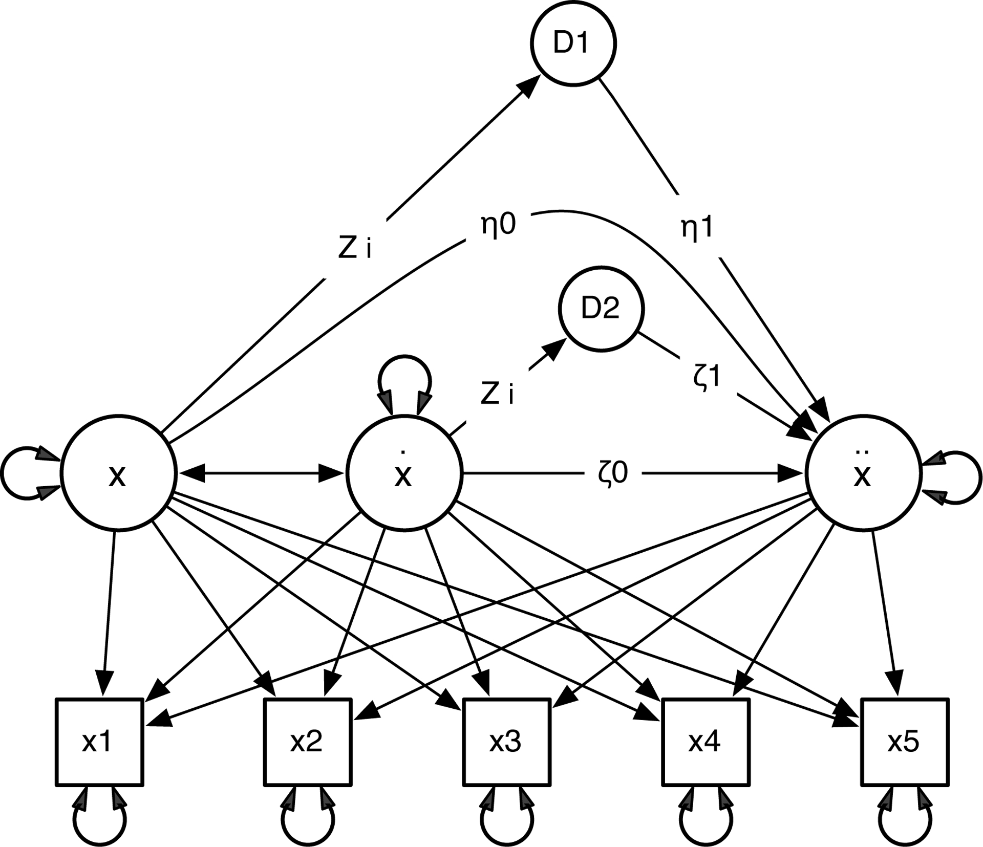
Single LDE Model with Moderator.

Data Source

LDE and Coupled LDE models are applicable to a variety of psychological phenomena and human dynamic systems. The example analysis will model the dynamics between the changes in ovarian hormones and the fluctuations in eating in a sample of young women to illustrate how an LDE model can be implemented with empirical data. Previous studies (Edler, Lipson, & Keel, 2007; Klump, Culbert, Edler, & Keel, 2008; Klump et al., 2012) have used primarily regression-based methods to show that changes in estradiol 3 are associated with changes in eating behavior across the menstrual cycle. These associations appear to be independent of daily changes in negative affect (Edler et al., 2007; Klump et al., 2008), although no study to date has investigated the dynamic coupling between these variables, or examined the extent to which negative affect moderates (rather than mediates) these associations. An LDE coupled model analysis with moderators would shed light on these issues by estimating relationships between estradiol, eating, and negative affect and determining the nature and direction of associations between the variables.

The example data comes from an on-going study at Michigan State University (Klump et al., 2012) that includes 198 female twins who provided 45-days of behavioral ratings and salivary hormone samples. Variables of interest for the current analysis include daily salivary estradiol levels and ratings of emotional eating (a measure of the tendency to eat in the presence of negative emotions, using the Emotional Eating subscale of the Dutch Eating Behavior Questionnaire, Van Strien, Frijters, Bergers, & Defares, 1986) and negative affect (Negative Affectivity subscale of Positive and Negative Affect Schedule, Watson, Clark, & Tellegen, 1988).

Step-by-Step Analysis and Results

Step 1: Centering data.

One hundred and ninety-eight participants completed the experiment. Of these, 181 participants had ovulatory menstrual cycles. Since ovulation is a key period of hormonal change during the menstrual cycle, and women who do not ovulate evidence minimal changes in estradiol levels, the data of those who did not ovulate were excluded from analysis. Table 3 presents the mean and the standard deviation of the variables of interest. Within-person centering was conducted to remove individual differences in equilibrium.

Table 3.

Descriptive statistics of variables of interest (n=181, measures=45)

	Estradiol level (pg/ml)	Eating	Negative Affect
N	6328	7639	7634
Missing	1817	506	511
Mean	3.18	1.35	15.31
S.D.	2.12	0.49	5.56

Step 2: Time delay embedding.

The parameters D in time-delay embedding can affect estimation of derivatives. To find an optimal embedded dimension D, we tried a range of values (5 ≤ D ≤ 15) and fit the single oscillator LDE model to the eating data for each value of D. We use the range 5 – 15 based on experience. Readers can try from 3 to the total number of measures in your own data. Figure 9 shows that the value of estimated η starts to become stable around 9. So the time-delay embedding dimension D was set to 9. Note that Figure 9 is very similar to the simulation plot Figure 4a, which supports the utility of the simulation results for applications to real data.

Figure 9.

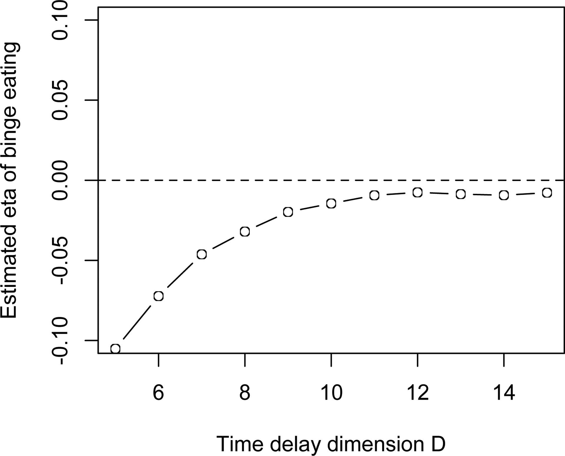
Time-delay Embedded D and Estimated η of Emotional Eating.

Step 3: Fit a single LDE model.

If we use D = 9 to embed the data, we obtain parameter estimates η = −0.026 (p < .01), and ζ = −0.059 (p < .01). The significant negative η suggests that if a woman emotionally eats more than normal, there will be a self-regulation process driving her to eat less and back to the equilibrium; similarly when she emotionally eats less than normal, there will be also a force pushing her to eat more. The significant negative ζ suggests that a sudden increase in emotional eating will produce a stronger tendency to reduce emotional eating than a slow increase; similarly a sudden decrease will produce a stronger tendency to increase than a slow decrease. Substituting η and ζ into Equation 2 gives an estimated period of emotional eating oscillation of approximately 40 days. The same procedure was conducted for estradiol. The estimated η = −0.039 (p < .01), and the estimated ζ = −0.027 (p > .05). The period of estradiol change is approximately 27 days.

Step 4: Fit a coupled LDE model.

Two separate coupled LDE models were fit to test whether estradiol and negative affect have coupling effects on emotional eating. Results are presented in Table 4, in which the EAT-EST Model estimates the relationship between emotional eating and estradiol levels, and the EAT-NA Model estimates the relationship between emotional eating and negative affect. None of the coupling effects between eating and negative affect is significant, indicating that eating and negative affect are not coupled with each other. In comparison, the coupling effect between estradiol levels and eating is significant, γ_Ėst = .049 (p < .05), and γ_Ėat = −.062 (p < .05), indicating that estradiol levels and emotional eating are coupled with each other. Next, all γ parameters in the EAT-EST Model were set to zero to specify an uncoupled model. As shown in Table 5, compared with the completely coupled model, the uncoupled model fit worse, with higher AIC and Δχ²/Δdf = (17.2 + 0.6)/4 = 4.45 > 3.8. So the coupling effect between estradiol levels and eating was supported by AIC and also by the likelihood ratio difference test. There is no difference between the χ² of the Coupled Models 1 and 2, Δχ²/Δdf = 0.6/2 = 0.3 < 3.8. So considering parsimony (AIC), Coupled Model 2 is the best model, in which estradiol level and eating are only coupled by their first derivatives. The results of model comparison are consistent with the significance test.

Table 4.

Parameters estimation of coupled differential equation model.

EAT-EST Model			EAT-NA Model
Parameter	Estimation	S.E.	Parameter	Estimation	S.E.
ηEat	−.025	.004	ηEat	−.018	.006
ζEat	−.069	.021	ζEat	−.074	.004
ηEst	−.037	.004	ηNA	−.058	.008
ζEst	−.026	.016	ζNA	−.050	.023
γEst	.002	.003	γNA	−.014	.008
γĖst	.049	.016	γṄA	.022	.041
γEat	−.002	.004	γEat	.010	.006
γĖat	−.062	.022	γĖat	.011	.023

Table 5.

Fit indices for uncoupled model and coupled models.

	Coupling parameters	χ2	df	Δ − 2LL	Δdf	AIC	RMSEA
Coupled Model 1	γEst, γĖst, γEat, γĖat	2569.8	149	0	0	2271.8	0.049
Coupled Model 2	γĖst, γĖat	2570.4	151	0.6	2	2268.4	0.049
Uncoupled Model	-	2587.6	153	17.2	2	2281.6	0.049

The coupled LDE model suggests that estradiol and emotional eating are coupled with each other. Since they are coupled by their first derivatives, as suggested by simulations, estradiol synchronizes eating, and eating desynchronizes estradiol, so the two regulation process are not completely phase locked. To illustrate the coupling effect between estradiol and emotional eating, we simulated two coupled time series using parameters in Table 4, and plot them on the left panel of Figure 10. On the right panel, we present the population aggregated mean of standardized estradiol level and emotional eating score in each phase of menstrual cycle (ovulatory, mid-luteal, premenstrual and follicular). As shown in the figure, emotional eating reaches its peak after estradiol reaches its peak. In the menstrual cycle, this is the time after ovulation but before the next menstruation. This result is consistent with previous findings (Klump et al., 2012) that emotional eating scores were highest during the mid-luteal phase which occurs after ovulation but before next menstruation.

Figure 10.

Simulated and Aggregated Time Series of Emotional Eating and Estradiol.

Step 5: Fit a moderated LDE.

The coupled LDE model suggested that negative affect has no coupling effect on emotional eating. It is possible, however, that negative affect influences eating indirectly as a moderator of the intrinsic regulation of eating or as a moderator of estradiol’s effect on eating. We consequently tested the moderator effect of the mean negative affect score (meanNA), which is an estimate of the average level of negative emotion across the 45 days of the study, in the Eating single LDE model, and in the Eating-Estradiol coupled LDE model.

As shown in Table 6, the average level of negative affect has a significant moderating effect in the single LDE model, η_{Eat_1} = −.016 (p < .05). The significant negative η_{Eat_1} implies that higher average levels of negative affect are associated with faster frequency of emotional eating oscillation. Figure 11 plots the emotional eating regulation of two typical participants. The participant with meanNA=−1.15 has a lower frequency of oscillation, and the participant with meanNA=1.13 has a higher frequency of oscillation.

Table 6.

Moderating effect of average negative affect.

Model	Parameter	Estimation	S.E.
EAT Single LDE with moderator meanNA	ηEat_0	−.016	.004
	ηEat_1	−.011	.003
	ζEat	−.046	.024
EAT-EST Coupled LDE with moderator meanNA	ηEst	−.035	.004
	ζEst	−.012	.022
	ηEat	−.008	.004
	ζEat	−.070	.023
	γĖst_0	.427	.042
	γĖst_1	.590	.045
	γĖat_0	−.046	.025
	γĖat_1	−.010	.018

Figure 11.

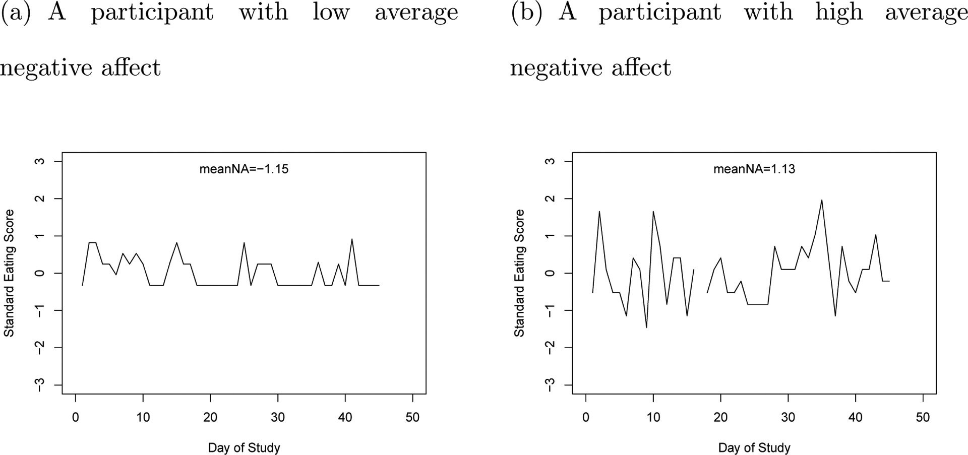
The Emotional Eating Regulation of Two Example Participants.

The moderating effect of meanNA on the coupling between two processes was also tested. The procedure was similar to testing the moderation of η, but instead influenced the coupling parameters γ_Ėst and γ_Ėat in Figure 3. Results from this moderated coupled LDE model suggest that meanNA has a significant moderating effect on the coupling between estradiol and eating, as show in Table 6, γ_{Ėst_1} = .590 (p < .01), the same direction with γ_{Ėst_0}. This implies that a high NA person’s emotional eating behavior is more strongly coupled with hormone estradiol, whereas a low NA person’s emotional eating behavior is less affected by estradiol.

Can we trust this Differential equation model?

With the help of an LDE model, we found some interesting relations between variable derivatives. Yet there exist some potential doubts: are these results an artifact of the method that we employed to calculate the derivatives rather than a property of the data? Can we trust that these findings are not just numerical coincidence? To address these questions, we employed permutation tests (Fisher, 1935; Welch, 1990), frequently called surrogate data tests (Theiler, Eubank, Longtin, & Galdrikian, 1992) in the dynamical systems literature, using two ways of shuffling data.

Within-person Shuffling was used to remove the time dependent information in the time series. We randomly rearranged the order of observations for each person. This removes the time dependent information in the time series (Schreiber & Schmitz, 2000). In this way, we guarantee that a null hypothesis of no internal dynamic process is true, and therefore a significant η should only be detected at approximately the rate specified by the chosen α level. Data were shuffled in this way 1000 times and a single LDE model was fitted to the shuffled data. Thus, we obtained 1000 estimates of the η parameter when the null hypothesis was true. Among these 1000 models, 890 did not converge, 67 converged but had a positive η which indicates no oscillation and self-regulation. Thus, the probability of obtaining a negative estimate of η is 1 − (895 + 67)/1000 = 3.8% < 5%. In summary, in the un-shuffled data, the LDE model detected a significant negative η; and when the dynamics were destroyed, the model did not detect it. Within-person shuffling supported the use of LDE models to estimate self-regulation.

Between-person Shuffling was used to remove the interaction between two dynamic processes. We used one randomly selected person’s hormone levels to predict another randomly selected person’s emotional eating scores (we made sure they were not twins), without changing the order of observations within person. In this way, we guaranteed that the null hypothesis of no coupling between estradiol levels and emotional eating was true, while the self-regulation of each process was retained. Thus after shuffling, the coupled LDE model should estimate η and ζ the same as before, while γs should be distributed around a mean of zero, implying no coupling effect. Data was shuffled in this way 1000 times and a coupled LDE model was fitted to the shuffled data. Thus, we obtained 1000 estimates for each parameter in the coupled LDE model. Figure 12 plots the distribution of these 1000 parameter estimates from the shuffled data, the dashed vertical line marks its 95% confidence interval around zero, and the solid vertical line marks the parameter estimate from the original un-shuffled data. As expected, all η and ζ stayed the same after shuffling, while the γs had a peak at zero with a confidence interval excluding the significant effect we found from the original data. Between-person shuffling supported the use of coupled LDE to estimate coupling effects between two regulating behaviors.

Figure 12.

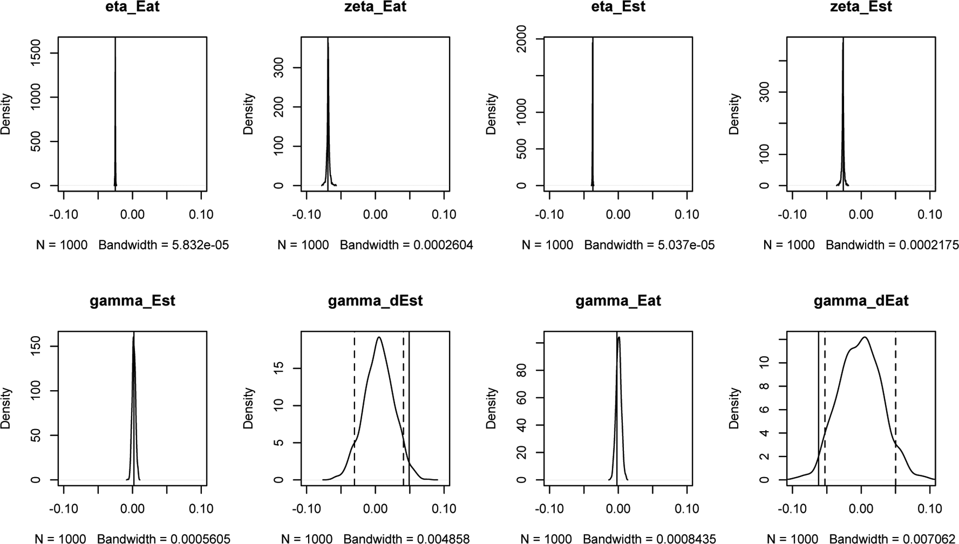
Shu e Data Between Person and Fit a Coupled LDE.

Note: the density plot shows the distribution of 1000 estimated parameters based on the shuffled data, the dashed vertical line marks its 95% confidence interval, and the solid vertical line indicates the estimated parameters base on the original data.

Data shuffling enhanced our confidence in LDE models: they were unlikely to find dynamics in time series that did not have dynamics and they were unlikely to find coupling between two unrelated variables.

Discussion

The present study used simulations and a set of real data to explore several issues related to differential equation models. We recommended an innovative way to find the proper time-delay embedding dimension D, investigated the conditions for accurate coupling parameter estimation, explored the use of a moderated LDE model in real data, and created a between-person shuffling method to test the coupled LDE models under the null-hypothesis.

This article demonstrated a procedure for implementing basic LDE models. Readers might have some concerns about the real situations, such as “what if there is no oscillation”,“what if phase and amplitude frequently reset”, and so on. In fact, LDE models can handle these concerns. They specify the relationship between derivatives, and thus shed light on a system’s change in velocity given its current location and velocity. Implementing an LDE model does not require a full period of oscillation or even any oscillation at all. For example, the study on the well-being of recently bereaved widows (Bisconti et al., 2004) does not include a periodical oscillation, since this kind of situation cannot happen again and again. Also phase and amplitude resetting does not matter, since the relationship between derivatives would not change because of resetting (Deboeck, Boker, & Bergeman, 2008). This is an advantage of differential equation modeling over other trajectory estimation methods.

Another concern readers might have is the sufficient number of measures for implementing this method. To calculate a second order derivative requires a minimum of three observations (Deboeck, Montpetit, Bergeman, & Boker, 2009). However, it has been proved that using only three occasions of measurement to estimate the derivatives might have biased estimates of the dynamical parameters, and measurement error can be mistaken as high frequency signal (Boker & Nesselroade, 2002). So usually more than three occasions of measurement are recommended, with the interval between occasions less than 1/8 of the length of a single period of oscillation (Boker et al., 2003). With a large number of measures, each participant would have several rows of data, which allows a random effect of individual in parameter estimation. In other words, each participant could have his or her own dynamical parameters. However, if each participant only has few occasions of measurement, we must aggregate people together to estimate an average value of each parameter.

Besides these basic concerns, some readers might want to explore advanced topics. For example, the equilibrium might not be constant. In that case, researchers can first construct a model for equilibrium change. The type of model will depend on their theory for the system’s equilibrium. Then an LDE model can be used to model the residuals from the equilibrium model (Boker & Bisconti, 2006). Another expansion of LDE models is LDE models with random effects. Individuals might have distinct dynamics, such as personalized frequency parameters and damping parameters. Advanced users can specify the parameters of LDE models with random effects of individual differences. Another concern is that the linear differential equation introduced here might not be sufficient to describe nonstationarities in the data. For example, the η and ζ parameters may change along with time. The issue of nonstationarity is beyond the scope of this article. People who are interested can read some articles mainly focused on non-linear and nonstationary dynamical systems (e.g., Busemeyer & Townsend, 1993; Boker & Graham, 1998; Boker, Xu, Rotondo, & King, 2002; Butner et al., 2005; Chow, Ferrer, & Nesselroade, 2007; Finan et al., 2010).

Limitations and Future Directions

The example data only include 45 days of observations. The total interval of observation is shorter than two complete cycles, which is often regarded as a strengthening condition for the period analysis. For the menstrual cycle, we know it is around 28 days, which is close to our estimation. For emotional eating behavior, we have no independent confirmation that it follows a periodic cycle of 40 days. However, what we can conclude is that emotional eating behavior is a self-regulating system. People adjust their future behavior based on their current state.

Another limitation is related with the coupled LDE models. As we discussed in the issue of coupling, the coupled LDE model still needs to be explored, especially with respect to restrictions on parameter setting, such as boundaries for γ parameters, and the difference between two ηs. This study explored several conditions and found the approximate boundaries under those conditions. More general conclusions and an algebraic proof of this requirement are needed.

References

- Amazeen PG, Amazeen EL, & Turvey MT (1998). Timing of behavior: Neural, computational, and psychological perspectives In Rosenbaum DA & Collyer CE (Eds.), Dynamics of human intersegmental coordination: Theory and research. Cambridge, MA: MIT Press. [Google Scholar]
- Beek PJ, Schmidt RC, Morris AW, Sim M-Y, & Turvey MT (1995). Linear and nonlinear sti ness and friction in biological rhythmic movements. Biological Cybernetics, 73 , 499–507. [DOI] [PubMed] [Google Scholar]
- Beltrami EJ (1987). Mathematics for dynamic modeling. NY: Academic Press. [Google Scholar]
- Bisconti TL, Bergeman CS, & Boker SM (2004). Emotional well-being in recently bereaved widows: a dynamical systems approach. Journal of Gerontology: Psychological Sciences, 59 (4), 158–167. [DOI] [PubMed] [Google Scholar]
- Boker SM, & Bisconti TL (2006). Dynamical systems modeling in aging research In Bergeman CS & Boker SM (Eds.), Methodological issues in aging research (p. 185–229). Mahwah, NJ: Lawrence Erlbaum Associates, Inc. [Google Scholar]
- Boker SM, & Graham J (1998). A dynamical systems analysis of adolescent substance abuse. Multivariate Behavioral Research, 33 (4), 497–507. [DOI] [PubMed] [Google Scholar]
- Boker SM, Neal M, Maes H, Wilde M, Spiegel M, Brick T, et al. (2011). Openmx: An open source extended structural equation modeling framework. Psychometrika, 76 (2), 306–317. [DOI] [PMC free article] [PubMed] [Google Scholar]
- Boker SM, Neale MC, & Rausch JR (2003). Latent differential equation modeling with multivariate multi-occasion indicators In van Montfort HOK & Satorra A (Eds.), Recent developments on structural equation models: Theory and applications (p. 151–174). Amsterdam: Kluwer. [Google Scholar]
- Boker SM, & Nesselroade JR (2002). A method for modeling the intrinsic dynamics of intraindividual variability: Recovering the parameters of simulated oscillators in multi-wave panel data. Multivariate Behavioral Research, 37 (1), 127–160. [DOI] [PubMed] [Google Scholar]
- Boker SM, Xu M, Rotondo JL, & King K (2002). Windowed cross–correlation and peak picking for the analysis of variability in the association between behavioral time series. Psychological Methods, 7 (1), 338–355. [DOI] [PubMed] [Google Scholar]
- Box GEP, Jenkins GM, & Reinsel GC (1970). Time series analysis: Forecasting and control (4th ed.). A John Wiley and Sons, Inc., Publication. [Google Scholar]
- Busemeyer JR, & Townsend JT (1993). Decision field theory: A dynamic cognition approach to decision making. Psychological Review, 100 , 432–459. [DOI] [PubMed] [Google Scholar]
- Butner J, Amazeen PG, & Mulvey GM (2005). Multilevel modeling of two cyclical processes: extending differential structural equation modeling to nonlinear coupled systems. Psychological Methods, 10 (2), 159–177. [DOI] [PubMed] [Google Scholar]
- Chow S-M, Ferrer E, & Nesselroade JR (2007). An unscented kalman filter approach to the estimation of nonlinear dynamical systems models. Multivariate Behavioral Research, 42 , 283–321. [DOI] [PubMed] [Google Scholar]
- Chow S-M, Ram N, Boker SM, Fujita F, & Clore G (2005). Emotion as a thermostat: representing emotion regulation using a damped oscillator model. Emotion, 5 (2), 208–225. [DOI] [PubMed] [Google Scholar]
- Deboeck PR, Boker SM, & Bergeman C (2008). Modeling individual damped linear oscillator processes with differential equations: Using surrogate data analysis to estimate the smoothing parameter. Multivariate Behavioral Research, 43 (4), 497–523. [DOI] [PMC free article] [PubMed] [Google Scholar]
- Deboeck PR, Montpetit MA, Bergeman CS, & Boker SM (2009). Describing intraindividual variability at multiple time scales using derivative estimates. Psychological Methods, 14 (4), 267–386. [DOI] [PMC free article] [PubMed] [Google Scholar]
- Duncan TE, Duncan SC, Strycker AL, Li F, & Alpert A (1999). An introduction to latent variable growth curve modeling: Concepts, issues, and applications. New Jersey, Mahwah: Lawrence Erlbaum Associates, Inc. [Google Scholar]
- Edler C, Lipson SF, & Keel PK (2007). Ovarian hormones and binge eating in bulimia nervosa. (Vol. 37) (No. 1). Department of Psychology, University of Iowa, IA 52242, USA.. [DOI] [PubMed] [Google Scholar]
- Finan PH, P. H., Hessler EE, Amazeen PG, Butner J, Zautra AJ, & Tennen H (2010). Oscillations in daily pain prediction accuracy. Nonlinear Dynamics, Psychology, and Life Sciences, 14 (1), 27–46. [PMC free article] [PubMed] [Google Scholar]
- Fisher RA (1935). The design of experiment. New York: Hafner. [Google Scholar]
- Hajek O (1968). Dynamical systems in the plane. Boston, MA: Academic Press. [Google Scholar]
- Klump K, Culbert KM, Edler C, & Keel PK (2008). Ovarian hormones and binge eating: Exploring associations in community samples. Psychological Medicine, 38 (12), 1749–1757. [DOI] [PMC free article] [PubMed] [Google Scholar]
- Klump K, Keel PK, Racine S, Burt SA, Neal M, Sisk CL, et al. (2012, August 13). The interactive effects of estrogen and progesterone on changes in binge eating across the menstrual cycle. Journal of Abnormal Psychology. Available from Advance online publication. doi: 10.1037/a0029524 [DOI] [PMC free article] [PubMed] [Google Scholar]
- McCall RB, & Appelbaum MI (1973). Bias in the analysis of repeated-measures designs:some alternative approaches. Child Development, 44 (3), 401–415. [Google Scholar]
- Montpetit MA, Bergeman CS, Deboeck PR, Tiberio SS, & Boker SM (2010). Resilience-as-process: negative affect, stress, and coupled dynamical systems. Psychology and Aging, 25 (3), 631–640. [DOI] [PubMed] [Google Scholar]
- Noakes L (1991). The takens embedding theorem. International Journal of Bifurcation and Chaos, 4 (1), 867–872. [Google Scholar]
- Odgers L, Candice, Mulvey EP, Skeem JL, Gardner W, Lidz CW, & Schubert C (2009). Capturing the ebb and flow of psychiatric symptoms with dynamical systems models. The American Journal of Psychiatry, 166 (5), 575–582. [DOI] [PubMed] [Google Scholar]
- Ong AD, Bergeman CS, & Boker SM (2009, December). Resilience comes of age: defining features in later adulthood. Journal of Personality, 77 (6), 1777–1804. [DOI] [PMC free article] [PubMed] [Google Scholar]
- Raudenbush SW, & Bryk AS (2002). Hierarchical linear models: applications and data analysis methods (2nd ed ed., Vol. 1). Thousand Oaks: Sage Publications. [Google Scholar]
- Schreiber T, & Schmitz A (2000). Surrogate time series. Physica D: Nonlinear Phenomena, 142 , 346–382. [Google Scholar]
- Theiler J, Eubank S, Longtin A, & Galdrikian B (1992). Testing for nonlinearity in time series: the method of surrogate data. Physica D: Nonlinear Phenomena, 58 , 77–94. [Google Scholar]
- Van Strien T, Frijters JER, Bergers GPA, & Defares PB (1986). Dutch eating behaviour questionnaire for assessment of restrained, emotional and external eating behaviour. International Journal of Eating Disorders, 5 , 295–315. [Google Scholar]
- Von Oertzen T, & Boker SM (2010). Time delay embedding increases estimation precision of models of intraindividual variability. Psychometrika, 75 (1), 158–175. [DOI] [PMC free article] [PubMed] [Google Scholar]
- Watson D, Clark LA, & Tellegen A (1988). Development of validation of brief measures of positive and negative affects: The panas scales. Journal of Personality and Social Psychology, 47 , 1063–1070. [DOI] [PubMed] [Google Scholar]
- Welch WJ (1990). Construction of permutation tests. Journal of American Statistical Association, 85 , 693–698. [Google Scholar]