In Vivo Confocal Imaging of Fluorescently Labelled Microbubbles: Implications for Ultrasound Localization Microscopy

Abstract

We report the time kinetics of fluorescently labelled microbubbles in capillary-level microvasculature as measured via confocal microscopy and compare these results to ultrasound localization microscopy. The observed 19.4 ± 4.2 microbubbles per confocal field-of-view (212 μm x 212 μm) is in excellent agreement with the expected count of 19.1 microbubbles per frame. The estimated time to fully perfuse this capillary network was 193 seconds, which corroborates the values reported in literature. We then modeled the capillary network as an empirically determined discrete-time Markov chain with adjustable microbubble transition probabilities though individual capillaries. Monte Carlo random walk simulations found perfusion times ranging from 24.5 seconds for unbiased Markov chains up to 182 seconds for heterogeneous flow distributions. This pilot study confirms a probability-derived explanation for the long acquisition times required for super-resolution ultrasound localization microscopy.

I. Introduction

ULTRASOUND localization microscopy (ULM) is a super-resolution imaging technique that overcomes the conventional diffraction limit of ultrasound imaging by exploiting the unique acoustic properties of contrast microbubbles (MBs) in vasculature [1]–[5]. ULM processing results in an approximately tenfold improvement in vascular imaging resolution [1] while preserving clinically relevant penetration depths and maintaining the safety, low-cost, and lack of ionizing radiation of ultrasound. Thus, ULM offers unprecedented clinical significance by providing noninvasive, in vivo blood flow information potentially down to the capillary scale—which may be critical in informing a broad spectrum of pathological disease states. However, ULM is currently limited by long imaging acquisition times for full reconstruction of microvascular networks, which represents a substantial barrier to clinical translation of the technique. A prevailing hypothesis is that these long acquisition times are a natural consequence of the rare occurrence of MB passage in capillary vessels [6], [7]. Conversely, previous studies have demonstrated that MB signal becomes attenuated inside capillaries due to constraints in volumetric expansion from vessel walls [8]–[11], which may partially explain the difficulty in reconstructing capillary networks with ULM.

A number of different investigators have explored the fundamental trade-off between ULM microvascular fidelity and imaging acquisition times. Dencks et al. [12] investigated the minimum time required to reconstruct microvascular trees via ULM from murine tumor xenografts. They reported 90% microvessel mapping times, based on an exponential saturation fitting, of 50 to 101 seconds. Hingot et al. [6] compared the relationship between ULM pixel reconstruction size and acquisition time in the murine brain, finding a characteristic time of 76.8 seconds for ULM reconstructions at 5 μm. This corresponds to a 90% saturation time of 230.4 seconds. Christensen-Jeffries et al. [7] developed a Poisson statistical model to predict ULM acquisition times for generalized imaging conditions and target vasculature. When applying their model to the experimental conditions reported in Dencks et al.’s work they found estimated perfusion times ranging from 78 to 139 seconds. The salient conclusion from these studies is that the long acquisition times required for ULM reconstruction of microvasculature is inherently a consequence of vessel physiology, flow rates, and the low probability of MB passage through capillaries. It is worth noting, however, that the standards that are often used in investigations of ULM performance are either ultrasound imaging itself (i.e.: comparing long acquisition times to shorter duration subsets) or are histological metrics that provide static physiological quantifications (e.g.: microvascular density) which may be difficult to register to a corresponding imaging plane.

The objective of this article is to explore flow kinetics of MBs in vivo using high framerate ultrasound and confocal microscopy as MBs traverse through the chorioallantoic membrane (CAM) of chicken embryos. The ex ovo CAM offers an excellent exploratory model for MB flow kinetics due to the well-organized planar vascular bed developed by the membrane, which is optically transparent and readily accessible. This permits rapid co-registered acoustic-optic studies of MB transit using multiple imaging modalities. Confocal microscopy provides an imaging resolution that is in the sub-micron range and thus serves as a reliable benchmark for identification of fluorescently-labelled MBs. Here, we report that the time kinetics of fluorescently-labelled MBs, taken from the superficial vascular bed of the CAM, are in good agreement with a probability-derived explanation for long acquisition times required for ULM imaging. Confocal imaging allowed for the visualization of MBs as they traversed through the CAM vessel bed. It was noted that there was a heterogeneous distribution of MBs through this capillary bed, leading to some capillary segments being rarely traversed by MBs. We then modeled this capillary bed as an empirically determined discrete-time Markov chain network and estimated perfusion times using a Monte Carlo random-walk simulation. The effect of adjusting the node-to-node transition weightings on the network coverage time was also explored. This Monte Carlo simulation permitted the investigation of rare MB passage events on the anticipated 90% saturation time for a physiologically relevant network connection topology. We found that unbalanced transition probabilities, arising from heterogeneous MB flow through the capillary bed, can extend the estimate for full perfusion by at least an order of magnitude.

The rest of this paper is structured as follows: in Section II, we introduce the ex ovo CAM preparation, the steps involved in super-resolution ULM imaging, and the confocal imaging procedure, along with the Monte-Carlo simulation details. In Section III, we show the results of estimates for time to complete perfusion based on ULM imaging, confocal imaging, and Monte-Carlo simulations. We then discuss these results in Section IV, and provide a conclusion.

II. Materials and Methods

A. Ex ovo CAM preparation

Avian embryos, such as the CAM model used in this study, are not considered to be “live vertebrate animals” under NIH PHS policy. As such, no IACUC approval was necessary to conduct the research presented in this paper.

Fertilized chicken eggs (white leghorn) were obtained from Hoover’s Hatchery (Rudd, IA) and immediately placed into an incubator upon receipt (Digital Sportsman Cabinet Incubator 1502, GQF). This was counted as the first day of embryonic development (EDD-01). On EDD-04 the egg shells were removed with the aid of a rotary dremel tool, and the egg contents were transferred into plastic weigh boats prepared with acoustic windows. Embryos were kept in a humidified incubator (Caron model 7003-33) until imaging on EDD-18. A total of three chicken embryos were used in this pilot study.

A vial of ‘target-ready’ Vevo Micromarker (FUJIFILM VisualSonics) was reconstituted with 1 mL PBS and 0.25 μg Biotin-4-fluorscein, yielding a solution of 2 × 10⁹ FITC-labelled MBs/mL. A solution of rhodamine lectin (lens culinaris agglutinin) was prepared in advance of imaging at a 1 to 10 dilution with PBS. Prior to injection, glass capillary needles were produced by pulling borosilicate glass tubes (1.20mm x 0.69mm x 10cm, Sutter Instruments, Novato, CA, USA) with a PC-100 glass puller (Narishige, Setagaya City, Japan) and fitted onto Tygon^® R-3603 laboratory tubing. On EDD-18 the surface vasculature of the CAM was cannulated with the glass capillary needle and 100 μL of the rhodamine lectin solution was injected to fluorescently label the vascular endothelium [13]. Following this, the embryo was returned to the incubator for 15 minutes to allow for complete recirculation and labelling of the lectin. Immediately prior to imaging, the CAM membrane was injected with a 70 μL bolus of FITC-labelled MBs.

B. Ultrasound imaging

Ultrasound images were acquired using a Vantage 256 system (Verasonics Inc., Kirkland, WA). A high-frequency linear array transducer (L35-16vX, Verasonics Inc.) was placed on the side of the plastic weigh boat housing the CAM to image through the acoustic window. Center frequency was 20 MHz, selected to reconstruct a capillary-scale super-resolved image [14]. Imaging was performed using a 9-angle plane wave compounding sequence (1° increment step) with a post-compounding frame rate of 1,000 Hz for a total acquisition length of 32 s (32,000 frames). Ultrasound images were stored as in-phase quadrature (IQ) datasets of 1,600 frames each for analysis in MATLAB.

Super resolution MB localization and velocity maps were reconstructed at a 5 μm axial/lateral resolution following the methodology presented in [5]. Briefly, each IQ dataset was reshaped into a 2D Casorati matrix and separated into singular values via SVD decomposition. A low order threshold was applied to filter out tissue background [15], where the threshold was determined by the decay rate of the singular value curve [5] – a threshold value of 10 for each 1,600 frame dataset. A filtered Casorati matrix was generated via inverse SVD and reshaped back into the original cineloop dimensions. A normalized cross-correlation was then performed on each frame of the cineloop with a Gaussian function, representing the point-spread function of an individual MB, to localize MB centroids. MBs trajectories were then reconstructed using a normalized cross-correlation algorithm to track MB movement and velocity [4].

Optical microscopy was performed simultaneously with ULM imaging using a Nikon SMZ18 stereomicroscope (Nikon, Tokyo, Japan) at 4x magnification to confirm reconstruction of vascular features. A diagrammatic example of the optical-acoustic imaging set-up is shown in Fig. 1, demonstrating multiscale optical validation coinciding with acoustic imaging. Following acoustic imaging, a region of interest was selected on the CAM membrane and confocal microscopy was performed to generate capillary-level vacular images and to optically track individual FITC-MBs.

Fig. 1.

A) Diagrammatic example of the co-registered optical-acoustic imaging set-up used in this experiment. B) Chicken embryos were positioned under the stereomicroscope with the ultrasound transducer was coupled to the side of weigh-boat. C) SVD filtered ultrasound image of CAM vasculature, demonstrating microbubble events. D) Optical image that served as a reference standard for ULM imaging. E) Confocal imaging of the CAM vasculature demonstrates a honey-comb-like capillary bed.

The optical and acoustic datasets were then spatially co-registered to confirm the accurate reconstruction of vasculature via ULM processing, as is shown in Fig. 2.

Fig. 2.

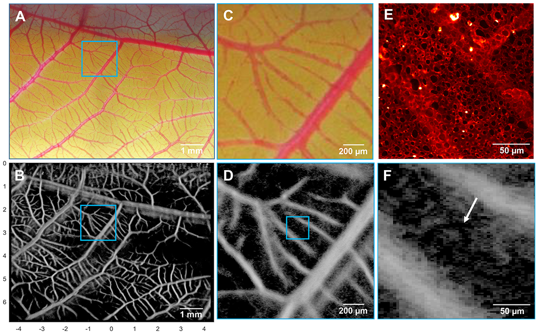
A) Optical microscopy image was co-registered with the ultrasound imaging plane, and allowed for the identification, localization, and verification of vessels detected by ULM. B) ULM image of the corresponding CAM vessel network, yielding a similar vascular structure. C) A higher magnification optical image was acquired to investigate the performance of D) ULM at the arteriole/venule scale. E) Confocal imaging of the superficial capillary layer demonstrates a characteristic hexagonal microvascular bed, which was partially recovered with F) ULM imaging (arrow). Note: the confocal image shown in (E) is for demonstrative purposes only, and was not taken from the same CAM membrane shown in the other image panels.

C. Confocal imaging

Laser-scanning confocal images were acquired using a Nikon A1R+ system following intravascular injection of FITC-labelled Vevo Micromarker MBs and CAM endothelial vessels labelled with rhodamine lectin. Multispectral data was acquired using eGFP (emission wavelength 525 nm) and tdTomato (emission wavelength 595 nm) channels. Confocal images had a 212 μm x 212 μm field-of-view (FOV), 0.414 μm isotropic resolution, and framerate of 14.7 Hz. Images were digitized at 16 bits using an integrated digital camera and saved as .nd2 format. Fig. 3 demonstrates a representative example image of a confocal imaging FOV used in this study.

Fig. 3.

A) Confocal imaging of the superficial CAM vascular bed. The vascular lumen is stained with rhodamine lectin (red channel), and MBs were labelled with FITC (green channel). Black spaces are stromal space. B) A further magnified image of the vessel bed highlights the polydisperse size distribution MBs. C) An example of a large MB event, indicating potential MB aggregation.

Image channels were split and then exported as .PNG files for offline analysis in MATLAB. MBs were detected using a 2D normalized cross-correlation on the eGFP channel data with a hypothetical 2D Gaussian bubble profile [16]. A cross-correlation threshold of 0.5 was used to reject low confidence MB detections and total MB counts were generated for each frame by enumerating isolated MB regions (Fig. 5). MB diameters were then estimated from the eGFP channel data, assuming a circular cross-section (Fig. 4). This was validated using an AccuSizer single-particle optical sizing system (Model 780, Particle Sizing Systems, Santa Barbara, CA, USA) on a 10 μL sample of the FITC-MB conjugate. The blood volume of each confocal field of view was estimated using watershed segmentation with manually selected seed points placed on stromal regions within the FOV. The number of capillary segments within each confocal plane was estimated using Voronoi tessellation (e.g., “voronoi.m” in Matlab) on centroids of CAM stromal spaces. An example of this processing is demonstrated in Fig. 6.

Fig. 5.

The number of MBs detected per confocal frame. A) and B) were from a shorter pilot imaging set from the same CAM. C) and D) were from the second embryo, and E) from the final embryo in this study. The average of the five imaging acquisitions yielded an average of 19.4 ± 4.2 MBs per confocal FOV.

Fig. 4.

A) Empirical density function of MB diameters, with median diameter indicated with a dotted line, which was confirmed with B) an AccuSizer 780 particle sizer.

Fig. 6.

A) The isolated rhodamine channel data was used to estimate the vascular volume and number of capillary ‘segments’ within the confocal FOV. B) A corresponding Voronoi tessellation of the centroids (red dots) of the CAM stromal space (white segmentation). The detected paths (blue lines) were used as an estimate for the number and length of capillaries in the CAM model. C) Temporal MB centroid projection (green) on CAM microvasculature (red). D) Diagrammatic example of network edge weighting adjustments, where transition probabilities were altered to account for connection lengths and detect MB centroids.

D. Wash-in function

Next, we estimated the total time it would take to completely perfuse the capillary bed with MBs (i.e.: the time taken to reconstruct the entire vascular network under ideal conditions). We first accumulated all of the ULM datasets to produce saturation curves, as demonstrated in Fig. 7. We then generated empirical wash-in curves for the confocal data using a temporal maximum intensity projection of the MB centroid positions (Fig. 8). The following mono-exponential wash-in function was fit to all datasets:

$$C\left(t\right)=C_0(1-e^{-\kappa t})$$ (1)

where C₀ is the saturation level of the curve (assumed to be 100% of the vascular lumen), t is time in seconds, and κ is a rate constant. The above model was taken as equivalent to the exponential saturation model used in Dencks et al. [12].

Fig. 7.

A) Reference optical image of a ULM region of interest. B) ULM accumulation saturation curve, yielding a characteristic time of 7.1 second (21.4 second saturation time). C) Example ULM images taken at different time steps (1.6, 6.4, and 22.4 seconds) to demonstrate gradual saturation of the reconstruction.

Fig. 8.

CAM microvasculature (red) with temporal MB centroid projections (gray). The arrows highlight regions with few MB passage events, indicating rarely perfused capillaries. (Right column) The cumulative area of the confocal FOV filled with MBs during the acquisition, with fitted curve.

E. Discrete-time Markov chain Monte Carlo simulations

As an alternative technique to estimate the time to full perfusion, we represented the CAM vessel bed as an empirically determined undirected discrete-time Markov chain network. This permitted us to examine the effect of adjusting the network transition weights on the overall perfusion time for a physiologically relevant topology. The network adjacency matrix was constructed via Voronoi tessellation (“voronoi.m” in Matlab) of CAM stromal space centroids (Fig. 6), where network nodes were defined as the end-point intersections of Voronoi line segments. Monte Carlo random walks on this empirically determined network were initialized by randomly selecting a starting node position from a uniform distribution for the “walker’s” location, representing a single MB in the capillary bed. Each subsequent step of the MB walker was performed by randomly selecting a neighboring network node with the transition probability weighted by the network adjacency matrix. This was done to estimate the cover time of the network nodes (vertices) and the network edges (connections), where edge cover time is indicative of MB traversal in all capillary segments and thus the 90% saturation time.

It is worth noting that a discrete-time Markov chain network with unweighted transition probabilities represents the lower bound for cover times. In order to get a more realistic estimate for the time to traverse the Markov chain network we adjusted the relative weighting, or traversal probabilities, for each network edge. Briefly, for each node position, we adjusted the normalized edge transition probabilities to be proportionate to the relative connection lengths, such that longer vessels had proportionally lower transition probabilities. This was referred to as the distance-weighted network. We also produced network weightings where the edge transition probabilities were proportional to the number, or density, of detected MB centroids from the confocal images. This centroid-weighted network had a substantial bias to a select few ‘high flow’ vascular pathways, capturing the flow heterogeneity observed in the confocal video. A diagrammatic example of this weighting procedure is depicted in Fig. 6. Finally we combined the two weighted adjacency matrices together via a normalized Hadamard product to account for both features simultaneously.

III. Results

A. Ultrasound Localization Microscopy

ULM imaging of the CAM vessel bed was able to accurately localize microvascular flow within arterioles and venules with diameters on the order of tens of microns, as confirmed by optical imaging (Fig. 2). The characteristic hexagonal shape of the CAM microvasculature was partially recovered by ULM imaging, however we failed to reconstruct all of the vascular features on the scale of capillaries (<10 μm). When reviewing the SVD filtered IQ cineloops we were able to observe MB signals within inflowing and outflowing vasculature, but much of the MB signal disappeared during traversal of the capillary bed (Video 1). The planar nature of the CAM is such that there must be a direct capillary connection between arterioles and venules, implying that there must be a change in the MB backscatter during capillary passage.

B. Microbubble flow kinetics

Confocal imaging demonstrated a polydisperse size distribution of FITC-labelled MBs, as illustrated in Fig. 3 and Fig. 4. The median diameter of MBs was found to be 2.5 μm, which is within the range reported by the manufacturer (2.3 – 2.9 μm) (VisualSonics PN11691). The largest observed MB diameter was 6.7 μm, potentially indicating MB aggregation. The eGFP channel cross-correlation technique outlined in Section II–C yielded an average of 19.4 ± 4.2 MBs per confocal FOV, as depicted in Fig. 5. An example of MB tracking on confocal data can be seen in Video 2. In order to validate this observation, we first estimated the blood volume of the CAM membrane using the rhodamine channel data. Manual segmentations of the vascular space found that approximately 76% of the confocal FOV was comprised of vascular lumen and yielded an estimate for blood volume of 3.4 x 10⁵ μm³, or 3.4 x 10⁻⁴ μL of blood, assuming that the membrane thickness is 10 μm. This relatively high area percentage of vascular lumen was expected as the CAM is analogous to lung tissue for the developing embryo, and therefore requires a high blood to surface area ratio for efficient gas exchange.

Given that the injection volume of MBs was 70 μL and that the reported concentration of Vevo Micromarker is 2 × 10⁹ MB/mL, we can assume that the total number of injected MBs is on the order of 1.4 × 10⁸ MBs per bolus. Chicken embryos at this stage of development (EDD-18) have an approximate total blood volume of 2.5 mL [17]. Thus, we estimate that the MB concentration in chicken blood was 5.6 × 10⁷ MBs per mL of blood. Multiplying this result with the estimate of blood volume in the confocal FOV yields an estimate of 19.1 MBs per confocal imaging frame. This result, in combination with the finding that some of the detected MBs diameters were less than 1 μm, could be taken as evidence that some MB rupture may have occurred following the bolus injection into CAM vasculature (i.e. the smallest detected MBs may be phospholipid shell fragments). One can also note the bimodal nature of the MB size distribution, with a subpopulation of large diameter MBs. We speculate that these represent MB aggregates (Fig. 3).

C. Estimated time to fully perfuse capillary bed

The fitting for the confocal data yielded an average rate constant κ = 2.21 × 10⁻⁴ s⁻¹, which corresponds to an estimated 708 seconds required to reach a 90% vascular perfusion. Applying this rate constant directly overestimates the time for total perfusion, as our confocal imaging acquisition was temporally sparse (14.7 Hz) relative to the typical flow speeds found in capillaries (~1 mm/s). The ideal minimum frame rate would be one in which no new pixels occupied by moving MBs are missed during the idle time between two consecutive confocal frames. We posit that this frame rate would correspond to a MB moving by half its diameter per time step, and thus by temporally interpolating our maximum intensity projection by this factor we will be able to recover the missing microbubble signals that would have been captured with such frame rate. Using the median of MB diameters found in this study (2.5 μm) and an assumed MB velocity of 1 mm/s, this corresponds to a minimum time step of 1.25 ms, or a frame rate of 800 Hz. This then yields an estimated time to 90% perfusion of 13 seconds based on the rate constant derived from Eq. (1).

Hingot et al. [6] found a characteristic time of 76.8 seconds for ULM reconstructions at a pixel size of 5 μm, corresponding to a saturation time of 230.4 seconds (defined as 90% perfusion). However, their experiment involved the injection of 400 μL of Sonovue (average concentration of 3 x 10⁸ MBs/mL [18]) into a 500 gram rat. The circulating blood volume in rats is estimated to be 64 mL/kg [19], leading to MB concentration of 3.75 x 10⁶ MBs per mL of blood in their experiment. This is roughly 14.9 times lower than our MB concentration of 5.6 x 10⁷ MBs per mL of blood, as detailed above. Linearly scaling our estimates by this difference in MB concentration yields a time to 90% perfusion of 193 seconds, and corresponding characteristic time of 64.3 seconds. Likewise, the report by Dencks et al. [12] used a 50 μL bolus of MBs at a concentration of 2 x 10⁸ MBs/mL. The estimated blood volume for a 25 gram mouse is around 1.8 mL [19], yielding a MB blood concentration of 5.56 x 10⁶ MBs per mL of blood. Scaling our estimates by this ratio of MB concentration results in a 90% perfusion time of 131 seconds.

The saturation curves generated from the ULM dataset (Fig. 7) generated an average rate constant of κ = 0.14 s⁻¹. This corresponds to a characteristic time of 7.1 seconds and a 90% perfusion time of 21.4 seconds. Scaling these results by the difference in MB concentration yields a characteristic time of 106 seconds, with a saturation time of 319 seconds. It is worth noting that the high concentration of MBs used in this study necessitated discarding several overlapping MB events, potential extending the saturation time.

D. Monte Carlo simulation perfusion times

A Voronoi tessellation of the CAM vessel bed, as demonstrated in Fig. 6, yielded a total of 225 vertices (branching points) and 345 connections (or capillary segments) with a median length of 14.1 μm. The results of 1000 Monte Carlo simulations on this network are demonstrated in Fig. 9.

Fig. 9.

Cover times for 1000 Monte Carlo simulations of a discrete time Markov chain network generated using Voronoi tessellation of the CAM vessel bed. A) The coverage of network nodes, and B) the coverage for the network edges. The solid line is the mean result, and the band is the standard deviation of the simulations.

The average 90% edge cover time of this discrete-time Markov chain network was found to be 31.7 seconds (2,260 walker steps), under the assumption of a MB velocity of 1 mm/s and a measured median edge length of 14.1 μm. Given that the cover time for k independent walkers (i.e. MBs in the network) is linearly proportional to the cover time of a single walk [20], we can scale this result by number of MBs detected per frame. Thus, we estimate that it would take just 1.64 seconds for 19.4 MBs to traverse this network. Adjusting this result to the difference in MB concentration from the paper by Hingot et al. [6] yields a total perfusion time of 24.5 seconds.

As mentioned previously, a discrete-time Markov chain network with unweighted transition probabilities will have the fastest cover times of this topology. Thus, we used the edge path lengths and detected MB centroids (Fig. 6) to adjust the relative weighting (or traversal probabilities) for each network edge, as described in Section II–E. Adjusting the weighting of the adjacency matrices had a net effect of increasing the network coverage times (Table I).

TABLE I:

Estimated Saturation Times

Method	Microbubble Concentration (MBs per mL blood)	Time to 90% MB perfusion (seconds)	MB perfusion time adjusted to common blood concentration (seconds)
Dencks et al. [12]	5.56 x 106	101	150
Christensen-Jeffries et al. [7]	5.56 x 106	139	206
Hingot et al. [6]	3.75 x 106	230.4	230.4
ULM CAM saturation	5.6 x 107	21.4	319
Confocal wash-in	5.6 x 107	13	193
Markov-chain (unweighted)	5.6 x 107	1.6	24.5
Markov-chain (distance-weighted)	5.6 x 107	3.5	51.8
Markov-chain (centroid-weighted)	5.6 x 107	5.9	88.3
Markov-chain (distance- and centroid-weighted)	5.6 x 107	12.2	182

The average edge cover time of the distance-weighted network was 4,790 steps, which corresponds to a traversal time of 51.8 seconds under the assumptions outlined for the unweighted Markov-chain network above. The 90% coverage time for the centroid-weighted network was 8,150 steps, yielding a saturation time of 88.3 seconds. Finally, the combined weighted network had the longest coverage time at 16,800 steps. This corresponds to a saturation time of 182 seconds, which is on the same order of magnitude as the values reported by Hingot et al. [6], Dencks et al. [12], and Christensen-Jeffries et al. [7]. These results are summarized in Table 1, along with their corresponding MB concentrations. Table 1 reports the direct estimates of MB 90% perfusion time, in addition to the 90% perfusion times adjusted to a common blood concentration (the MB concentration reported by Hingot et al. [6]).

IV. Discussion

In this pilot study, we reported the time kinetics of fluorescently labelled MBs in capillary-level microvasculature as measured via confocal microscopy. We observed 19.4 ± 4.2 MBs per confocal field of view (212 μm x 212 μm), which is in excellent agreement to the expected blood flow-rate count of 19.1 MBs per frame. The estimated time for MBs to traverse this capillary network was 193 seconds based on wash-in curves generated from the confocal data, and 182 seconds for a discrete-time Markov chain Monte Carlo simulation where the network transition probabilities were weighted by vessel length and MB centroid density. Saturation curves of our ULM dataset yielded a time estimate of 319 seconds. These results are consistent with the characteristic time for 5 μm ULM reconstruction reported by Hingot et al.[6], and on the same order of magnitude as the 90% exponential saturation time reported by Dencks et al. [12], and the generalized MB perfusion model developed by Christensen-Jeffries et al. [7].

While ULM imaging of the CAM was able to accurately localize microvascular flow down to the tens of microns scale (i.e., arterioles and venules), we had difficulty fully reconstructing capillary level MB flow in the CAM (Fig. 2). This is surprising given the high density of MBs found within the relatively small FOV of confocal imaging. Interestingly, we were able to observe MBs on Bmode images and with ULM from both inflowing and outflowing vasculature, but the MB signal became silent during traversal of the capillary bed. One possible explanation is that low capillary compliance is prohibiting the volumetric oscillations of MBs [8]–[11], resulting in reduced signal backscatter. The effect of confinement leading to a reduction in MB oscillation has been previously reported in chicken embryos [21], and this may be compounded by the relatively low hydrostatic pressure in CAM capillary vessels.

Laser-scanning confocal imaging was used as the gold-standard in this study to confirm the blood-flow kinetics of MBs as they traversed the CAM capillary bed. However, the framerate achieved in our experimental design for a 212 μm x 212 μm FOV was slow (14.7 Hz) relative to the expected speed of MBs (~1 mm/s). This low framerate is an inherent limitation of the two wavelength resonant confocal imaging used in this study. As a consequence, the fluorescent imaging presented in this study may have missed some of the MB passage events. We attempted to correct for this by scaling our temporally sparse acquisition by a hypothetical ideal minimum frame rate to recover more realistic estimates of total perfusion times. Although this approach produced perfusion estimates that are consistent with literature (193 seconds vs. 230.4 seconds [6]), it is not an ideal solution given that it cannot account for completely missed MB events. Furthermore, the low framerate may have influenced the weightings applied to centroid-weighted Markov-chain simulation, as MB passage through particularly fast vessels may have been missed. Confocal imaging is also limited in its ability to accurately measure MB diameters as the narrow imaging slab thickness might intersect MB at various heights. This, in turn, may explain the wide distribution of MB diameters seen in Fig. 4.

Another limitation of this study is the high concentration of MBs used in both ULM and optical imaging. This invariably leads to a substantial amount of MB signal overlap for ULM reconstruction, increasing the localization uncertainty, and necessitating a longer acquisition time. This may, in part, explain the relatively high estimate for ULM 90% saturation time found in this study (319 seconds). Furthermore, the assumption that all saturation times can be linearly scaled by the difference in MB concentration requires that passage of individual MBs are independent from one another, and is potentially an oversimplification of more complication MB flow kinetics and interactions (e.g.: aggregation). Finally, it can be speculated that the saturation rate may be dependent on tissue physiology and/or the local metabolic rate. As such, it would be expected that there would be differences in the 90% saturation time for tumors, brain tissue, and the CAM membrane.

As an alternate technique to estimate perfusion times, we modeled the CAM capillary bed as a discrete-time Markov-chain. Different network weightings were proposed based on quantified data derived from the confocal images, such as vessel segment length and number of nearby MB centroids. We found that the edge coverage times for these networks was shorter than either confocal or ultrasound based estimates of perfusion time. In general, we would anticipate that a Markov-chain Monte Carlo simulation would under-estimate the perfusion time for a capillary network given that MBs are assumed to be moving a constant velocity from node-to-node, and that the simulation assumes that all MBs passing through a capillary will be successfully detected, localized, and tracked. In comparison, for ULM imaging, a large number of MB events are typically discarded to avoid false-positive detections and overlapping MB signals. These localization uncertainties would necessarily increase the acquisition times required to fully reconstruct a super-resolution image of a capillary bed.

V. Conclusions

Confocal imaging of fluorescently labeled MBs in capillary vessels is consistent with a probability-derived explanation for the long acquisition times required for ultrasound localization imaging. Our study suggests that it may be challenging to accurately depict the capillary bed with ULM given the large quantity of MBs that co-exist in a minute FOV and the localization uncertainties associated with high MB concentration. Furthermore, low capillary compliance and low hydrostatic pressure may further exasperate efforts to reconstruct capillary-level flow by interfering with MB volumetric oscillations.

References

- [1].Errico C et al. , “Ultrafast ultrasound localization microscopy for deep super-resolution vascular imaging,” Nature, vol. 527, no. 7579, pp. 499–502, November 2015, doi: 10.1038/nature16066. [DOI] [PubMed] [Google Scholar]
- [2].Couture O, Hingot V, Heiles B, Muleki-Seya P, and Tanter M, “Ultrasound Localization Microscopy and Super-Resolution: A State of the Art,” IEEE Trans. Ultrason. Ferroelectr. Freq. Control, vol. 65, no. 8, pp. 1304–1320, August 2018, doi: 10.1109/TUFFC.2018.2850811. [DOI] [PubMed] [Google Scholar]
- [3].Opacic T et al. , “Motion model ultrasound localization microscopy for preclinical and clinical multiparametric tumor characterization,” Nat. Commun, vol. 9, no. 1, p. 1527, 18 2018, doi: 10.1038/s41467-018-03973-8. [DOI] [PMC free article] [PubMed] [Google Scholar]
- [4].Christensen-Jeffries K, Browning RJ, Tang M-X, Dunsby C, and Eckersley RJ, “In vivo acoustic super-resolution and super-resolved velocity mapping using microbubbles,” IEEE Trans. Med. Imaging, vol. 34, no. 2, pp. 433–440, February 2015, doi: 10.1109/TMI.2014.2359650. [DOI] [PubMed] [Google Scholar]
- [5].Song P et al. , “Improved Super-Resolution Ultrasound Microvessel Imaging with Spatiotemporal Nonlocal Means Filtering and Bipartite Graph-Based Microbubble Tracking,” IEEE Trans. Ultrason. Ferroelectr. Freq. Control, vol. 65, no. 2, pp. 149–167, February 2018, doi: 10.1109/TUFFC.2017.2778941. [DOI] [PMC free article] [PubMed] [Google Scholar]
- [6].Hingot V, Errico C, Heiles B, Rahal L, Tanter M, and Couture O, “Microvascular flow dictates the compromise between spatial resolution and acquisition time in Ultrasound Localization Microscopy,” Sci. Rep, vol. 9, no. 1, p. 2456, February 2019, doi: 10.1038/s41598-018-38349-x. [DOI] [PMC free article] [PubMed] [Google Scholar]
- [7].Christensen-Jeffries K et al. , “Poisson Statistical Model of Ultrasound Super-Resolution Imaging Acquisition Time,” IEEE Trans. Ultrason. Ferroelectr. Freq. Control, vol. 66, no. 7, pp. 1246–1254, July 2019, doi: 10.1109/TUFFC.2019.2916603. [DOI] [PMC free article] [PubMed] [Google Scholar]
- [8].Caskey CF, Stieger SM, Qin S, Dayton PA, and Ferrara KW, “Direct observations of ultrasound microbubble contrast agent interaction with the microvessel wall,” J. Acoust. Soc. Am, vol. 122, no. 2, pp. 1191–1200, August 2007, doi: 10.1121/1.2747204. [DOI] [PubMed] [Google Scholar]
- [9].Kooiman K, Vos HJ, Versluis M, and de Jong N, “Acoustic behavior of microbubbles and implications for drug delivery,” Adv. Drug Deliv. Rev, vol. 72, pp. 28–48, June 2014, doi: 10.1016/j.addr.2014.03.003. [DOI] [PubMed] [Google Scholar]
- [10].Thomas DH, Sboros V, Emmer M, Vos H, and de Jong N, “Microbubble oscillations in capillary tubes,” IEEE Trans. Ultrason. Ferroelectr. Freq. Control, vol. 60, no. 1, pp. 105–114, January 2013, doi: 10.1109/TUFFC.2013.2542. [DOI] [PubMed] [Google Scholar]
- [11].Leighton TG, “The inertial terms in equations of motion for bubbles in tubular vessels or between plates,” J. Acoust. Soc. Am, vol. 130, no. 5, pp. 3333–3338, November 2011, doi: 10.1121/1.3638132. [DOI] [PubMed] [Google Scholar]
- [12].Dencks S, Piepenbrock M, Schmitz G, Opacic T, and Kiessling F, “Determination of adequate measurement times for super-resolution characterization of tumor vascularization,” in 2017 IEEE International Ultrasonics Symposium (IUS), 2017, pp. 1–4, doi: 10.1109/ULTSYM.2017.8092351. [DOI] [Google Scholar]
- [13].Jilani SM, Murphy TJ, Thai SNM, Eichmann A, Alva JA, and Iruela-Arispe ML, “Selective binding of lectins to embryonic chicken vasculature,” J. Histochem. Cytochem. Off. J. Histochem. Soc, vol. 51, no. 5, pp. 597–604, May 2003, doi: 10.1177/002215540305100505. [DOI] [PubMed] [Google Scholar]
- [14].Desailly Y, Pierre J, Couture O, and Tanter M, “Resolution limits of ultrafast ultrasound localization microscopy,” Phys. Med. Biol, vol. 60, no. 22, pp. 8723–8740, November 2015, doi: 10.1088/0031-9155/60/22/8723. [DOI] [PubMed] [Google Scholar]
- [15].Desailly Y, Tissier A-M, Correas J-M, Wintzenrieth F, Tanter M, and Couture O, “Contrast enhanced ultrasound by real-time spatiotemporal filtering of ultrafast images,” Phys. Med. Biol, vol. 62, no. 1, pp. 31–42, 07 2017, doi: 10.1088/1361-6560/62/1/31. [DOI] [PubMed] [Google Scholar]
- [16].Zhang B, Zerubia J, and Olivo-Marin J-C, “Gaussian approximations of fluorescence microscope point-spread function models,” Appl. Opt, vol. 46, no. 10, pp. 1819–1829, April 2007, doi: 10.1364/ao.46.001819. [DOI] [PubMed] [Google Scholar]
- [17].Kind C, “The development of the circulating blood volume of the chick embryo,” Anat. Embryol. (Berl.), vol. 147, no. 2, pp. 127–132, August 1975. [DOI] [PubMed] [Google Scholar]
- [18].Schneider M, “Characteristics of SonoVuetrade mark,” Echocardiogr. Mt. Kisco N, vol. 16, no. 7, Pt 2, pp. 743–746, October 1999. [DOI] [PubMed] [Google Scholar]
- [19].Diehl KH et al. , “A good practice guide to the administration of substances and removal of blood, including routes and volumes,” J. Appl. Toxicol. JAT, vol. 21, no. 1, pp. 15–23, February 2001. [DOI] [PubMed] [Google Scholar]
- [20].Cooper C, Frieze A, and Radzik T, “Multiple Random Walks in Random Regular Graphs,” SIAM J. Discrete Math, vol. 23, no. 4, pp. 1738–1761, January 2010, doi: 10.1137/080729542. [DOI] [Google Scholar]
- [21].Faez T, Skachkov I, Versluis M, Kooiman K, and de Jong N, “In vivo characterization of ultrasound contrast agents: microbubble spectroscopy in a chicken embryo,” Ultrasound Med. Biol, vol. 38, no. 9, pp. 1608–1617, September 2012, doi: 10.1016/j.ultrasmedbio.2012.05.014. [DOI] [PubMed] [Google Scholar]
Associated Data
This section collects any data citations, data availability statements, or supplementary materials included in this article.