Development and Evaluation of a High Throughput Inhalation Model for Organic Chemicals

Abstract

Currently it is difficult to prospectively estimate human toxicokinetics (particularly for novel chemicals) in a high-throughput manner. The R software package httk has been developed, in part, to address this deficiency, and the aim of this investigation was to develop a generalized inhalation model for httk. The structure of the inhalation model was developed from two previously published physiologically-based models from Jongeneelen et al. (2011) and Clewell et al. (2001) while calculated physicochemical data was obtained from EPA’s CompTox Chemicals Dashboard. In total, 142 exposure scenarios across 41 volatile organic chemicals were modeled and compared to published data. The slope of the regression line of best fit between log-transformed simulated and observed combined measured plasma and blood concentrations was 0.46 with an r²= 0.45 and a Root Mean Square Error (RMSE) of direct comparison between the log-transformed simulated and observed values of 1.11.. Approximately 5.1% (n = 108) of the data points analyzed were > 2 orders of magnitude different than expected. The volatile organic chemicals examined in this investigation represent small, generally lipophilic molecules. Ultimately this paper details a generalized inhalation component that integrates with the httk physiologically-based toxicokinetic model to provide high-throughput estimates of inhalation chemical exposures.

Introduction

One of the foremost challenges in toxicology is determining the risk to humans of a chemical to which they may potentially be exposed. Historically, determination of this risk was accomplished through extensive animal testing. However, there are now over 60,000 chemicals that are in use with little or no in vivo data to inform human health risk, and new chemicals are coming onto the market at an estimated rate of about 2,000 per year, much quicker than testing can be performed.(1,2) Fortunately, a combination of improvements in computational methods, approaches and data, and, a desire to reduce and eventually eliminate animal testing, has led to the development of several in vitro and in silico resources for understanding the consequences of human exposure to these chemicals.(3,4)

One preeminent tool in the computational toxicology discipline is the physiologically-based toxicokinetic (PBTK) model. PBTK models are mathematical representations of the uptake of a chemical following external exposure, circulation and distribution of that chemical into various physiological tissues, and subsequent elimination of the chemical from the body. Generally, PBTK models are useful to describe the time course of a chemical exposure in an individual or population. More specifically, one of the particular benefits of PBTK models is that they provide predictions for chemical concentrations in a tissue of interest, represented in the model as a “compartment”. For example, a PBTK model could provide an estimate of how much of a chemical reaches the brain following exposure to a given air concentration of a chemical that exerts its effects in the brain, such as such as trichloroethylene (5). In fact, the choice of which tissue compartments to include in the model is a potentially important consideration, which is discussed in more detail elsewhere.(6–11)

While the benefits of PBTK models for individual chemicals are evident, there are challenges associated with using these models in a more high-throughput manner. In particular, development of detailed models like these generally require copious amounts of information regarding the behavior and partitioning of a chemical in the body, thereby limiting their utility for chemicals with no in vivo information and also limiting the generalizability of the model overall. High(er) throughput toxicokinetic modeling (HTTK) methods have been developed to help address this deficiency (45). Here we consider HTTK to comprise “generic” toxicokinetic models (that is, same kinetic compartmental structure for all chemicals) that can be easily combined with in silico predictions and/or in vitro chemical data to make chemical-specific predictions. For example, the R software package, httk (high-throughput toxicokinetics) was developed by the U.S. Environmental Protection Agency (EPA).(12,13) The httk package uses toxicokinetic models to simulate exposures to over 900 chemicals in several different species. The PBTK model included within httk simulates perfusion- (flow) limited distribution of chemicals to tissues, whose capacity for chemical uptake (i.e., tissue:plasma partition coefficients) are predicted from physico-chemical and tissue properties.(14) Metabolism and excretion are characterized using in vitro chemical testing to estimate rate of hepatic metabolism and fraction unbound in plasma.(15) Despite the relative simplicity of these models, they provide significant utility. For example, Wang described how such models could frequently make predictions of AUC ratio, following administration of CYP3A inhibitors, to within three-fold of in vivo data.(16) However, one of the major drawbacks to the current version of httk is that it does not have the capacity to handle inhalation exposures. Given that several commonly-used chemicals on the market are highly volatile and exposures to those chemicals would likely occur through the inhalation route,(17) it would be of great benefit for httk to have the capability to provide toxicokinetic estimates based on inhalation exposures.

There is already a large collection of literature describing inhalation PBTK models, e.g., one of the more well-known models is an isopropanol inhalation model developed and described by Clewell et al. upon which many other inhalation models have been based.(18) These chemical- or study-specific (“bespoke”) models, however, while providing excellent descriptions of the data/chemical on which they are built, have a tendency to perform less effectively when applied to external studies or chemicals. In contrast to “bespoke” models that are tailored to a particular study and/or chemical, generic or “generalized” models, are intended to handle a wider variety of chemicals. In essence, these models sacrifice the higher accuracy and precision characteristic of a well-fit bespoke model for a model that is more widely applicable across studies and chemicals.(19) Generalized models provide two major benefits. First, because they can be applied to multiple chemicals, a generalized model is useful for high-throughput simulation, thus the inclusion of such a model in the httk package. Secondly, a generalized model is beneficial for providing estimates of exposures to chemicals with no in vivo data available. Because these models typically require little more input than the physicochemical characteristics of the chemical of interest and two in vitro measurements (e.g. intrinsic clearance from hepatocyte assays and fraction unbound in plasma from rapid equilibrium dialysis), once those properties are known for a new chemical, they can be used to simulate an exposure profile in humans. Meanwhile, the accuracy of these predictions may be extrapolated from the performance of the generic model for chemicals where in vivo data are available.

Other generalized PBTK models have been described previously, though these models are often described as “semi-generic” and utilize empiric fitting of data and chemical-specific parameters to derive certain constants and multiplicative factors.(20–26) While these models represent an important step towards the goal of a model that can be prospectively applied to new chemicals in a high-throughput manner, the process of fitting to any data may inhibit the overall generalizability of the model. As such, the aim of this investigation was to develop a reasonable inhalation model, useful for prospective and/or high-throughput investigations of volatile chemicals, for implementation in the httk package. In particular, while it may not be appropriate for integrated risk assessment, the main utility of the inhalation model would lie in its ability to rapidly and easily generate estimates of internal exposures to chemicals (particularly those with little or no previously available information) with aggregate toxicokinetic measures (e.g. maximum concentration or area under the concentration-time curve) estimated to within an order of magnitude, all of which could be used to design further studies with those chemicals.

Methods

Study Design

This investigation was broken down into three interrelated steps: data collection, model building, and model evaluation. R software (v. 3.5.1) with the httk package (v. 2.0.0) was used for data organization, analysis, and visualization.

Data Collection

To determine whether there was sufficient information in the literature to include a volatile organic chemical (VOC) in the model-building dataset, two particular strategies were employed. Firstly, the literature was searched for prior instances of generic PBTK models examining VOCs, which would have aggregated toxicokinetic information available for those compounds. A number of modeling papers were identified (20–26) and available information was recorded. The second strategy involved a text mining search of abstracts to identify papers that included inhalation concentration vs. time data used to describe the disposition of VOCs in their analysis. The EPA has begun using this text mining approach to develop a database of concentration-time data for various chemicals of interest (in this case, VOCs);(27) which will be described in more detail in a later publication.(28)

The following physicochemical information was obtained from in silico calculations/predictions using EPA’s CompTox Chemistry Dashboard (v3.0, October 2018, https://comptox.epa.gov/dashboard) interfaced with the OPEn saR App (OPERA)(29,30): molecular weight, de-salted SMILES, Henry’s Law coefficient, octanol-air partition coefficient (Log Koa), octanol-water partition coefficient (Log P), vapor pressure, and water solubility (calculated at 25°C for the temperature-dependent properties). The domain of applicability for the OPERA (QSAR) models used to predict physicochemical properties was heterogeneous organic chemicals, under which the volatile organic chemicals examined in this investigation fall. In particular, the log P model was trained on a dataset of >10,000 chemicals with log P values between −6 and 12, while the Henry’s Law constant model was trained on a dataset of 441 chemicals with log Henry values between −14 and 2. While variability and uncertainty have not been explicitly defined for these models and is therefore difficult to account for in the present PBTK model, the log P model described a test dataset of >3500 chemicals with an r² of 0.86 and an RMSE of 0.78 and the Henry’s Law constant model described a test dataset of 150 chemicals with an r² of 0.85 and an RMSE of 1.82. More information regarding the OPERA models for physicochemical properties can be found in (30). Toxicokinetic metabolism data (maximum reaction velocity, Vmax, and Michaelis-Menten constant, Km) were obtained from literature (Supplemental Table S1). Finally, concentration-time data was acquired from literature using WebPlotDigitizer (v. 4.1, https://apps.automeris.io/wpd/) to derive numerical data from concentration-time plots when necessary (i.e. when data was not already available from the EPA concentration-time database(27,28)).

Model Building

Pre-Existing Generic Toxicokinetic Models

The “httk” R package is a suite of public, open source chemical-specific data and multiple generic toxicokinetic models. Physiological data for both humans and rats are included. The chemical-specific data consist of in vitro-measured chemical fraction unbound in the presence of plasma protein (f_up) and intrinsic hepatic clearance (Cl_int, μL/min/10⁶ hepatocytes), that is, the rate of disappearance of compound when incubated with pooled primary hepatocytes.(15,31) The pre-existing generic toxicokinetic model that was elaborated upon here was a perfusion-limited PBTK model.(12) Chemical in blood is modeled using mass-balanced differential equations that describe the blood flow into and out of a few well-mixed tissue compartments: liver, kidney, gut, lung, and rest of body. The time-dependent equation (Eqn. 1) for amount of chemical in each tissue compartment (A_tissue , μmol) describes the change in the compartment as a function of the difference in concentration in arterial blood (C_art , μM) flowing in and the concentration in tissue blood (C_tissue,_blood) flowing out, both scaled by the blood flow (Q_tissue, L/h) to the tissue, as well as also subtracting any elimination or metabolism (clearance Cl_elim/metab , L/h) from the plasma:

$$\frac{d{A}_{\mathit{\text{tissue}}}}{dt}=Q_{\mathit{\text{tissue}}}\left(C_{art}-C_{\mathit{\text{tissue}},\mathit{\text{blood}}}\right)-\frac{f_{up}}{R_{B:P}}{C}_{\mathit{\text{tissue}},\mathit{\text{blood}}}\ast C{l}_{\frac{\mathit{\text{elim}}}{\mathit{\text{metab}}}}$$ (1)

In the pre-existing httk PBTK model chemical elimination occurs only from the liver via metabolism (Cl_metab characterized in terms of scaled Cl_int and Q_liver by the well-stirred hepatic clearance model (32) and from the kidney by passive glomerular filtration Cl_GFR.(12)

In perfusion-limited toxicokinetics chemical distribution within a tissue is assumed to be instantaneous, so that there is a constant ratio of chemical concentration in tissue to unbound concentration in plasma (P_tissue:up), such that $C_{\mathit{\text{tissue}},\mathit{\text{blood}}}=\frac{C_{\mathit{\text{tissue}}}}{P_{\mathit{\text{tissue}}:up}}\frac{R_{B:P}}{f_{up}}$. We assume that f_up is constant. For a given chemical and individual of a species, the blood:plasma ratio (R_B:P) was also assumed to be constant. Thus, a constant tissue:blood partition coefficient exists $(P_{\mathit{\text{tissue}}:\mathit{\text{blood}}}=\frac{f_{up}}{R_{B:P}}{P}_{\mathit{\text{tissue}}:up})$ for each tissue modeled. Once chemical is absorbed into the tissue of, for example, the lung, the blood is assumed to be immediately in equilibrium with the tissue and chemical flows through the rest of the body.

Prediction of Partition Coefficients and Fraction Unbound in Plasma

The first implemented part of the inhalation model was similar to that published by Jongeneelen et al.(22) Each tissue:blood partition coefficient was calculated separately for rats and humans using a modified version of Schmitt’s model(33) as previously described by Pearce et al.(12,14) However, more relevant to the present investigation, the blood:air partition coefficient (P_B:A) was calculated with Eqn. 2 where P_B:A is the blood:air partition coefficient, P_W:A is the water:air partition coefficient (see Eqn. 3 for calculation), R_B:P is the blood:plasma partition ratio, and F_up is the fraction unbound in the plasma, which was calculated using Simulations Plus ADMET Predictor (v. 9.0).

$$P_{B:A}=\frac{P_{W:A}\ast R_{B:P}}{F_{up}}$$ (2)

$$P_{W:A}=\frac{R*T_{\mathit{\text{Body}}}}{{\mathit{\text{Henry}}}^{\prime }s\mathit{\text{Law}}\mathit{\text{coefficient}}\text{∗}P}=\frac{8.314\frac{J}{mol\ast K}*310K}{HL\frac{atm\ast m^3}{mol}\ast 101325\frac{Pa}{atm}}$$ (3)

Additionally, in the isopropanol model paper published by Clewell et al. in 2001, it was noted that certain chemicals are likely to be absorbed into the mucus or otherwise trapped in the upper respiratory tract (URT),(18) and therefore a mucosal/URT uptake component was added with an air:mucus partition coefficient (P_A:M) calculated as in Eqn. 4:

$$\text{log}\left(P_{A:M}\right)=\text{log}\left(\frac{1}{P_{W:A}}\right)-(\text{log}P-1)\ast 0.524$$ (4)

Where P is the octanol/water partition coefficient.(34)

Choice of Inhalation Physiological Parameters

Inhalation physiological parameters, including ventilation rates, fraction of dead space in the lung, mucosal volume, and clearance into the upper respiratory tract mucus were chosen based on a combination of values provided in Clewell et al. and Jongeneelen et al.(18,22) In particular, the alveolar ventilation rate (Q_alv) was calculated with Eqn. 5:

$$Q_{alv}=0.67\ast \mathit{\text{Vdot}}$$ (5)

Where, to be consistent with the Clewell et al. model, Vdot is the pulmonary ventilation rate (27.75 L/h/kg^0.75 at rest for humans and 24.75 L/h/kg^0.75 for rats) and 0.67 is the ratio of alveolar to total ventilation.(18) The mucosal volume fraction was set to 0.0001 while the clearance to the URT (k_URT, see Eqn. 6 below) was set at 11.0 L/h/kg^0.75.(18) In accordance with typical allometric scaling(20,35), volumes (including mucosal volume) were scaled directly to body weight (BW), while flows (including alveolar air flow) and clearances (including clearance to the URT) were scaled by BW^0.75.

Calculation of Intrinsic Clearance and Description of Elimination and Concentration in Exhaled Breath

For simulations, in vitro intrinsic clearance, which had units of μL/min/10⁶ cells, was estimated by dividing maximum rate of reaction (Vmax, in pmol/min/10⁶ cells) by the Michaelis-Menten constant (Km, in μM).(36) Not only is chemical eliminated via metabolism and urinary excretion as in the base PBTK model (well-stirred hepatic metabolism + GFR, see (12) for clearance description and equations), but elimination by exhalation was also added for this version. Specifically, Eqn. 6 describes the movement of chemical into and out of the systemic circulation resulting from inhalation/exhalation and URT mucosal uptake.

$$\frac{\mathit{\text{dAInh}}}{\mathit{\text{dt}}}=\left(Q_{Alv}\ast \left(C_{Inh}-C_{Alv}\right)\right)-\left(k_{URT}\ast \left(C_{Inh}-\frac{C_{MuC}}{P_{M:A}}\right)\right)$$ (6)

In the preceding equation, Q_Alv is the alveolar air flow, C_Inh is the air concentration (“dose”), C_alv is the concentration in the “alveolar” compartment, k_URT is clearance from the air to the upper respiratory tract, C_Muc is the concentration of chemical trapped in the mucus/URT, and P_M:A is the mucus:air partition coefficient (see Eqn. 4). The movement of chemical into and out of the URT mucus plays into each of the two above equations and is itself described by Eqn. 7.

$$\frac{\mathit{\text{dAMuc}}}{dt}=\left(k_{URT}\ast \left(C_{Inh}-\frac{C_{MuC}}{P_{M:A}}\right)\right)-\left(k_{URT}\ast \left(\frac{C_{MuC}}{P_{M:A}}-C_{Alv}\right)\right)$$ (7)

The concentration of chemical in end-exhaled breath (alveolar air concentration, C_FEB) is then described by Eqn. 8 which includes the amount eliminated from systemic circulation and the amount absorbed and then removed from the URT mucus.

$$C_{EEB}=\frac{\left(Q_{Alv}\ast C_{Alv}\right)+k_{URT}\ast \left(\frac{C_{MuC}}{P_{M:A}}-C_{Alv}\right)}{Q_{Alv}}$$ (8)

This can then be used to calculate the mixed-exhaled breath concentration (C_MEB), the mixture coming from a combination of bronchial dead space (^~30%, (37)) and alveolar space, with Eqn. 9:

$$C_{MEB}=\left(0.7\ast C_{EEB}\right)+\left(0.3\ast C_{Inh}\right)$$ (9)

Readers are referred to (12) for other oral and IV equations.

User Input

Box 1. provides the httk function call for the inhalation gas PBTK model and the definition of the major user input parameters.

solve_gas_pbtk(chem.name, chem.cas, dtxsid, parameters, times, days, tsteps, species, exp.conc, period, exp.duration)

• chem.name: Chemical name to be simulated

• chem.cas: Chemical CAS number to be simulated

• dtxsid: Comptox Chemicals Dashboard (http://comptox.epa.gov/dashboard) structure identifier

• parameters: Chemical parameters to be simulated name, CAS, DTXSID, or parameters must be specified

• • times: Optional customized simulation time sequence (days). Otherwise, sequence will be calculated from “days” and “tsteps” starting at time t = 0.

• days: Length of the simulation (days)

• tsteps: Number of time steps per hour

• species: Desired species for simulation (“Human” or “Rat” available for gas inhalation model)

• exp.conc: External concentration of chemical in the air (units/L)

• period: length of one exposure/non-exposure cycle (days)

• exp.duration: length of exposure to air.concentration at the beginning of each period (days)

Importantly, the units of concentration entered by the user for the external concentration (air.concentration) will also be the units of blood, tissue, and exhaled air concentrations.

Model Evaluation

After a model was generated in the httk package code that sufficiently replicated the two template models (mass balance and accuracy of model variables were confirmed),(18,22) it was then used to simulate the human and rat exposure scenarios collected from the literature for VOCs of interest (using a built-in table of physiological parameters for each species, including those used to calculate species specific partitioning, metabolism, and protein binding, such as average body weight, total plasma protein, and cardiac output (12)), and those simulations were compared to the observed data for each of those scenarios. Observed concentrations (and the resulting simulated concentrations) for each exposure scenario were noted as being from one of five different matrices: Venous blood (VBL), arterial blood (ABL), plasma (PL), end-exhaled breath (EEB), or mixed exhaled breath (MEB). Measures of goodness-of-fit (including slope, R², and root mean square error (RMSE) values for observed vs. predicted concentrations and AUCs) were determined to ascertain how well the simulations represented the observed data. When the collection method/location of blood (BL) or exhaled breath (EB) samples was not specified, they were assumed to be venous blood or end-exhaled breath samples, respectively. Despite being added as an input to the model, Michaelis-Menten liver metabolism was not implemented for these simulations as they did not show any improvement in goodness-of-fit parameters. Mass balance was checked to ensure the final model accounted for all absorbed and eliminated chemical. A basic sensitivity analysis was performed on important input quantities, particularly those (e.g. pulmonary ventilation rate, Log P, etc.) used to calculate model-relevant input values (e.g. Alveolar ventilation rate, blood- and mucus-to-air partition coefficients). This was accomplished by increasing one parameter at a time by 1% (and resetting it for the next parameter), and re-running the simulations. Sensitivity coefficients were calculated by dividing the fractional AUC by the fractional parameter change (i.e. 1%). Outputs were then grouped by sampling matrix alone or by sampling matrix and chemical class. Finally, a “leave one out” analysis was performed to understand the effect each individual chemical was having on the overall model fit.

Results

Data Collection

A total of 41 chemicals of varying reactivity had all the necessary data and information available for analysis. Across those 41 chemicals (19 humans only, 15 rats only, 7 both), 142 exposure scenarios were identified in the literature, 77 in humans and 65 in rats. The median (range) values for molecular weight and log P were 102.2 g/mol (32.0–202.3 g/mol) and 1.96 (−0.61–5.44), respectively. Additional information about the chemicals and exposure scenarios can be found in Table S1 and Table S2, respectively. The conditions for all exposures were detailed in their respective studies, though in this study, all exposures were assumed to be at room temperature with no variation in gas concentrations during exposure and no breath holding.

Model Building/Training

The model structure used in this analysis is shown in Figure 1. This model was built onto the previously published httk PBTK model,(12) with the addition of a new inhalation component, highlighted by dotted lines in Figure 1. Specifically, the updated model provides the ability to input a chemical in inhaled air at a given concentration. This air is directed into an “alveolar space” compartment from which it can be absorbed through the alveoli into the alveolar capillaries based on an estimated blood:air partition coefficient. Chemical that was not absorbed into systemic circulation (including chemical that was trapped in the mucus/URT) or that was excreted back into the lung from the alveolar capillaries was then recycled back out to the “exhaled breath” from which concentrations can be read out as end-exhaled breath (C_EEB, Eqn. 8) or mixed exhaled breath (C_MEB, Eqn. 9).

Figure 1:

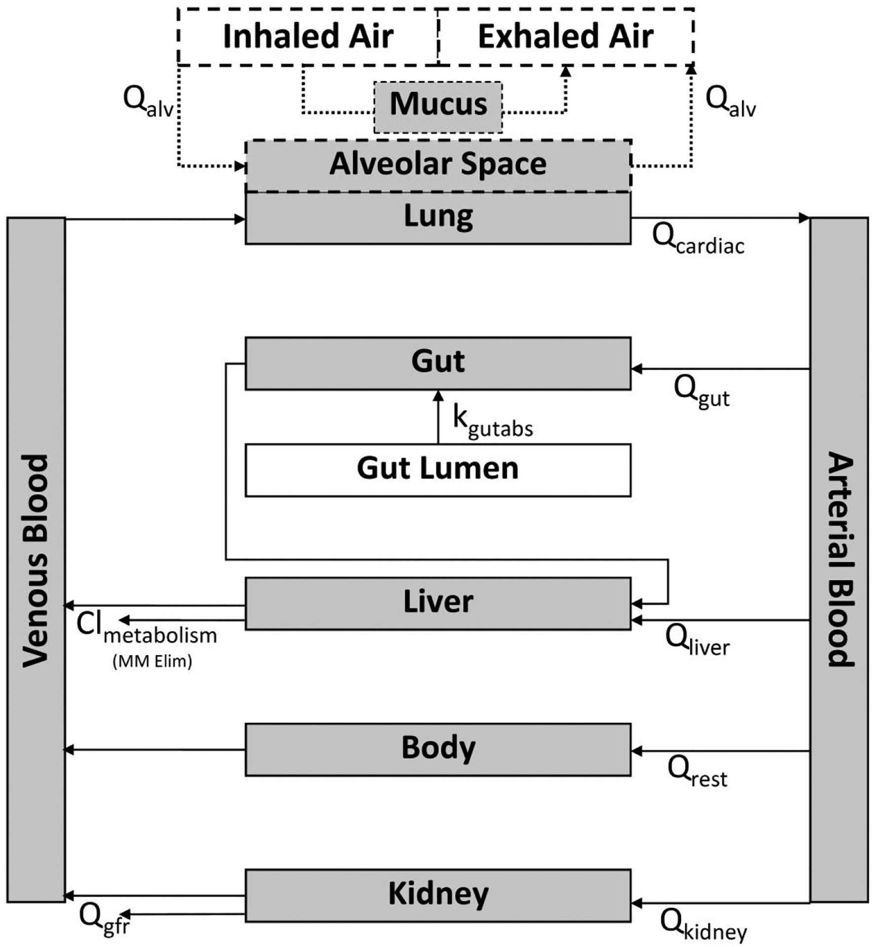
Representation of the httk PBTK model structure with added gas inhalation/exhalation component (dotted lines).

Due to the relatively small number of chemicals used in this investigation, it could not be determined in this study whether comprehensive use of Michaelis-Menten liver metabolism kinetics for all simulation scenarios improves high-throughput simulation estimates as compared to first-order metabolism kinetics. Therefore a user-defined logical was implemented which allows Michaelis-Menten liver metabolism (using user-input V_max and K_m values) when the logical flag is set to ‘TRUE’ by the user. Mass balance was confirmed upon finalization of the model structure.

Model Evaluation

Evaluations were first performed by comparing actual concentration-time values for rat and human exposures to simulations run using the same exposure parameters (air concentration and exposure length) as the studies from which the observed data were obtained (see Table S2 for the studies included). Concentrations (blood, plasma, and exhaled breath) and other measures of internal exposure (C_max and AUC) were log-transformed in order to improve visualization of the data. The log-transformed observed versus simulated concentrations are shown in Figure 2 (Figures S1A–D show the same data, subsetted by species or aggregated sampling matrix). Of note, some data were censored from this evaluation as the observed and/or simulated concentrations were 0 and they disproportionately affected visualization and comparison of these concentrations. Ultimately, 20 datapoints (0.93%) were censored, 7 because there was no chemical detected in the sample (observed concentration = 0) with no reported limit of quantitation and 13 because there were background concentrations at t = 0 (where simulated concentration = 0). The C_max/C_background ratio for the latter category of censored points ranged from 5.2–697.7. A linear regression performed on the log-transformed data had an r² = 0.45 with a slope of 0.46. The RMSE of the log-transformed data against the regression line was 0.76 while the RMSE of the same data directly comparing the simulated and observed values (direct comparison RMSE, e.g. against the line of identity or the prediction that x = y) was 1.11. Approximately 5.1% (2.1% in humans, 3.0% in rats) of the data points analyzed were > 2 orders of magnitude different than expected (0.4% overpredicted and 4.7% underpredicted). In consideration of a more stringent criteria related to the standard uncertainty factor for toxicokinetics,(38) however, approximately 37.5% (22.9% in humans, 14.6% in rats) of the simulated values were > 0.5 orders of magnitude (3.16-fold) different than expected (16.6% overpredicted and 20.9% underpredicted). Trends in data fit were somewhat different for human (slope = 0.49, direct comparison RMSE = 0.92) or rat (slope = 0.36, direct comparison RMSE = 1.33) data. Figure 3 shows the distribution of the difference between log-transformed observed and simulated concentrations for each chemical/species/matrix combination aggregated by Computer-Aided Management of Emergency Operations (CAMEO) chemical class.(39) The largest number of datapoints with 2 log-orders of difference occurred in the final time quartile of the sampling time periods (Figure S2A), though there was no evidence of any trends in observed vs. simulated concentration differences related to molecular weight (Figure S2B), lipophilicity (Figure S2C), or solubility (Figure S2D). Of 33 chemicals with human blood:air partition coefficients available in the literature (see Table S1), 3 (9.1%) had calculated P_BA values over an order of magnitude different than the literature value (Figure S3). To ensure that inclusion of the URT scrubbing component was not superfluous, the analysis was re-run without this component, which resulted in an evident worsening of model fit parameters including a reduction of r² from 0.45 to 0.39 and an increase of RMSE from 1.11 to 1.26.

Figure 2:

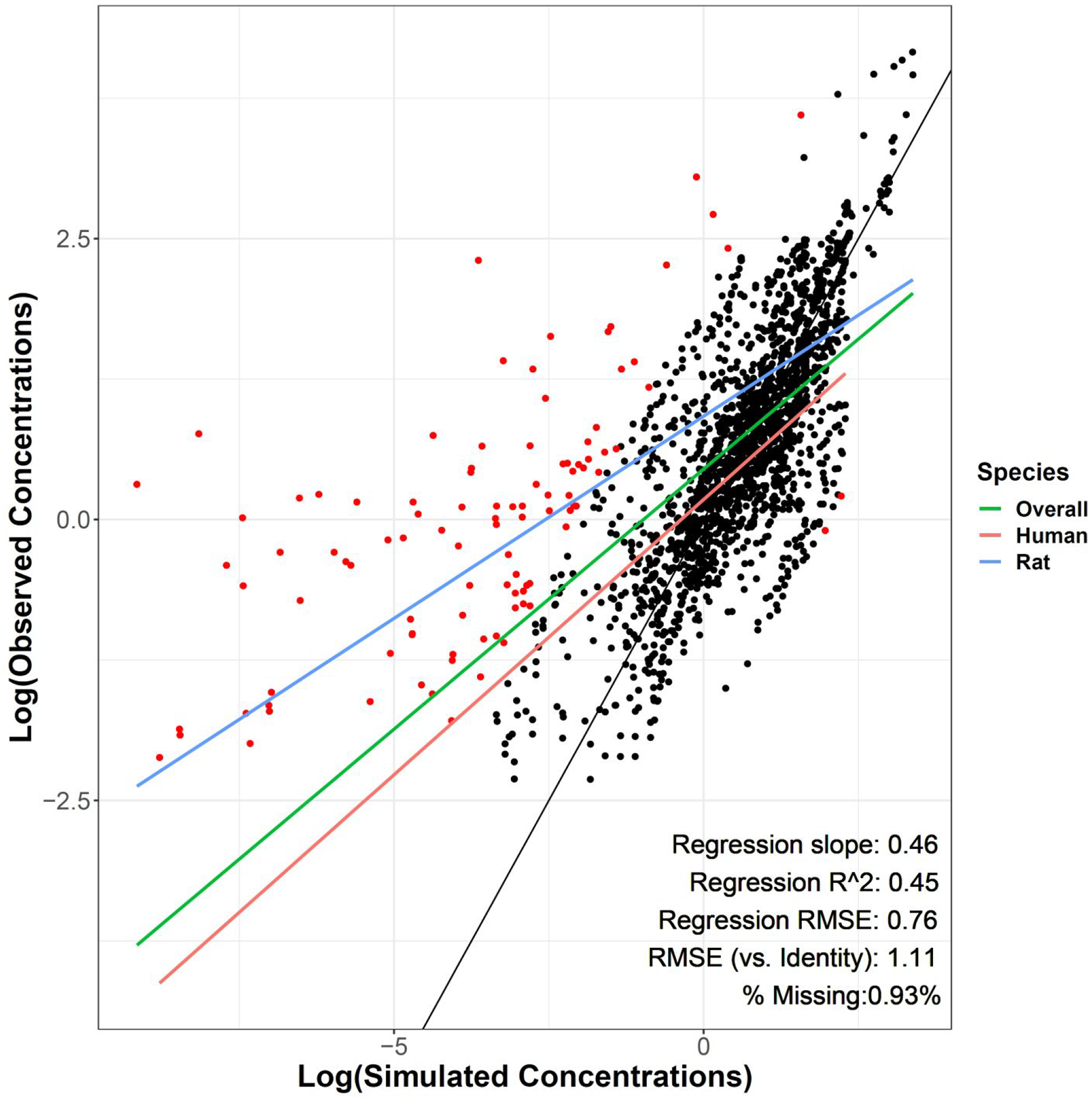
Log-transformed observed (y-axis) vs. simulated (x-axis) blood (μM) and exhaled air (ppm) concentrations. Regression measures of fit are related to the “Overall” regression. Black line is the line of identity (x = y). Red points are >2 log-orders different between observed and simulated values. For visualization purposes, about 0.93% (n = 20) of measured data points were censored because observed or simulated values equaled 0.

Figure 3:

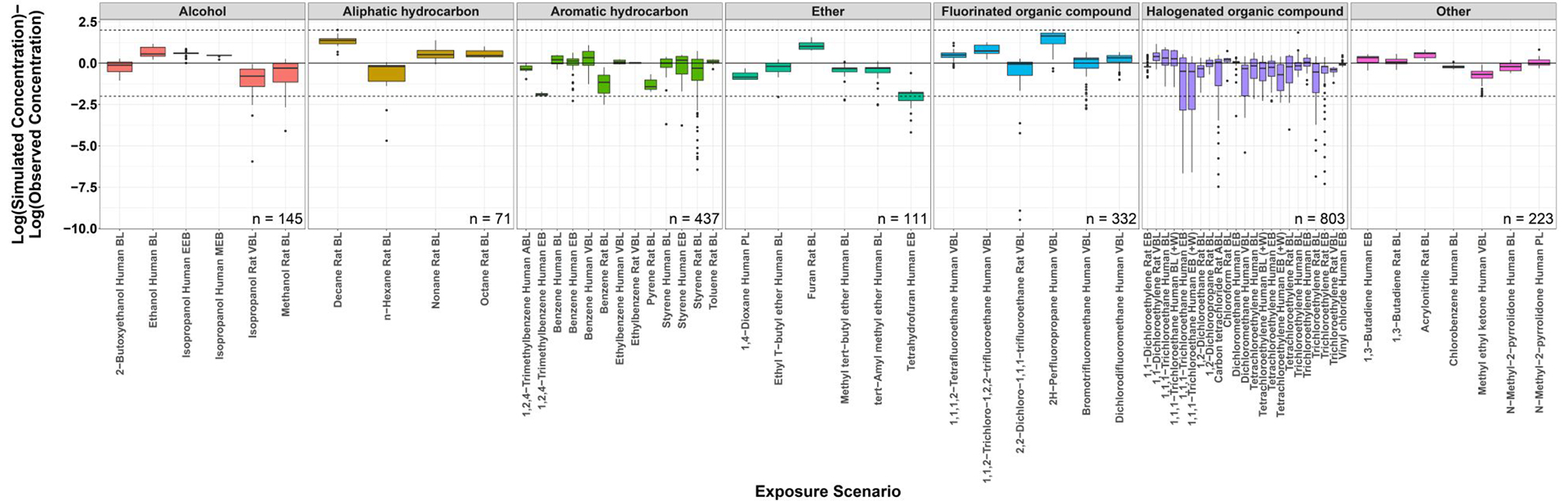
Log-transformed simulated minus observed concentrations for each exposure scenario. Scenarios are grouped by chemical class. Above the zero line indicates model overprediction while below the line indicates underprediction. (BL, Blood; EEB, End-exhaled breath; MEB, Mixed exhaled breath; VBL, Venous blood; ABL, Arterial blood; EB, Unspecified exhaled breath sample (assumed to be EEB); PL, Plasma; +W, with work/exercise).

Further evaluation was done on more aggregated internal exposure measures of maximum concentration (C_max) and area under the concentration-time curve (AUC) (Figures 4A and 4B, broken out by species and matrix in Figures S4A–D and S5A–D). Importantly, in order to compare these log-transformed quantities, any dosing scenarios whose earliest sample collected was after cessation of gas exposure (with a 3% tolerance to allow for inaccuracy in plot digitization, n = 13 dosing scenarios) were not included in this part of the analysis, as C_max and AUC values for these concentration/time curves would not be estimable. For the remaining 129 dosing scenarios, regression r² = 0.67 and 0.79 and slope = 0.88 and 1.02 for log-transformed observed vs. simulated C_max and AUC respectively. The RMSE values for direct comparison of log-transformed simulated and observed values was 0.47 and 0.50. Approximately 5.4% (7 scenarios across 2 chemicals: 2H-perfluoropropane and pyrene) of the log-transformed C_max values and 6.2% (8 scenarios across 4 chemicals: 2H-perfluoropropane, decane, pyrene, and tetrahydrofuran) of the log-transformed AUC values were > 1 order of magnitude different than expected. Here, direct comparison RMSE for observed vs. simulated C_max (human = 0.47, rat = 0.48) and AUC (human = 0.50, rat = 0.50) were relatively similar between species. The sensitivity analysis (Figures S6A and B) demonstrated that the model was generally most sensitive to changes in Log Henry, Log P, and Pulmonary Ventilation Rate values for blood and exhaled breath across most chemical classes. Finally, the results of the individual chemical leave-one-out analysis are shown in Table S3. Several chemicals can be identified from Figures 2–4 as having outlying points (e.g. 2H-perfluoropropane), and, as expected, removing those chemicals in the analysis often resulted in marginally improved slope and RMSE values.

Figures 4.

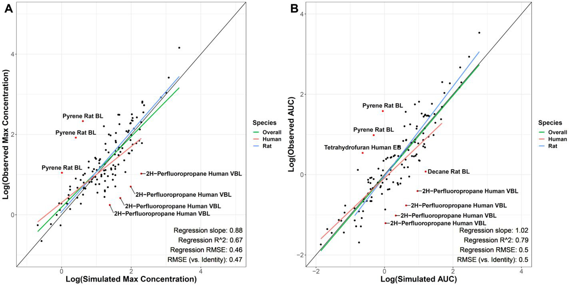
A&B: Log-transformed observed vs. simulated blood and exhaled air max concentrations (A) and area under the curve values (B). Regression measures of fit are related to the “Overall” regression. Black line is the line of identity (x = y). Labeled red points are >1 log-order different between observed and simulated values. (BL, Blood; VBL, venous blood; EB, exhaled breath)

Discussion

This analysis describes the development and examination of a generalized inhalation component for the previously existing httk PBTK model.(12) This model comprises an input inhalation “dose” which is absorbed into the alveolar space, and subsequently, the systemic circulation. Some amount of chemical is additionally exhaled which can be captured as EEB or MEB in the output. A mucus:air partition coefficient also accounts for chemical uptake in the upper respiratory tract. Importantly, this model provided a reasonable simulation of chemical exposures despite never undergoing any optimization. Nonetheless, there were a number of datapoints and chemicals that demonstrated substantial deviation (> 2 orders of magnitude difference) between the observed and simulated values. The RMSE value obtained in this study between observed and predicted concentrations (1.11 on the log scale, indicating a 12.9-fold difference) is greater than the 0.5-log cutoff used in risk assessment applications, however, for a generic model inclusive of >2100 datapoints from exposures to 41 volatile organic chemicals across multiple chemical classes, this level of error indicates a reasonable model fit. Furthermore, the greatest discrepancy between observed and predicted concentrations is seen at later time points (i.e. the last time quartile, Figure S2A) suggesting that the model is doing well at describing absorption/early parts of the concentration time curve, but needs further information and refinement for the elimination/late parts of the curve. Additionally, the RMSEs for C_max (0.47-log) and AUC (0.50-log) were exceptionally close to the 0.5-log cutoff indicating better model fit for these other important pharmacokinetic exposure measures. Though investigations are ongoing, there were no readily apparent trends in which chemicals or chemical properties (e.g. log P, molecular weight, solubility, etc.) were indicators of whether the model would provide a good fit or not. However, sensitivity analysis does suggest that the inhalation model is most sensitive to changes in physicochemical values used to calculate important inhalation partition coefficients, including log P (used to calculate Air:Mucus partition coefficient, Eqn. 4) and Henry’s Law Coefficient (used to calculate Mucus:Air and Water:Air partition coefficients, Eqns. 4 and 3, respectively).

While this is not the first generalized model to describe inhalation exposures to gaseous chemicals, it does provide the additional utility of being readily parameterized by in vitro measures and in silico estimates of chemical properties that are becoming increasingly available (44–46). One previous model on which the present model is heavily based was developed by Jongeneelen et al.(22). That model provides the benefit of being generalizable, with the ability to describe metabolite toxicokinetics and be utilized through a free Microsoft® Excel™ file. While additional chemicals can be added to this detailed model, it is difficult to do so in a high throughput manner. Nonetheless, the Jongeneelen model has the additional benefit of including metabolic products of inhaled chemicals as well as a skin absorption component. Another sophisticated model developed by Ng et al. incorporates a dynamic ventilation piece wherein the ventilation parameters are affected by factors such as exercise or chemical induction.(20) Future efforts will focus on development of a dynamic ventilation option for httk, though because these effects would be so scenario- and chemical-specific, it would likely be added as a user-input option. This functionality would allow the user to adjust ventilation (as was done with two cases in Ng et al.) to better represent any data collected while preserving the generalizability of the model itself. Other similar model building and evaluation efforts have also been published.(25,40)

In addition to integration with a preexisting library for >900 chemicals, another major benefit that the httk model provides in contrast to previous models is that the blood:air partition coefficient can be calculated from physico chemical properties, which can in turn be predicted based solely on the chemical’s structure. This feature allows not only easier high-throughput investigations (P_B:A coefficients do not need to be looked up in literature), but more importantly, it provides the opportunity to run simulations on the thousands of chemicals (with a known structure) that have not yet been investigated to the point of having a literature value for P_B:A. Future integration of httk with open source F_up and CL_INT in silico quantitative property-property relationship (QPPR) based estimators, such as those included in Chebekoue et al.,(41) would make this PBTK model usable for thousands of chemicals without in vitro toxicokinetic data.

Several limitations and assumptions were inherent in this analysis. Firstly, it should be noted that a number of aspects of inhalational physiology were not specifically accounted for in this model. For example, lung metabolism and the presence of lung metabolizing enzymes were not considered for this version of the model. Despite this, the overall goal of this investigation was to generate a generalizable model that was appropriate for a wide variety of chemicals, and though lung metabolism can be exceptionally important in the disposition of certain individual chemicals, it is generally considered to play only a minor role in determining overall bioavailability and distribution of most chemicals.(42) Additionally, modeling of VOC inhalation in isolation is not necessarily representative of the entire system: ingestion and dermal absorption can also play significant roles in the overall absorption of a gaseous chemical.(43) Another important aspect that this model does not yet consider is different exercise or work states. Right now, the model defaults to physiological parameters of individuals “at rest”, but there are numerous instances in which individuals could be exposed to a gaseous chemical while doing light, or even heavy work. As such, implementation of physiological parameters representing different levels of work is a priority future aim in the development of this model. Currently, reactivity in the upper respiratory tract is accounted for with a simple “clearance” constant in the mucus compartment (fit consequences of changing that constant are shown in Table S4). Estimates of actual concentrations may be improved through improvement of the representation of reactivity. Efforts have previously been made to categorize chemicals into “reactive” and “non-reactive” bins which represents a reasonable first step.(44–46) However, QSAR modeling could present an opportunity to quantify the relationship between chemical structure and a “reactivity parameter” that could be included in future models.(47,48) Finally, the current model can only handle exposures to chemicals in the gaseous state. Modeling the inhalation of aerosols and mixtures of aerosols and gases would allow a significantly greater range of occupational exposures to be simulated. The assumption of a single URT compartment made in this study seems to work reasonably well for volatile gases, but a more region-based or even generation-based approach would likely be more appropriate for inhaled aerosols/particles/mixtures.

This model would greatly benefit from a better description of the variability around the simulated concentrations. Both uncertainty and variability of the model can be characterized to allow it to inform chemical risk assessments. Previous work has used techniques including Monte Carlo and global sensitivity analysis to demonstrate the variability associated with population-level estimates,(49,50) but calculation of uncertainty related to underlying physicochemical estimations and model assumptions is also necessary. In particular, population variability in the physiological parameters relevant to inhalation can be simulated by coupling the PBTK model to the “httk-pop” Monte Carlo simulation(50) that infers tissue flows and volumes(51) from the biometrics characterized by the U.S. Centers for Disease Control National Health and Nutrition Examination Survey.(52) Simulating population variability allows the identification of more sensitive populations when “reverse dosimetry”-based in vitro-in vivo extrapolation is used with high throughput in vitro bioactivity screening data.(15,31,50,53,54) Meanwhile, uncertainty in the predictions can be estimated by extrapolating the observed RMSE from the available evaluation data to new chemicals.(19) This extrapolation will presumably be enhanced as additional evaluation data sets across more diverse chemical structures and properties are obtained.(55)

A number of additional gaps and issues also warrant consideration for this model. For example, currently, fat tissue has been aggregated into a “body” compartment that represents all tissues not explicitly broken out in Figure 1. While this reasonably captures the disposition of average chemicals, well-absorbed volatile chemicals tend to skew more lipophilic (consistent with this study where the median log P was 1.96), and will therefore often distribute into the fat to a greater extent.(43) Distribution into and out of a “(rest of) body” compartment, will be simulated to occur (for lipophilic chemicals) faster than it would for an explicit “fat” compartment, which may, in turn, explain the inaccuracies seen in the elimination phase of a number of the chemicals included in this study. In addition, a brain compartment may also improve the utility of the model for consideration of chemicals that act on the brain (i.e. neuroactive chemicals). It should be noted that these compartments can already be split out using the “tissue.data” database built into httk, but they are not included in the PBTK model by default. Another major consideration, which would be more challenging to deal with in a high-throughput manner, is the implementation of metabolite disposition in the model. A number of chemicals (including some of the 41 investigated in this study, like isopropanol) have major metabolites (e.g. acetone) that are just as important from a kinetic and/or activity perspective as the parent compound.(18) In fact, the majority of the simulated points >2 log-orders different from the observed points and the majority of the variability between simulated and observed concentrations came from the final time-quartile of each concentration-time curve (Table S5 and Figure S2A), which indicates an incomplete description of the elimination of chemical from the body. As such, it seems likely that better description of metabolism could potentially, provide better concentration estimates in the last quartile of a concentration-time profile. However, the challenge of implementing a system that could determine what metabolites are needed for a given chemical, and when, in a high-throughput manner would be difficult to solve. That said, there are models under development to provide high-throughput Cytochrome P450 metabolizing enzyme reaction estimations and metabolic stability predictions, which could help drive an overall high-throughput metabolite disposition model.(56–58)

This paper details the design and evaluation of a gas inhalation component for the PBTK model in the httk R package. The described generalizable model can be used to simulate exposures to a broad range of chemicals in a high-throughput manner, provided that an unbound plasma fraction and intrinsic clearance value are available for each chemical.

Supplementary Material

1

Table S1: Information for the 41 chemicals included in the model evaluation and PubMed unique IDs (PMIDs) for the source of metabolism and concentration-time data.

Table S2: List of all exposure scenarios included in the model evaluation.

Table S3: “Leave one out” sensitivity analysis. Table describes the goodness-of-fit parameters for log- transformed data detailed in the results if each of the 41 chemicals is individually left out of the regressions (compare to the top row with “None” left out).

Table S4: Variability in fit slope and Root Mean Square Error (RMSE) vs. identity line with variable upper respiratory tract clearance constant (KurtC) value.

Table S5: List of concentration-time datapoints that had >2 orders of magnitude difference between simulated and observed concentrations.

Figure S1: Log-transformed observed (y-axis) vs. simulated (x-axis) concentrations subsetted by species (A : Human, B: Rat) or sampling matrix (C: Aggregated Exhaled Breath [ppm], D: Aggregated Blood [μM]). Aggregated Exhaled Breath includes all unspecified exhaled breath, end exhaled breath, and mixed exhaled breath samples. Aggregated Blood includes all unspecified blood, venous blood, arterial blood, and plasma samples. Blue line is the regression line of best fit. Black line is the line of identity (x = y). Red points are >2 log-orders different between observed and simulated values.

Figure S2: Log difference between observed and simulated concentrations grouped by time quartile of the concentration-time curve (A), molecular weight (B), log P (C), and solubility (D). Labeled points in S1A are >2 log-orders different between observed and simulated values.

Figure S3: Comparison of experimentally-derived (from literature) and calculated blood:air partition coefficients. Labeled points were > 1 log-order different between experimental and calculated values. Blue line is regression line of best fit with the slope and r² value noted in the bottom. Black line is the line of identity (x = y). RMSE is compared to line of identity.

Figure S4: Log-transformed observed (y-axis) vs. simulated (x-axis) max concentrations subsetted by species (A : Human, B: Rat) or sampling matrix (C: Aggregated Exhaled Breath [ppm], D: Aggregated Blood μM]). Aggregated Exhaled Breath includes all unspecified exhaled breath, end exhaled breath, and mixed exhaled breath samples. Aggregated Blood includes all unspecified blood, venous blood, arterial blood, and plasma samples. Blue line is the regression line of best fit. Black line is the line of identity (x = y). Labeled red points are >1 log-order different between observed and simulated values.

Figure S5: Log-transformed observed (y-axis) vs. simulated (x-axis) area under the concentration-time curve (AUC) subsetted by species (A : Human, B: Rat) or sampling matrix (C: Aggregated Exhaled Breath [ppm], D: Aggregated Blood μM ]). Aggregated Exhaled Breath includes all unspecified exhaled breath, end exhaled breath, and mixed exhaled breath samples. Aggregated Blood includes all unspecified blood, venous blood, arterial blood, and plasma samples. Blue line is the regression line of best fit. Black line is the line of identity (x = y). Labeled red points are >1 log-order different between observed and simulated values.

Figure S6: Sensitivity analysis for input quantities used to calculated model-relevant inhalation values (e.g. Qalv, Kblood2air, Kmuc2air) grouped by A) sampling matrix alone (EB, exhaled breath, end exhaled breath, mixed exhaled breath; BL, blood, arterial blood, venous blood, plasma) or B) sampling matrix and chemical class. GFR, glomerular filtration rate; CLint, intrinsic clearance; Funbound, fraction unbound in plasma; URT, upper respiratory tract.

References

- 1.Scialla M It could take centuries for EPA to test all the unregulated chemicals under a new landmark bill [Internet]. PBS NewsHour. 2016. [cited 2019 Feb 21]. Available from: https://www.pbs.org/newshour/science/it-could-take-centuries-for-epa-to-test-all-the-unregulated-chemicals-under-a-new-landmark-bill [Google Scholar]
- 2.National Toxicology Program. About NTP [Internet]. [cited 2019 Feb 21]. Available from: https://ntp.niehs.nih.gov/about/index.html
- 3.Housenger J Letter to Stakeholders on EPA Office of Pesticide Programs’s Goal to Reduce Animal Testing from Jack E. Housenger, Director Office of Pesticide Programs. [Internet]. Regulations.gov - Supporting & Related Material Document. [cited 2019 Feb 21]. Available from: https://www.regulations.gov/document?D=EPA-HQ-OPP-2016-0093-0003 [Google Scholar]
- 4.Bessems JG, Loizou G, Krishnan K, Clewell HJ, Bernasconi C, Bois F, et al. PBTK modelling platforms and parameter estimation tools to enable animal-free risk assessment: recommendations from a joint EPAA--EURL ECVAM ADME workshop. Regul Toxicol Pharmacol RTP. 2014. Feb;68(1):119–39. [DOI] [PubMed] [Google Scholar]
- 5.Boyes WK, Bercegeay M, Krantz T, Evans M, Benignus V, Simmons JE. Momentary brain concentration of trichloroethylene predicts the effects on rat visual function. Toxicol Sci Off J Soc Toxicol. 2005. September;87(1):187–96. [DOI] [PubMed] [Google Scholar]
- 6.Brochot C, Toth J, Bois FY. Lumping in pharmacokinetics. J Pharmacokinet Pharmacodyn. 2005. Dec;32(5–6):719–36. [DOI] [PubMed] [Google Scholar]
- 7.Nestorov IA, Aarons LJ, Arundel PA, Rowland M. Lumping of whole-body physiologically based pharmacokinetic models. J Pharmacokinet Biopharm. 1998. Feb;26(1):21–46. [DOI] [PubMed] [Google Scholar]
- 8.Gueorguieva I, Nestorov IA, Rowland M. Reducing whole body physiologically based pharmacokinetic models using global sensitivity analysis: diazepam case study. J Pharmacokinet Pharmacodyn. 2006. Feb;33(1):1–27. [DOI] [PubMed] [Google Scholar]
- 9.Clewell RA, Clewell HJ. Development and specification of physiologically based pharmacokinetic models for use in risk assessment. Regul Toxicol Pharmacol RTP. 2008. February;50(1):129–43. [DOI] [PubMed] [Google Scholar]
- 10.Rowland MA, Perkins EJ, Mayo ML. Physiological fidelity or model parsimony? The relative performance of reverse-toxicokinetic modeling approaches. BMC Syst Biol. 2017. 11;11(1):35. [DOI] [PMC free article] [PubMed] [Google Scholar]
- 11.Clark LH, Setzer RW, Barton HA. Framework for evaluation of physiologically-based pharmacokinetic models for use in safety or risk assessment. Risk Anal Off Publ Soc Risk Anal 2004. Dec;24(6):1697–717. [DOI] [PubMed] [Google Scholar]
- 12.Pearce RG, Setzer RW, Strope CL, Wambaugh JF, Sipes NS. httk: R Package for High-Throughput Toxicokinetics. J Stat Softw. 2017. Jul 17;79(4):1–26. [DOI] [PMC free article] [PubMed] [Google Scholar]
- 13.Wambaugh J, Pearce R, Ring C, Honda G, Sfeir M, Davis J, et al. httk: High-Throughput Toxicokinetics [Internet]. 2019. [cited 2019 Oct 18]. Available from: https://CRAN.R-project.org/package=httk
- 14.Pearce RG, Setzer RW, Davis JL, Wambaugh JF. Evaluation and calibration of high-throughput predictions of chemical distribution to tissues. J Pharmacokinet Pharmacodyn. 2017. Dec;44(6):549–65. [DOI] [PMC free article] [PubMed] [Google Scholar]
- 15.Wetmore BA, Wambaugh JF, Allen B, Ferguson SS, Sochaski MA, Setzer RW, et al. Incorporating High-Throughput Exposure Predictions With Dosimetry-Adjusted In Vitro Bioactivity to Inform Chemical Toxicity Testing. Toxicol Sci Off J Soc Toxicol. 2015. November;148(1):121–36. [DOI] [PMC free article] [PubMed] [Google Scholar]
- 16.Wang Y-H. Confidence assessment of the Simcyp time-based approach and a static mathematical model in predicting clinical drug-drug interactions for mechanism-based CYP3A inhibitors. Drug Metab Dispos Biol Fate Chem. 2010. July;38(7):1094–104. [DOI] [PubMed] [Google Scholar]
- 17.Centers for Disease Control and Prevention. NHANES 2013–2014: Volatile Organic Compounds (VOCs) and Trihalomethanes/MTBE - Blood - Special Sample Data Documentation, Codebook, and Frequencies [Internet]. [cited 2019 Feb 21]. Available from: https://wwwn.cdc.gov/Nchs/Nhanes/2013-2014/VOCWBS_H.htm
- 18.Clewell HJ, Gentry PR, Gearhart JM, Covington TR, Banton MI, Andersen ME. Development of a physiologically based pharmacokinetic model of isopropanol and its metabolite acetone. Toxicol Sci Off J Soc Toxicol. 2001. October;63(2):160–72. [DOI] [PubMed] [Google Scholar]
- 19.Cohen Hubal EA, Wetmore BA, Wambaugh JF, El-Masri H, Sobus JR, Bahadori T. Advancing internal exposure and physiologically-based toxicokinetic modeling for 21st-century risk assessments. J Expo Sci Environ Epidemiol. 2019. Jan;29(1):11–20. [DOI] [PMC free article] [PubMed] [Google Scholar]
- 20.Ng LJ, Stuhmiller LM, Stuhmiller JH. Incorporation of acute dynamic ventilation changes into a standardized physiologically based pharmacokinetic model. Inhal Toxicol. 2007. Mar;19(3):247–63. [DOI] [PubMed] [Google Scholar]
- 21.Aylward LL, Kirman CR, Blount BC, Hays SM. Chemical-specific screening criteria for interpretation of biomonitoring data for volatile organic compounds (VOCs)--application of steady-state PBPK model solutions. Regul Toxicol Pharmacol RTP. 2010. Oct;58(1):33–44. [DOI] [PubMed] [Google Scholar]
- 22.Jongeneelen FJ, Berge WFT. A generic, cross-chemical predictive PBTK model with multiple entry routes running as application in MS Excel; design of the model and comparison of predictions with experimental results. Ann Occup Hyg. 2011. Oct;55(8):841–64. [DOI] [PubMed] [Google Scholar]
- 23.Price K, Krishnan K. An integrated QSAR-PBPK modelling approach for predicting the inhalation toxicokinetics of mixtures of volatile organic chemicals in the rat. SAR QSAR Environ Res. 2011. March;22(1–2):107–28. [DOI] [PubMed] [Google Scholar]
- 24.Peyret T, Krishnan K. Quantitative Property-Property Relationship for Screening-Level Prediction of Intrinsic Clearance of Volatile Organic Chemicals in Rats and Its Integration within PBPK Models to Predict Inhalation Pharmacokinetics in Humans. J Toxicol. 2012,’2012:286079. [DOI] [PMC free article] [PubMed] [Google Scholar]
- 25.Mumtaz MM, Ray M, Crowell SR, Keys D, Fisher J, Ruiz P. Translational research to develop a human PBPK models tool kit-volatile organic compounds (VOCs). J Toxicol Environ Health A. 2012;75(1):6–24. [DOI] [PMC free article] [PubMed] [Google Scholar]
- 26.Olie JDN, Bessems JG, Clewell HJ, Meulenbelt J, Hunault CC. Evaluation of semi-generic PBTK modeling for emergency risk assessment after acute inhalation exposure to volatile hazardous chemicals. Chemosphere. 2015. Aug;132:47–55. [DOI] [PubMed] [Google Scholar]
- 27.Sayre R, Wambaugh J, Grulke C. Database of Pharmacokinetic Time-Series Data and Parameters for Evaluating the Safety of Environmental Chemicals. 2019. Apr 22 [cited 2019 May 17]; Available from: https://epa.figshare.com/articles/Database_of_Pharmacokinetic_Time-Series_Data_and_Parameters_for_Evaluating_the_Safety_of_Environmental_Chemicals/8023229 [DOI] [PMC free article] [PubMed]
- 28.Sayre RR, Wambaugh JF, Grulke CM. Database of pharmacokinetic time-series data and parameters for 144 environmental chemicals. (in press). Sci Data. 2020; [DOI] [PMC free article] [PubMed] [Google Scholar]
- 29.Williams AJ, Grulke CM, Edwards J, McEachran AD, Mansouri K, Baker NC, et al. The CompTox Chemistry Dashboard: a community data resource for environmental chemistry. J Cheminformatics. 2017. Nov 28;9(1):61. [DOI] [PMC free article] [PubMed] [Google Scholar]
- 30.Mansouri K, Grulke CM, Judson RS, Williams AJ. OPERA models for predicting physicochemical properties and environmental fate endpoints. J Cheminformatics. 2018. Mar 8;10(1):10. [DOI] [PMC free article] [PubMed] [Google Scholar]
- 31.Wetmore BA, Wambaugh JF, Ferguson SS, Sochaski MA, Rotroff DM, Freeman K, et al. Integration of dosimetry, exposure, and high-throughput screening data in chemical toxicity assessment. Toxicol Sci Off J Soc Toxicol. 2012. January;125(1):157–74. [DOI] [PubMed] [Google Scholar]
- 32.Ito K, Houston JB. Comparison of the use of liver models for predicting drug clearance using in vitro kinetic data from hepatic microsomes and isolated hepatocytes. Pharm Res. 2004. May;21(5):785–92. [DOI] [PubMed] [Google Scholar]
- 33.Schmitt W General approach for the calculation of tissue to plasma partition coefficients. Toxicol Vitro Int J Publ Assoc BIBRA. 2008. Mar;22(2):457–67. [DOI] [PubMed] [Google Scholar]
- 34.Scott JW, Sherrill L, Jiang J, Zhao K. Tuning to odor solubility and sorption pattern in olfactory epithelial responses. J Neurosci Off J Soc Neurosci. 2014. February 5;34(6):2025–36. [DOI] [PMC free article] [PubMed] [Google Scholar]
- 35.Fiserova-Bergerova V Extrapolation of physiological parameters for physiologically based simulation models. Toxicol Lett. 1995. September;79(1–3):77–86. [DOI] [PubMed] [Google Scholar]
- 36.Obach RS. Nonspecific binding to microsomes: impact on scale-up of in vitro intrinsic clearance to hepatic clearance as assessed through examination of warfarin, imipramine, and propranolol. Drug Metab Dispos Biol Fate Chem. 1997. December;25(12):1359–69. [PubMed] [Google Scholar]
- 37.Intagliata S, Rizzo A, Gossman WG. Physiology, Lung Dead Space. In: StatPearls [Internet]. Treasure Island (FL): StatPearls Publishing; 2019. [cited 2019 Jul 1]. Available from: http://www.ncbi.nlm.nih.gov/books/NBK482501/ [PubMed] [Google Scholar]
- 38.Dorne JLCM Renwick AG. The refinement of uncertainty/safety factors in risk assessment by the incorporation of data on toxicokinetic variability in humans. Toxicol Sci Off J Soc Toxicol. 2005. July;86(1):20–6. [DOI] [PubMed] [Google Scholar]
- 39.US EPA O. CAMEO (Computer-Aided Management of Emergency Operations) [Internet]. US EPA. 2013. [cited 2019 Feb 21]. Available from: https://www.epa.gov/cameo
- 40.Emond C, Krishnan K. A physiological pharmacokinetic model based on tissue lipid content for simulating inhalation pharmacokinetics of highly lipophilic volatile organic chemicals. Toxicol Mech Methods. 2006;16(8):395–403. [DOI] [PubMed] [Google Scholar]
- 41.Chebekoue SF, Krishnan K. A framework for application of quantitative property-property relationships (QPPRs) in physiologically based pharmacokinetic (PBPK) models for high-throughput prediction of internal dose of inhaled organic chemicals. Chemosphere. 2019. Jan;215:634–46. [DOI] [PubMed] [Google Scholar]
- 42.Reilly CA, Yost GS. Chapter 10: Sites of Extra Hepatic Metabolism, Part I: Lung In: Pearson PG, Wienkers LC, editors. Handbook of Drug Metabolism [Internet]. 2nd ed 2008. [cited 2019 Feb 21]. Available from: https://www.taylorfrancis.com/ [Google Scholar]
- 43.National Research Council (US) Committee on Contaminated Drinking Water at Camp Lejeune. Contaminated Water Supplies at Camp Lejeune: Assessing Potential Health Effects [Internet]. Washington (DC): National Academies Press (US); 2009. [cited 2019 Feb 21]. Available from: http://www.ncbi.nlm.nih.gov/books/NBK215298/ [PubMed] [Google Scholar]
- 44.US EPA. Methods for Derivation of Inhalation Reference Concentrations and Application of Inhalation Dosimetry (600-8-90-066f) [Internet]. 1994. [cited 2019 Aug 16]. Available from: https://www.epa.gov/sites/production/files/2014-11/documents/rfc_methodology.pdf
- 45.US EPA National Center for Environmental Assessment RTPN, Stanek J Advances In Inhalation Gas Dosimetry For Derivation Of A Reference Concentration (RfC) And Use In Risk Assessment [Internet]. 2012. [cited 2019 Aug 16]. Available from: https://cfpub.epa.gov/ncea/risk/recordisplay.cfm?deid=244650
- 46.Kuempel ED, Sweeney LM, Morris JB, Jarabek AM. Advances in Inhalation Dosimetry Models and Methods for Occupational Risk Assessment and Exposure Limit Derivation. J Occup Environ Hyg. 2015. November 25;12(sup1):S18–40. [DOI] [PMC free article] [PubMed] [Google Scholar]
- 47.Roberts DW. QSAR for upper-respiratory tract irritation. Chem Biol Interact. 1986. March 1;57(3):325–45. [DOI] [PubMed] [Google Scholar]
- 48.Abraham MH, Sanchez-Moreno R, Gil-Lostes J, Acree WE, Enrique Cometto-Muniz J, Cain WS. The biological and toxicological activity of gases and vapors. Toxicol In Vitro. 2010. Mar 1;24(2):357–62. [DOI] [PMC free article] [PubMed] [Google Scholar]
- 49.Wetmore BA, Allen B, Clewell HJ, Parker T, Wambaugh JF, Almond LM, et al. Incorporating population variability and susceptible subpopulations into dosimetry for high-throughput toxicity testing. Toxicol Sci Off J Soc Toxicol. 2014. November;142(1):210–24. [DOI] [PubMed] [Google Scholar]
- 50.Ring CL, Pearce RG, Setzer RW, Wetmore BA, Wambaugh JF. Identifying populations sensitive to environmental chemicals by simulating toxicokinetic variability. Environ Int. 2017;106:105–18. [DOI] [PMC free article] [PubMed] [Google Scholar]
- 51.McNally K, Cotton R, Hogg A, Loizou G. Reprint of PopGen: A virtual human population generator. Toxicology. 2015. June 5;332:77–93. [DOI] [PubMed] [Google Scholar]
- 52.Centers for Disease Control and Prevention (CDC). National Center for Health Statistics (NCHS). National Health and Nutrition Examination Survey Data [Internet]. 2019. [cited 2019 Apr 23]. Available from: https://www.cdc.gov/nchs/nhanes/index.htm
- 53.Tan Y-M, Liao KH, Clewell HJ. Reverse dosimetry: interpreting trihalomethanes biomonitoring data using physiologically based pharmacokinetic modeling. J Expo Sci Environ Epidemiol. 2007. Nov;17(7):591–603. [DOI] [PubMed] [Google Scholar]
- 54.Sipes NS, Wambaugh JF, Pearce R, Auerbach SS, Wetmore BA, Hsieh J-H, et al. An Intuitive Approach for Predicting Potential Human Health Risk with the Tox21 10k Library. Environ SciTechnol. 2017. Sep 19;51(18):10786–96. [DOI] [PMC free article] [PubMed] [Google Scholar]
- 55.Sheridan RP, Feuston BP, Maiorov VN, Kearsley SK. Similarity to molecules in the training set is a good discriminator for prediction accuracy in QSAR. J Chem Inf Comput Sci. 2004. Dec;44(6):1912–28. [DOI] [PubMed] [Google Scholar]
- 56.Sayre R, Wambaugh J, Williams A, Grulke C. A public database supporting evidence-based metabolomics [Internet]. 2018. [cited 2019 May 17]. Available from: https://epa.figshare.com/articles/A_public_database_supporting_evidence-based_metabolomics/7056233
- 57.Tian S, Djoumbou-Feunang Y, Greiner R, Wishart DS. CypReact: A Software Tool for in Silico Reactant Prediction for Human Cytochrome P450 Enzymes. J Chem Inf Model. 2018. Jun 25;58(6):1282–91. [DOI] [PubMed] [Google Scholar]
- 58.Podlewska S, Kafel R. MetStabOn-Online Platform for Metabolic Stability Predictions. Int J Mol Sci 2018. March 30;19(4). [DOI] [PMC free article] [PubMed] [Google Scholar]
Associated Data
This section collects any data citations, data availability statements, or supplementary materials included in this article.
Supplementary Materials