Abstract
The Long Short-Term Memory (LSTM) network is widely used in modeling sequential observations in fields ranging from natural language processing to medical imaging. The LSTM has shown promise for interpreting computed tomography (CT) in lung screening protocols. Yet, traditional image-based LSTM models ignore interval differences, while recently proposed interval-modeled LSTM variants are limited in their ability to interpret temporal proximity. Meanwhile, clinical imaging acquisition may be irregularly sampled, and such sampling patterns may be commingled with clinical usages. In this paper, we propose the Distanced LSTM (DLSTM) by introducing time-distanced (i.e., time distance to the last scan) gates with a temporal emphasis model (TEM) targeting at lung cancer diagnosis (i.e., evaluating the malignancy of pulmonary nodules). Briefly, (1) the time distance of every scan to the last scan is modeled explicitly, (2) time-distanced input and forget gates in DLSTM are introduced across regular and irregular sampling sequences, and (3) the newer scan in serial data is emphasized by the TEM. The DLSTM algorithm is evaluated with both simulated data and real CT images (from 1794 National Lung Screening Trial (NLST) patients with longitudinal scans and 1420 clinical studied patients). Experimental results on simulated data indicate the DLSTM can capture families of temporal relationships that cannot be detected with traditional LSTM. Cross-validation on empirical CT datasets demonstrates that DLSTM achieves leading performance on both regularly and irregularly sampled data (e.g., improving LSTM from 0.6785 to 0.7085 on F1 score in NLST). In external-validation on irregularly acquired data, the benchmarks achieved 0.8350 (CNN feature) and 0.8380 (with LSTM) on AUC score, while the proposed DLSTM achieves 0.8905. In conclusion, the DLSTM approach is shown to be compatible with families of linear, quadratic, exponential, and log-exponential temporal models. The DLSTM can be readily extended with other temporal dependence interactions while hardly increasing overall model complexity.
Keywords: Lung Cancer Diagnosis, Longitudinal, Distanced LSTM, Temporal Emphasis Model
Graphical Abstract
1. Introduction
Lung cancer was estimated as the most common cancer of death in the United States of 2019 (Siegel et al., 2019), and early diagnosis and timely treatment with low-dose computed tomographic (CT) can reduce mortality by over 20% (Aberle et al., 2011). With large data archives and advanced computing resources, deep-learning-based methods have become prevalent techniques in medical image analysis (MIA). Lung cancer diagnosis, as a subset of MIA, has been explored with deep learning methods (Liao et al., 2019)(Ardila et al., 2019)(van Ginneken et al., 2010). From a machine learning perspective, the ultimate objective of the lung cancer diagnosis is to estimate if a patient has lung cancer or not.
The leading automatic lung cancer diagnosis pipeline usually includes two steps: detecting the suspicious pulmonary nodules and analyzing their malignancy. Zhu et al. (Zhu et al., 2018a) introduced the Faster RCNN with 3D dual-path blocks to learn nodule features. DeepSEED (Li et al., 2019) developed a 3D CNN with an encoder-decoder structure for detecting nodules and extensively evaluated on public datasets. Beyond the nodule-based analysis, researchers have explored the lung cancer diagnosis on scan-level or patient-level. Liao et al. (Liao et al., 2019) developed a 3D deep leaky noise-or network, which included nodule detection and classifying the whole lung. Drdila et al. (Ardila et al., 2019) utilized the current and prior CT images as multi-channel input to predict the risk of lung cancer. Wang et al. (Wang et al., 2019) collaboratively used the CT images and clinical demographics for patient-level lung cancer diagnosis. Gao et al. (Gao et al., 2020b) developed a multi-task network for prediction of lung cancer and cancer-free progression. In this paper, our algorithm employed the (Liao et al., 2019) as the feature extraction method, which won the first place in the Kaggle DSB2017 challenge (https://www.kaggle.com/c/data-science-bowl-2017). A limitation of this previous work (Liao et al., 2019) is that the network focuses on single CT scan for each patient and does not take advantage of multiple longitudinal CT scans.
Longitudinal lung screening CT scans contain temporal relevant diagnostic information for lung cancer, and its effectiveness has been explored (e.g., (Ardila et al., 2019)(Xu et al., 2019)). As lung screening is becoming more common, longitudinal lung CT scans are also becoming readily available for decision making in clinical practice. The guidelines for lung screening indicate annual imaging for high-risk patients (https://medlineplus.gov/lungcancer.html). However, in general practice, clinical screening is rarely precisely annual since patients may miss visits or may have less frequent scans due to competing factors. Additionally, if clinical concerns arise, more frequent scans may be possible. In our experiments, longitudinal CT scans are best modeled as irregularly sampled, which indicates the time interval between CT scans varies substantially. As the example shown in Figure 1, a benign nodule can exhibit substantial variations if the time interval is large, while the malignant nodule may vary little within a short time. Hence, careful consideration of the time interval is necessary to provide the context of the different signal between scans. This confounding factor challenges most of learning models (including canonical sequential models) that do not consider the precise timing of scans.
Fig. 1.
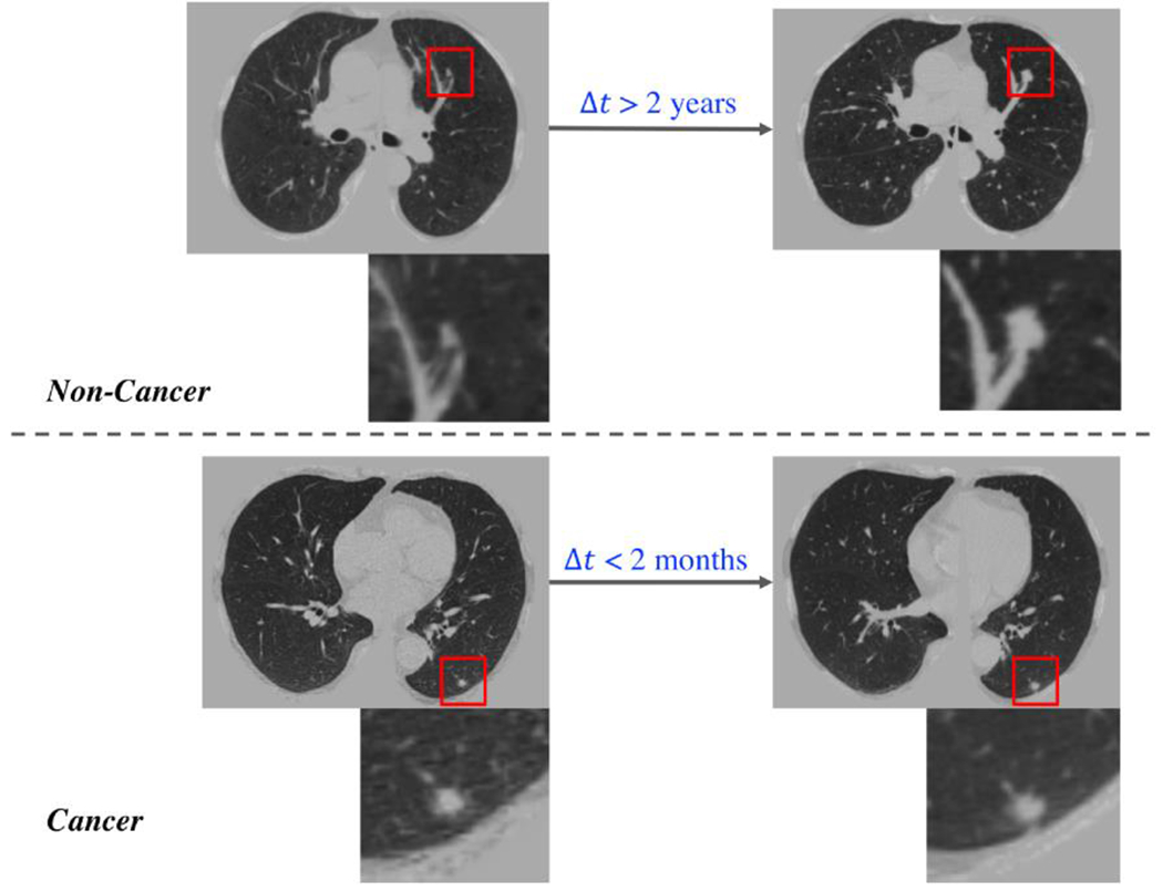
Challenging examples for conventional LSTM. One high-risk region per image is enlarged. The upper CT images are from a cancer-free patient, where the clear changes can be seen in nodule over 2 years. The lower CT images come from a cancer patient, where a clear difference is hard to be visualized within a short time interval.
Recurrent Neural Networks (RNNs) are leading methods to apply deep learning to longitudinal data (e.g., natural language processing (Wen et al., 2015), speech recognition (Han et al., 2017), computer vision (Finn et al., 2006)(Lotter et al., 2016), and medical imaging (Xu et al., 2019)(Santeramo et al., 2018)(Gao et al., 2020a)). Some works (Gregor et al., 2015)(Chung et al., 2015)(Bayer and Osendorfer, 2014) collaborate the RNNs with generative models. The Long Short-Term Memory (LSTM) (Hochreiter and Schmidhuber, 1997) network is a RNN approach that captures both long-term and short-term dependencies within sequential data by introducing the cell state and three gates (i.e., input gate, forget gate and output gate). The LSTM is widely applied to multiple fields including temporal action recognition (Zhu et al., 2016) and pulmonary nodule detection with 3D CNN (Zhu et al., 2018b). Many variants of LSTM have been proposed. Peephole LSTM (Gers and Schmidhuber, 2000) adds a “peephole connection” that allows the gate layers have wider receptive field. The Gated Recurrent Unit (Cho et al., 2014) combined the input gates and forget gates as a single “gate”. Phased LSTM (Neil et al., n.d.) included a new gate with three different phases to address event-based sequential data. Recently, the temporal intervals have been modeled in LSTM (e.g., recommendation system in finance (Zhu et al., 2017) and abnormality detection with 2D chest X-ray (Santeramo et al., 2018)). However, no previous studies have been conducted to model global temporal variations and emphases to the best of our knowledge. The previous methods (Santeramo et al., 2018)(Zhu et al., 2017) have modeled the relative intervals between consecutive scans. However, these methods did not include the global time information.
In this paper, the Distanced LSTM (DLSTM) is proposed to perform lung cancer diagnosis using the longitudinal imaging features from lung CT scans. The novelty of this approach arises from a new Temporal Emphasis Model (TEM) to capture the global time distance from the previous time stamp scan to the last time point. The TEM is aggregated with forget gate and input gate to emphasize more recent scans.
Experiments on simulated data and CT datasets are included to evaluate our method. First, the toy dataset is simulated and termed as Tumor-CIFAR, which is generated by adding dummy nodules to CIFAR10 (Krizhevsky, 2009) according to (Duhaylongsod et al., 1995) that the malignant nodules grow ~3 times faster than benign ones. The performance on Tumor-CIFAR highly supports that our DLSTM can capture the time stamp information in sequences. Second, we include three empirical lung screening CT scan datasets (the National Lung Screening Trial (NLST) (N.L.S.T.R.T.J., 2011), the Vanderbilt Lung Screening Program (VLSP) (https://www.vumc.org/radiology/lung) and the Molecular Characterization Laboratories (MCL) (https://mcl.nci.nih.gov)) including regular and irregular sampled scans. The MCL and VLSP are combined as our in-house dataset.
This paper is the extension of the conference version (Gao et al., 2019). Specifically, we (1) generalize and evaluate the DLSTM (Gao et al., 2019) with four temporal emphasis models and (2) include more comprehensive baseline methods and deeper analyses. In summary, the contributions of this manuscript are:
The proposed DLSTM models the global temporal variations and emphasizes newer scan.
The TEM model is proposed to encode temporal information with the forget gate and input gate in LSTM families.
The evaluations of simulated datasets and three empirical datasets (including cross-validation and external-validation) are provided.
2. Theory
2.1. Task Description and Intuition
Given a set of patients P = {p1, p2, … pn} with longitudinal CT scans, the aim of the network is to predict a label for each patient to indicate whether the patient has cancer or not. For simplification, the following definitions are provided. Each patient pi has m+1 longitudinal scans with data features {X0, … , Xm} from scan acquisition times {T0, … , Tm}. The time intervals between scans {l0, …, lm−1} are computed by lt = Tt+1 − Tt. The time interval to last scan {d0, … , dm} is computed by dt = max{T} − Tt. In this scenario design, dm = 0.
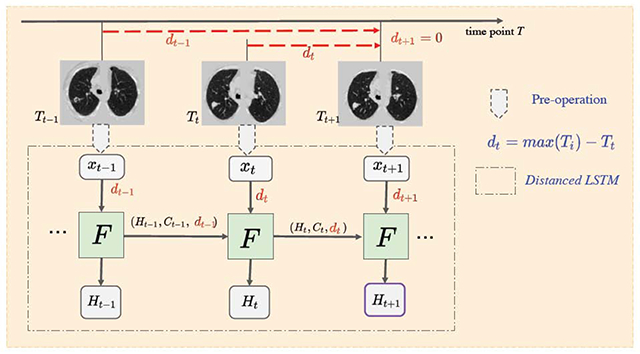
The motivating idea is to model longitudinal data in the context of LSTM. While long term patterns are often of high importance in natural longitudinal learning (e.g., on natural language, voice, videos), we observe that recent scans may detect an event on onset in medical imaging. Two concerns should be addressed for the longitudinal CT scans for diagnosis (1) newer data usually bring more information for diagnosis and (2) timestamp interval information should be included (as shown in Figure 1). Therefore, the time distances of scans are introduced as {dt}, which allow emphasis on the more recent data and also encode the time interval information, in the proposed method (as shown in Figure 2).
Fig. 2.
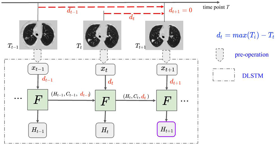
The framework of DLSTM (three “steps” in the example). The pre-operation can be image preprocessing or a feature extraction network. xt is the input data at time point t, and dt is the time distance from the time point t to the latest time point. “F” represents the learnable DLSTM component (convolutional version in this paper). Ht and Ct are the hidden state and cell state, respectively. The input data, xt, could be ID, 2D, or 3D. The last step’s output (e.g., Ht+1) is the output of DLSTM.
2.2. Convolutional LSTM
Convolutional LSTM (Shi et al., 2015) was proposed to integrate LSTM with computer vision tasks (Finn et al., 2006)(Lotter et al., 2016)(Cai et al., 2017). The example of convolutional LSTM (Shi et al, 2015) is used to introduce the core ideas of LSTM family. The LSTM includes three gates (i.e., forget gate, input gate and output gate) and two state units (hidden state and cell state). The whole convolutional LSTM model is provided as:
| (1) |
| (2) |
| (3) |
| (4) |
| (5) |
The input gate it controls information updated, and the forget gate controls the information from cell state for next iteration. The output is based on the cell state filtered by an output gate ot. The cell state keeps the long-term dependency, and the hidden state ht contributes to next step for computing gates and cell state. The weight W and the bias b are the learnable parameters. xt is the input at the time point t. The “*” and “∘” denote the convolution operator and Hadamard product, respectively. The “σ” is the sigmoid function to normalize the gates (i.e., it, ft and ot) to the range of (0,1). The “tanh” represents hyperbolic tangent, which has the range (−1, 1).
Zhu et al. (Zhu et al., 2017) proposed the Time-LSTM, which added a time-interval based gate to LSTM with better modeling user behavior in a recommender system. Santeramo et al. (Santeramo et al., 2018) included an additive term with time interval information in LSTM equations, which was proposed for abnormalities detection of chest X-ray. We employ (Zhu et al., 2017)(Santeramo et al., 2018) as the benchmark methods in this study since those are the most representative time modulated algorithms. Note that for clarity in the remainder of this manuscript, LSTM implicitly refers to convolutional LSTM.
2.3. Distanced LSTM
LSTM family is the most widely used RNNs in classification/prediction with sequential data. The input gate it and forget gate ft are designed to control the information to be stored and forgotten at step Tt and before step Tt, respectively. In classical LSTM, the time points are treated as uniform distribution without modeling the time intervals.
Herein, a focusing term is introduced into the DLSTM method by proposing a Temporal Emphasis Model (TEM). The TEM encodes the time distance dt with a parameter learnable mathematical function. In this paper, four different variations of the DLSTM are introduced as:
| (6) |
| (7) |
| (8) |
| (9) |
where a and c are positive learnable parameters. ε is a small positive value without prior knowledge. D(dt, a, c) represents the TEM in the following.
The proposed TEM model is multiplied with the input gate and forget gate in LSTM. Here, we follow the equations (1–5) to form the DLSTM:
| (10) |
| (11) |
| (12) |
| (13) |
| (14) |
Since the input gate handles the current step t, the TEM model encodes current time distance dt into D(dt, a, c) to form the time-distanced input gate it. The forget gate multiplies the TEM model D(dt-1, a, c) at time t − 1 because the forget gate ft addresses the “previous” information.
3. Method
3.1. Simulation: Tumor-CIFAR
First, we examine the asymptotic performance of the temporal learning models as the datasets become large. Here, simulations provide both scalability and certain ground truth.
3.1.1. Dataset
The public CIFAR10 dataset (Krizhevsky A, Hinton G, 2009) contains 60,000 natural images with size of 32 × 32, across highly heterogenous classes. It is widely used to evaluate methods while requiring minimal efforts on preprocessing and computing (given the small image size). In our simulation, each image in CIFAR10 has been extended to five sequential images with two gradually growing nodules, as shown in Figure 3. The nodule size si is computed by
where ti is the time stamp from the beginning point, g is the growth rate, i is the sequential index. The difference between malignant and benign nodules is the growth rate g. We follow the finding of (Duhaylongsod et al., 1995.), that the growth rate of malignant pulmonary nodules is approximately three times as the benign one. The growth rate g of simulated nodules is
| 15) |
where N(μ, σ2) represents the Gaussian distribution with μ as mean and σ2 as variance. Thus, the classification of malignant and benign nodules is transferred to classification of growth rate, which is computed by nodule size and time information . The simulation code, detail generating descriptions and more image examples are publicly available at https://github.com/MASILab/tumor-cifar.
Fig. 3.
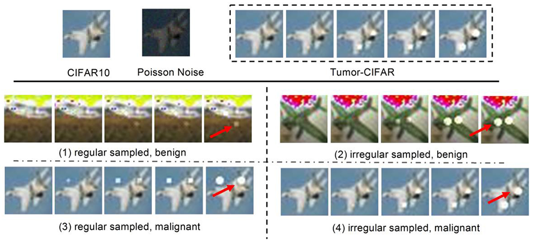
Illustration of the Tumor-CIFAR. The upper panel shows the differences between CIFAR10 and Tumor-CIFAR. Each image in CIFAR10 will be transformed into a five-step longitudinal sample by adding growing nodules and Poisson noise (the intensities of noise map in the figure are magnified ten times for better visualization). The bottom panel show more examples in the two version datasets we simulated (e.g., nodules are added to ‘airplane’). The bottom-left panel is from version 1, which has the same time interval distribution, different nodule sizes between benign and malignant. The bottom-right panel is from version 2, which has the same nodule size distribution, different time intenvals between benign and malignant, the dummy nodules are shown as white blobs (some are indicated by red arrows).
Motivated by (Boas and Fleischmann, 2012) that Poisson noise is one of the prevalent noises in CT imaging, Poisson noise (intensities of noise map are linearly normalized to 0-10) is added to the Tumor-CIFAR. Another implementation of adding salt and pepper noise can be found in the public GitHub repository.
We study two applications of the DLSTM model here with two versions of the Tumor-CIFAR.
Regular Sampled (version 1): the image samples have the same “interval distribution” but different nodule “size distribution” between benign and malignant (bottom left panel of Figure 3).
Irregular Sampled (version 2): the same nodule “size distribution” but different “interval distribution” between benign and malignant (bottom right panel of Figure 3).
The Regular Sampled version is designed to verify if the emphasis on different scans will be helpful for classification when the time interval is under the same distribution for benign and malignant (rough regularly sampled). The Irregular Sampled version, with extremely irregularly sampled (e.g the time interval can differ more than 2 times across subjects) data, measures if our method can capture the time distance difference between the malignant and benign samples.
3.1.2. Experimental Design
There are 50,000 training samples and 10,000 test samples in Tumor-CIFAR. Each sample has 5 sequential images as longitudinal data. The simulated malignant prevalence is 50% in both training and test sets, and the training set is further randomly split into training and validation as 4:1.
The base network structure (CNN in results Figure 7), termed as “ToyNet”. is borrowed from the official example for MNIST of PyTorch 0.41 (Paszke et al. 2019). The ToyNet contains two convolutional layers (a 2D dropout after the second) and followed by two fully connected layers along with a ID dropout layer in the middle. The methods “LSTM” and “DLSTM” in Figure 7 represent the 2D convolutional LSTM and 2D convolutional DLSTM stacked in the beginning of the ToyNet, respectively. Training parameters are illustrated in Table 1. The initial learning rate is set as 0.01 and is multiplied by 0.4 at 50th, 70th and 80th epochs. 3D RPN and 3DDLNN are the CNNs borrowed from Liao et al. (Liao et al., 2019) to extract scan-level feature.
Fig. 7.
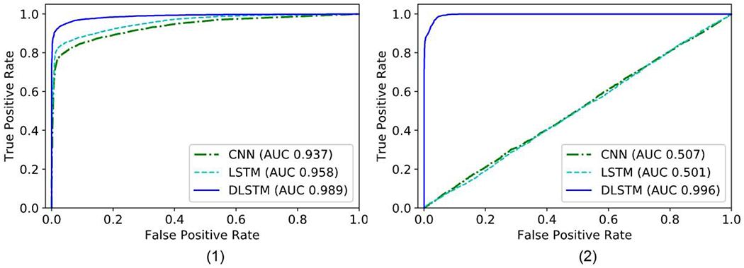
The receiver operating characteristic (ROC) curves of the results on Tumor-CIFAR. The right bottom of the figures shows the Area Under the Curve (AUC) values of different methods. (1) version 1: rough regularly sampled data. The CNN and LSTM achieve reasonable performance, and the proposed DLSTM performs better. (2) version 2: extremely irregularly sampled data. The CNN and LSTM achieve minimal
Table 1.
Training parameters in Tumor-CIFAR and CT datasets
| Initial Learning Rate | Decreased Epochs | Decreased Ratio | Max Epoch | Optimizer | Weight Decay |
|---|---|---|---|---|---|
| 0.01 | [50, 70, 80] | 0.4 | 100 | Adam | 0 |
3D RPN and 3DDLNN are the CNNs borrowed from Liao et al. (Liao et al., 2019) to extract scan-level feature.
3.2. Empirical Chest CTs
Three different evaluation settings are conducted on empirical chest computed tomography (CT) datasets. (1) cross-validation on longitudinal national lung screening trial (NLST) datasets (which are rough regularly sampled), (2) cross-validation on clinical cohort (including cross-sectional and longitudinal, and largely irregularly sampled data), (3) trained on NLST and test on clinical longitudinal data as external-validation.
3.2.1. Dataset
We include three lung screening CT datasets in this paper: National Lung Screening Trial (NLST), Molecular Characterization Laboratories (MCL) and Vanderbilt Lung Screening Program (VLSP). The demographics of each are shown in Table 2. NLST (N.L.S.T.R.T.J., 2011) is a large-scale randomized controlled trial for early diagnosis of lung cancer with low-dose CT screening exams. From the machine learning perspective, NLST is unbalanced since cancer patients are less frequent than non-cancer patients. We obtain a subset (1794 longitudinal subjects) from NLST, termed as “NLST” in Table 2, which includes all the longitudinal subjects with the label “follow-up confirmed lung cancer” (the ground truth is 1) and a random subset of “follow-up confirmed not lung cancer” longitudinal scans (the ground truth is 0). The in-house datasets VLSP (https://www.vumc.org/radiology/lung) and MCL (https://mcl.nci.nih.gov) are combined as the clinical dataset cohort. These data are used in the de-identified form under internal review board supervision.
Table 2.
Demographic distribution in our experiments
| Lung Data Source | NLST | MCL | VLSP |
|---|---|---|---|
| Total Subject | 1794 | 567 | 853 |
| Longitudinal Subject | 1794 | 105 | 370 |
| Cancer Frequency (%) | 40.35 | 68.57 | 2.31 |
| Gender (male, %) | 59.59 | 58.92 | 54.87 |
3.2.2. Data Preprocessing and Nodule Detection
In terms of lung CT datasets, we follow the data preprocess and nodule detection of Liao et al. (Liao et al., 2019). The CT scans are resampled to 1 × 1 × 1mm3 isotropic resolution, and then the scan is segmented by the open source code (https://github.com/lfz/DSB2017). Briefly, the CT images are first converted to Hounsfield Unit (HU) and the image volumes are normalized by a window of [−1200, 600], The lung masks from (Liao et al., 2019) are used to remove the context outside the lung. The 128 × 128 × 128 volume patches are put into 3D RPN (Ren et al., 2017) to locate the pulmonary nodules as (Liao et al., 2019). The top five highest confidence regions are selected, as shown in Figure 4, for classifying the whole scan.
Fig. 4.
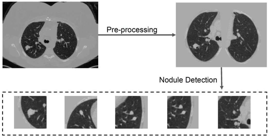
Preprocessing and nodule detection. Both steps follow the open-source code of Liao et al. (Liao et al.. 2019). Briefly, the preprocessing segments the lung and get rid of the background in chest CT, and nodule detection detects five highest risk regions. If the number of detected nodules is less than five, patches of all zeros are added to create the five patches.
3.2.3. Experimental Design
We follow the image preprocessing and nodule detection pipeline of Liao et al. (Liao et al., 2019). Our network can be trained end-to-end, or considered as a lightweight post-processing component. In this section, we evaluate the effectiveness of the proposed method as the postprocessing network.
The pipeline including the CNNs and DLSTM components for chest CTs is shown in Figure 5. The five highest risk regions (possible nodules) for each CT scan are selected by 3D RPN (Ren et al., 2017). After feeding into the pre-trained 3DDLNN model of (Liao et al., 2019), each region is modeled as a ID feature (1x64 vector). The scan-level feature is achieved by concatenating region features into a 5×64 matrix.
Fig. 5.
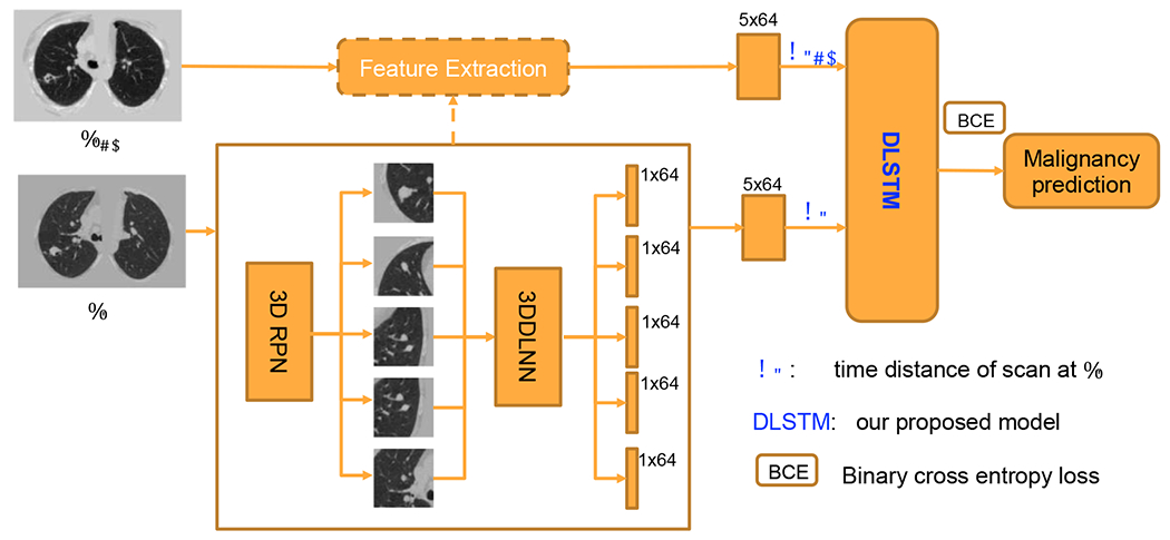
The pipeline for chest CTs. The serial CT images are from the same person at Tt−1 and Tt. The The details of DLSTM and time distance definition dt are illustrated in Figure 2 and Section 2.
Figure 6 presents the experimental design. For a fair comparison, the same features are feed to the Multi-channel CNN (MC-CNN), LSTM, Time-LSTM, tLSTM, and DLSTM networks (see Figure 8). MC-CNN concatenates multi-scan features in the “channel” dimension, which is motivated by the strategy in (Ardila et al., 2019). The LSTM-based methods model the longitudinal data as the sequence. The training parameters are shown in Table 1. Metrics of Accuracy, AUC, F1 score, Recall, Precision are compared. McNemar test has performed combining predicting of five folds. Since CT image data is precious and most lengths of longitudinal steps are less than three, the sequence length in this section is set to two and the last two longitudinal scans are selected.
Fig. 6.
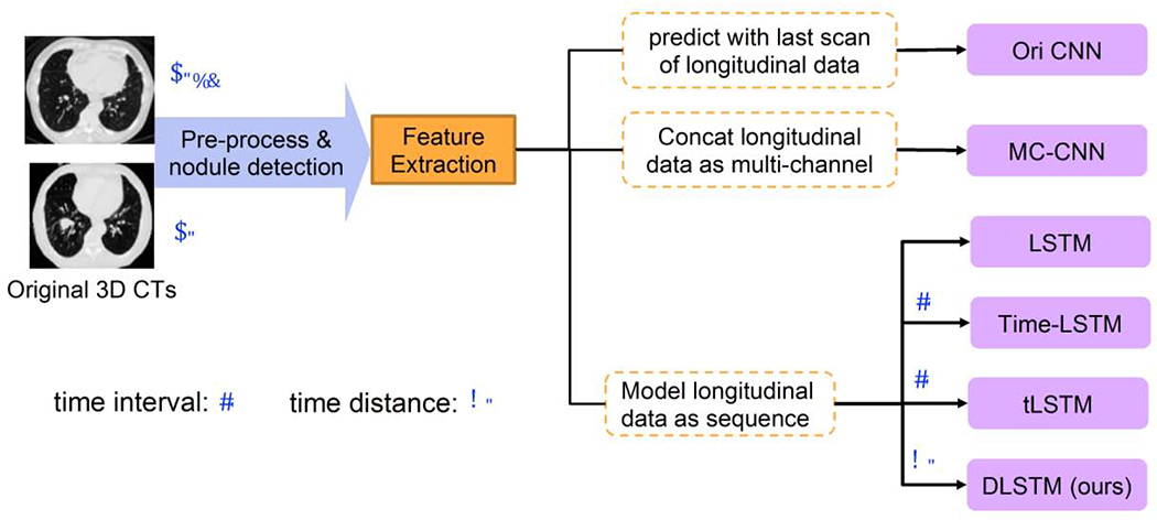
The experimental design of CT images. The 3DDLNN is the network structure from (Liao et al., 2019). Six different methods are compared in our experiments, including two newly time-modeled LSTM algorithms (Time-LSTM (Zhu et al., 2017) and tLSTM (Santeramo et al., 2018)). Those two integrate the time interval lt in the model, while our method introduces the new concept of time distance dt. Please refer to Section 2.1 for the definitions of lt and dt.
Fig. 8.
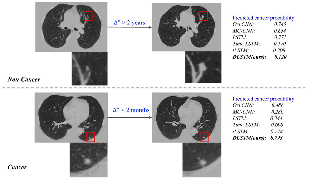
Qualitative results related to Figure 1. The upper part is from a non-cancer patient, which with large time interval between two scans. The bottom part is from a cancer, and the two scans is close at time distance. The DLSTM is the exponential version.
The “Ori CNN” in Tables 3–5 represents the results obtained by open source code and trained model of (Liao et al., 2019). The results are reported at patient-level rather than scan-level. The “Ori CNN” reports the performance of the last scan for each patient. Briefly, we have the following three experimental settings:
Table 3.
Experimental results on NLST dataset (%, average (std) of cross-validation)
| Method | Accuracy | AUC | F1 | Recall | Precision | p-value |
|---|---|---|---|---|---|---|
| Ori CNN | 71.94(2.07) | 74.18(2.11) | 52.18(2.83) | 38.07(2.63) | 83.24(4.24) | <0.05 |
| MC-CNN | 73.26(3.10) | 77.96(0.98) | 59.39(3.70) | 47.91(4.87) | 78.62(3.09) | <0.05 |
| LSTM | 77.05(1.46) | 80.84(1.20) | 67.85(2.41) | 59.92(4.43) | 78.68(3.32) | <0.05 |
| Time-LSTM | 77.91(2.18) | 81.41(0.45) | 69.01(2.85) | 61.16(3.71) | 79.60(4.68) | <0.05 |
| tLSTM | 77.37(2.97) | 80.80(1.45) | 67.47(2.46) | 58.65(5.12) | 79.81(3.34) | <0.05 |
| DLSTM1 | 78.96(1.57) | 82.55(1.31) | 70.85(1.82) | 61.61(2.01) | 83.38(4.34) | *(base) |
| DLSTM2 | 78.63(1.45) | 81.51(1.11) | 68.35(2.03) | 57.49(3.87) | 84.88(4.56) | -- |
| DLSTM3 | 78.68(1.51) | 81.54(0.94) | 68.76(1.78) | 57.76(3.25) | 85.40(4.06) | -- |
| DLSTM4 | 78.05(2.01) | 82.09(1.38) | 68.90(2.52) | 59.84(3.48) | 81.44(3.43) | -- |
The average and standard deviation (std) of five-fold test results are reported.
The best average results are shown in bold. The p < 0.05 indicates our method ing significantly improve the compared method (McNemar test).
Methods citations: Ori CNN (Liao et al.. 2019), LSTM(Hochreiter and Schmidhuber, 1997) (Shi et al., 2015), Time-LSTM (Zhu et al., 2017), tLSTM(Santeramo et al., 2018).
Table 5.
Experimental results on cross-dataset test (%, external-validation)
| Method | Accuracy | AUC | F1 | Recall | Precision | p-value |
|---|---|---|---|---|---|---|
| Train and Test both on longitudinal subjects | ||||||
| Ori CNN (all scans) | 83.42 | 83.50 | 52.53 | 45.77 | 62.66 | <0.05 |
| Ori CNN | 87.58 | 85.10 | 59.31 | 55.13 | 64.18 | <0.05 |
| MC-CNN | 85.89 | 76.54 | 56.21 | 55.13 | 57.33 | <0.05 |
| LSTM | 85.89 | 83.80 | 57.32 | 57.69 | 56.92 | <0.05 |
| Time-LSTM | 88.00 | 87.82 | 65.87 | 68.75 | 63.22 | <0.05 |
| tLSTM | 86.73 | 88.69 | 66.31 | 79.49 | 56.88 | <0.05 |
| DLSTM1 | 88.63 | 89.05 | 68.24 | 74.36 | 63.04 | *(base) |
| DLSTM2 | 89.47 | 88.62 | 69.14 | 70.00 | 68.29 | -- |
| DLSTM3 | 89.47 | 87.39 | 67.11 | 63.75 | 70.83 | -- |
| DLSTM4 | 89.26 | 88.42 | 69.46 | 72.50 | 66.67 | -- |
The best results are shown in bold. The p < 0.05 indicates our method significantly improve the compared method (McNemar test).
Methods citations: Ori CNN (Liao et al., 2019), LSTM(Hochreiter and Schmidhuber, 1997) (Shi et al., 2015), Time-LSTM (Zhu et al., 2017), tLSTM(Santeramo et al., 2018).
Cross-validation on NLST longitudinal scans (setting 1).
We only include the patients with longitudinal scans in NUST and perform cross-validation as shown in Table 3 for 1794 subjects.
Cross-validation on combining cross-sectional and longitudinal scans (setting 2).
As shown in the dataset demographic table (Table 2), more than half of the patients only have a single CT scan (cross-sectional) from the clinical in-house cohort. We duplicate the cross-sectional scans to the dummy “two steps” longitudinal scans. For the time information involved methods (i.e., Time-LSTM, tLSTM, and DLSTM), we set both the time interval and time distance of dummy longitudinal scans to zero.
External-validation on longitudinal scans across data cohorts (setting 3).
To test the generalization ability of our model, we train the model on NLST and test the model on longitudinal clinical data as external validation. The parameter is tuned within the NLST dataset, and then directly applied to the model in longitudinal clinical subjects. Note that the longitudinal data are rough regularly sampled in NLST while the clinical dataset is largely irregular acquired subjects. The NLST dataset is split into five folds (as in setting 1) for training, and the final predicted cancer probability for each subject is the average of five models trained on five folds of NLST when calculating the five metrics.
4. Experimental Results
4.1. Simulation: Tumor-CIFAR
The results of simulation are shown in Figure 7. From Figure 7(1), our DLSTM achieves better results (AUC 0.989) than the baseline methods CNN (AUC 0.937) and LSTM (AUC 0.958) on the regularly sampled (version 1) Tumor-CIFAR. Figure 7(2) shows the experimental results on Version 2 Tumor-CIFAR. The irregularly sampled (version 2) Tumor-CIFAR is an extremely irregularly sampled dataset, whose nodule size distributions are the same between benign and malignant samples. The DLSTM is extremely predictive (AUC 0.996), while the algorithms without time information (CNN and LSTM) achieve minimal discrimination between malignant and benign samples. Our method significantly improves the LSTM and CNN in both version 1 and version 2 (p < 0.05, McNemar test).
4.2. Empirical Chest CTs
The experimental results of setting 1 are shown wn in Table 3. Our methods achieve the highest performances on all five evaluation metrics across the compared methods. Table 4 illustrates the five-fold cross-validation of 1420 clinical subjects (setting 2), and our DLSTM shows competitive results. Table 5 shows the results of external-validation on longitudinal scans (setting 3). The “Ori CNN (all scans)” in Table 5 represents the results computed by all scans of longitudinal subjects independently, and the “Ori CNN” only includes the last scan for each subject.
Table 4.
Experimental results on clinical datasets (%, average (std) of cross-validation)
| Method | Accuracy | AUC | F1 | Recall | Precision | p-value |
|---|---|---|---|---|---|---|
| Ori CNN | 84.80(2.43) | 89.00(1.65) | 70.29(4.26) | 63.46(3.51) | 78.83(5.70) | <0.05 |
| MC-CNN | 84.51(1.29) | 90.85(1.13) | 70.55(1.29) | 62.85(1.53) | 80.84(4.42) | <0.05 |
| LSTM | 86.27(1.29) | 90.27(1.15) | 74.17(2.47) | 69.73(2.62) | 79.56(5.69) | 0.08 |
| Time-LSTM | 85.79(2.37) | 90.81(1.57) | 74.57(3.81) | 71.08(3.56) | 78.71(6.48) | 0.42 |
| tLSTM | 86.42(1.48) | 91.06(1.48) | 74.36(1.99) | 68.55(1.55) | 81.49(5.28) | 0.40 |
| DLSTM1 | 86.97(1.45) | 91.17(1.53) | 76.11(2.68) | 72.71(2.38) | 80.04(5.18) | *(base) |
| DLSTM2 | 86.98(1.20) | 91.41(1.51) | 75.54(1.67) | 71.24(5.01) | 81.22(6.11) | -- |
| DLSTM3 | 85.99(1.13) | 91.10(1.69) | 74.68(2.89) | 70.51(6.07) | 80.23(5.55) | -- |
| DLSTM4 | 86.91(1.37) | 91.07(1.28) | 75.85(1.94) | 72.39(3.65) | 80.21(6.34) | -- |
The average and standard deviation (std) of five-fold test results are reported.
The best average results are shown in bold. The p < 0.05 indicates our method significantly improve the compared method (McNemar test).
Methods citations: Ori CNN (Liao et al., 2019), LSTM(Hochreiter and Schmidhuber, 1997) (Shi et al., 2015), Time-LSTM (Zhu et al., 2017), tLSTM(Santeramo et al., 2018).
We show the qualitative results (Figure 8) in response to the challenge examples in Figure 1. The MC-CNN and LSTM which do not include temporal information, fail in the challenging case. While when time information is included, the algorithms perform better, and our DLSTM achieves superior results.
In both cross-validation and external-validation, our method achieves competitive results across all five metrics including accuracy, AUC, F1 score, recall and precision. In this crossvalidation, our method is empirically evaluated to be effective in the longitudinal subjects set from NLST (setting 1) and clinical datasets combining cross-sectional and longitudinal subjects (setting 2). For example, our proposed DLSTM improves the conventional LSTM on F1 score from 0.6785 to 0.7085 (Table 3, NLST dataset), and from 0.7417 to 0.7611 (Table 4, clinical cohort).
The experiments of external-validation (setting 3) support that the two concerns in Section 2.1 should be addressed: (1) the latest scans achieve higher performance compared with all scans (as Table 4), which supports that the emphasis on last scan is meaningful. (2) The method without time information could be worse than the “Ori CNN” performance, indicating the time-information exclusion may ruin the model in practice. Additionally, our model addresses the two concerns effectively and outperforms the existing time-information included models comprehensively.
5. Discussion
Experiments on Tumor-CIFAR.
The proposed DLSTM (AUC 0.984) outperforms the baselines (i.e., CNN (AUC 0.917) and LSTM (AUC 0.953)) in Tumor-CIFAR-vl, which indicates that the DLSTM can work better on regularly sampled longitudinal data. The results of version 2 indicate that the classification is very challenging for time-free models (i.e., not include the time information and only feed the image) if the longitudinal data is extremely irregularly sampled, while the proposed DLSTM captures the time dependence effectively.
We provide the analytical equation Eq. (15) for prediction (malignant vs. benign) using the lesion size and time stamp in Section 3.1.1 for simulation. In theory, the Eq. (15) can be adopted to assess the growth rate of the pulmonary nodule and then the growth rate can be furtherly applied to predict the nodule malignancy. However, in practice, the exact pulmonary nodule size is usually not available. Also, the indicators of lung cancer are complicated which may not only be evidenced by the nodule size or growth rate. More indicators (such as nodule shape, nodule intensity, tissue around the nodule, nodule location) could also play essential roles. These factors can be indicated by the CT images. Thus, it is hard to directly use an analytical equation in practice that with only considers the pulmonary nodule size and time stamps. However, we believe the size and time can be included as important indicators if the data is available.
Experiments on Lung CT Cohorts.
The traditional CNN network (e.g., (Liao et al., 2019)) only takes one scan per patient for the lung cancer diagnosis, ignoring the additional variations encoded in longitudinal scans. The multi-channel CNN strategy (similar to (Ardila et al., 2019)) concentrates the longitudinal scans at the channel dimension, which does not highlight the time and order information. The LSTM utilizes the order of sequence while overlooking the timestamp of scans. The found time-included methods (e.g., Time-LSTM(Zhu et al., 2017) and tLSTM (Santeramo et al., 2018)) can model the time intervals between consecutive scans, but neglect the global information that newer scans are typically more informative.
Our DLSTM is motivated by the explanation of forget gate and input gate in LSTM. The temporal emphasis model (TEM) in DLSTM is the decrement function taking time distance, indicating the longer distance scan receives less emphasis. The time distances of longitudinal scans include global information, and the local differences (similar as the time interval in (Zhu et al., 2017) (Santeramo et al., 2018)) are encoded by two adjacent time distances. Briefly, our method introduces the explainable time-distanced gates without changing the LSTM structure.
Our proposed method shows significant improvement (p < 0.05) over compared methods under the contexts of longitudinal imaging (setting 1 and 3). Under the setting 2 of cross-validation on combining cross-sectional (single scan per subject) and longitudinal scans, the overall improvements can be indicated by the five metrics, while the p-values indicate that improvement from our method on the LSTM-based methods is not significant. The potential reason is the sequential methods (ours and the compared LSTM-based methods) can be biased by the large ratio (−66%. indicated by Table 2) of cross-sectional scans.
Another interesting finding is the comparison o f the four different backbone functions in the DLSTM. Overall, those models achieve similar performance, indicating that the DLSTM approach is compatible with families of linear, quadratic, exponential, and log-exponential temporal models. In refined comparison, the quadratic version (DLSTM3) achieves the “least satisfying” comprehensive performances, and it is the only concave function among compared backbones. In practice, we would recommend using the convex function as the backbone since the DLSTM1 achieves the most robust performances across different settings and metrics.
Summary.
We propose the novel Distanced LSTM (DLSTM) along with time-distanced gates to model the global temporal intervals between longitudinal CT scans for lung cancer diagnosis. The experiments on the simulated datasets (Tumor-CIFARs) and empirical CT datasets with five metrics (including 1794 NLST and 1420 in-house subjects) demonstrate the effectiveness of DLSTM. Our method is generally superior to baseline methods and the representative existing time-information included methods (i.e., Time-LSTM and tLSTM) under the cross-validation and external-validation settings. The core of DLSTM should be generalizable, indicating that the concept of “time distance” is easy to be extended with other temporal dependence without increasing the model complexity.
Highlights.
Explainable Time-Distanced Gates in LSTM to build Distanced LSTM.
The time distance of every scan to the last scan is modeled explicitly.
The newer scan in serial data is emphasized by our model.
Simulated data and 3 CT datasets including cross-and external-validation.
The document, dataset and the code of simulation are publicly available.
6. Acknowledgements
This research was supported by NSF CAREER 1452485 and R01 EB017230. This study was supported in part by a UO1 CA196405 to Massion. This study was in part using the resources of the Advanced Computing Center for Research and Education (ACCRE) at Vanderbilt University, Nashville, TN. This project was supported in part by the National Center for Research Resources, Grant UL1 RR024975-01, and is now at the National Center for Advancing Translational Sciences, Grant 2 UL1 TR000445-06. We gratefully acknowledge the support of NVIDIA Corporation with the donation of the Titan X Pascal GPU used for this research. The de-identified imaging dataset(s) used for the analysis described were obtained from ImageVU, a research resource supported by the VICTR CTSA award (ULTR000445 from NCATS/NIH), Vanderbilt University Medical Center institutional funding and Patient-Centered Outcomes Research Institute (PCORI; contract CDRN-1306-04869). This study was funded in part by the Martineau Innovation Fund Grant through the Vanderbilt-Ingram Cancer Center Thoracic Working Group and NCI Early Detection Research Network 2U01CA152662-06.
Footnotes
Publisher's Disclaimer: This is a PDF file of an unedited manuscript that has been accepted for publication. As a service to our customers we are providing this early version of the manuscript. The manuscript will undergo copyediting, typesetting, and review of the resulting proof before it is published in its final form. Please note that during the production process errors may be discovered which could affect the content, and all legal disclaimers that apply to the journal pertain.
Declaration of interests
The authors declare that they have no known competing financial interests or personal relationships that could have appeared to influence the work reported in this paper.
7. References
- Aberle et al., 2011. Aberle DR, Adams AM, Berg CD, Black WC, Clapp JD, Fagerstrom RM, Gareen IF, Gatsonis C, Marcus PM, Sicks JRD Reduced lung-cancer mortality with low-dose computed tomographic screening. N. Engl. J. Med. 365, (2011) 395–409. 10.1056/NEJMoa1102873 [DOI] [PMC free article] [PubMed] [Google Scholar]
- Ardila et al., 2019. Ardila D, Kiraly AP, Bharadwaj S, Choi B, Reicher JJ, Peng L, Tse D, Etemadi M, Ye W, Corrado G, Naidich DP, Shetty S End-to-end lung cancer screening with three-dimensional deep learning on low-dose chest computed tomography. Nat. Med. (2019) 10.1038/s41591-019-0447-x [DOI] [PubMed] [Google Scholar]
- Bayer and Osendorfer, 2014. Bayer J, Osendorfer C Learning stochastic recurrent networks. arXiv preprint arXiv:1411.7610. (2014).
- Boas and Fleischmann, 2012. Boas FE and Fleischmann D CT artifacts: causes and redaction techniques. Imaging in medicine, 4(2), pp. 229–240. (2012). [Google Scholar]
- Cai et al., 2017. Cai J, Lu L, Xie Y, Xing F, Yang L Improving Deep Pancreas Segmentation in CT and MRI Images via Recurrent Neural Contextual Learning and Direct Loss Function. arXiv preprint arXiv:1707.04912 (2017).
- Cho et al., 2014. Cho K, Van Merriënboer B, Gulcehre C, Bahdanau D, Bougares F, Schwenk H, Bengio Y Learning phrase representations using RNN encoder-decoder for statistical machine translation. Proceedings of the Conference Association for Computational Linguistics (ACL), pp. 1724–1734. 10.3115/v1/d14-1179 [DOI] [Google Scholar]
- Chung et al., 2015. Chung J, Kastner K, Dinh L, Goel K, Courville A, Bengio Y A recurrent latent variable model for sequential data Advances in Neural Information Processing Systems. Neural information processing systems foundation, pp. 2980–2988. [Google Scholar]
- Duhaylongsod et al., 1995. Duhaylongsod FG, Lowe VJ, Patz EF, Vaughn AL, Coleman RE, Wolfe WG Lung tumor growth correlates with glucose metabolism measured by fluoride-18 fluorodeoxyglucose positron emission tomography. Ann. Thorac. Surg. 60, 1348–1352. 10.1016/0003-4975(95)00754-9 [DOI] [PubMed] [Google Scholar]
- Finn et al., 2006. Finn C, Goodfellow I, Levine S. Unsupervised learning for physical interaction through video prediction. In Advances in neural information processing systems pp. 64–72 (2016).
- Gao et al., 2019 Gao R, Huo Y, Bao S, Tang Y, Antic SL, Epstein ES, Balar AB, Deppen S, Paulson AB, Sandler KL, Massion PP, Landman BA Distanced LSTM: Time-Distanced Gates in Long Short-Term Memory Models for Lung Cancer Detection. In International Workshop on Machine Learning in Medical Imaging pp. 310–318 (2019). 10.1007/978-3-030-32692-036 [DOI] [PMC free article] [PubMed] [Google Scholar]
- Gao et al, 2020. Gao R, Huo Y, Bao S, Tang Y, Antic SL, Epstein ES, Deppen S, Paulson AB, Sandler KL, Massion PP, Landman BA Multi-path x-D recurrent neural networks for collaborative image classification. Neurocomputing 397, 48–59. 10.1016/j.neucom.2020.02.033 [DOI] [PMC free article] [PubMed] [Google Scholar]
- Gao et al, 2020b. Gao R, Li L, Tang Y, Antic SL, Paulson A, Huo Y, Sandler K, Massion PP, Landman BA Deep multi-task prediction of lung cancer and cancer free progression from censored heterogenous clinical imaging. SPIE-Intl Soc Optical Eng, p. 12 10.1117/12.2548464 [DOI] [PMC free article] [PubMed] [Google Scholar]
- Gers and Schmidhuber, 2000. Gers FA, Schmidhuber J, 2000. Recurrent nets that time and count. Proceedings of the International Joint Conference on Neural Networks IEEE, pp. 189–194. 10.1109/ijcnn.2000.861302 [DOI] [Google Scholar]
- Gregor et al., 2015. Gregor K, Danihelka I, Graves A, Rezende DJ, Wierstra D DRAW: A recurrent neural network for image generation. International Conference on Machine Learning, ICML; pp. 1462–1471 (2015). [Google Scholar]
- Han et al., 2017. Han S, Kang J, Mao H, Hu Y, Li X, Li Y, Xie D, Luo H, Yao S, Wang Y, Yang H, Dally WJ ESE: Efficient speech recognition engine with sparse LSTM on FPGA. International Symposium on Field-Programmable Gate Arrays, pp. 75–84. (2017). 10.1145/3020078.3021745 [DOI] [Google Scholar]
- Hochreiter and Schmidhuber, 1997. Hochreiter S, Schmidhuber J Long Short-Term Memory. Neural Comput. 9, 1735–1780. 10.1162/neco.1997.9.8.1735 [DOI] [PubMed] [Google Scholar]
- Krizhevsky and Hinton, 2009. Krizhevsky A, Hinton G. Learning multiple layers of features from tiny images. Technical report, University of Toronto; (2009). [Google Scholar]
- Li et al., 2019. Li Y, Liu H, Fan Y. DeepSEED: 3D Squeeze-and-Excitation Encoder-Decoder ConvNets for Pulmonary Nodule Detection. arXiv preprint arXiv:1904.03501 (2019). [DOI] [PMC free article] [PubMed]
- Liao et al., 2019. Liao F, Liang M, Li Z, Hu X, Song S Evaluate the Malignancy of Pulmonary Nodules Using the 3-D Deep Leaky Noisy-or Network. IEEE Trans. Neural Networks Learn. Syst 1–12. 10.1109/tnnls.2019.2892409 [DOI] [PubMed] [Google Scholar]
- Lotter et al., 2016. Lotter W, Kreiman G, Cox D. Deep predictive coding networks for video prediction and unsupervised learning. arXiv preprint arXiv:1605.08104 (2016).
- N.L.S.T.R.T.J., 2011. N.L.S.T.R.T.J.. The national lung screening trial: Overview and study design. Radiology 258, 243–253. 10.1148/radiol.10091808 [DOI] [PMC free article] [PubMed] [Google Scholar]
- Neil et al., 2016. Neil D, Pfeiffer M, Liu SC. Phased lstm: Accelerating recurrent network training for long or event-based sequences. In Advances in neural information processing systems pp. 3882–3890 (2016).
- Paszke et al. 2019. Paszke A, Gross S, Massa F, Lerer A, Bradbury J, Chanan G, Killeen T, Lin Z, Gimelshein N, Antiga L and Desmaison A, PyTorch: An imperative style, high-performance deep learning library. In Advances in Neural Information Processing Systems pp. 8024–8035 (2019).
- Ren et al., 2017. Ren S, He K, Girshick R, Sun J Faster R-CNN: Towards Real-Time Object Detection with Region Proposal Networks. IEEE Trans. Pattern Anal. Mach. Intell. 39, 1137–1149. 10.1109/TPAMI.2016.2577031 [DOI] [PubMed] [Google Scholar]
- Santeramo et al., 2018. Santeramo R, Withey S, Montana G Longitudinal detection of radiological abnormalities with time-modulated LSTM. In Deep Learning in Medical Image Analysis and Multimodal Learning for Clinical Decision Support pp. 326–333 (2018). 10.1007/978-3-030-00889-537 [DOI]
- Shi et al., 2015. Shi X, Chen Z, Wang H, Yeung DY, Wong WK, Woo WC Convolutional LSTM network: A machine learning approach for precipitation nowcasting. In Advances in Neural Information Processing Systems, pp. 802–810.
- Siegel et al., 2019. Siegel RL, Miller KD, Jemal A Cancer statistics, 2019. CA. Cancer J. Clin 69, 7–34. 10.3322/caac.21551 [DOI] [PubMed] [Google Scholar]
- Van Ginneken et al., 2010. Van Ginneken B, Armato SG III, de Hoop B, van Amelsvoort-van de Vorst S, Duindam T, Niemeijer M, Murphy K, Schilham A, Retico A, Fantacci ME, Camarlinghi N. Comparing and combining algorithms for computer-aided detection of pulmonary nodules in computed tomography scans: the ANODE09 study. Medical image analysis. 14(6):707–22 (2010). [DOI] [PubMed] [Google Scholar]
- Wang et al., 2019. Wang J, Gao R, Huo Y, Bao S, Xiong Y, Antic SL, Osterman TJ, Massion PP, Landman BA. Lung cancer detection using co-learning from chest CT images and clinical demographics. In Medical Imaging 2019: Image Processing 10949, p. 109491G (2019). 10.1117/12.2512965 [DOI] [PMC free article] [PubMed] [Google Scholar]
- Wen et al., 2015. Wen TH, Gašić M, Mrkšić N, Su PH, Vandyke D, Young S Semantically conditioned lstm-based natural language generation for spoken dialogue systems. arXiv preprint arXiv:1508.01745. (2015). 10.18653/v1/d15-1199 [DOI]
- Xu et al., 2019. Xu Y, Hosny A, Zeleznik R, Parmar C, Coroller T, Franco I, Mak RH, Aerts HJWL Deep learning predicts lung cancer treatment response from serial medical imaging. Clin. Cancer Res. 25, 3266–3275. 10.1158/1078-0432.CCR-18-2495 [DOI] [PMC free article] [PubMed] [Google Scholar]
- Zhu et al., 2018a. Zhu W, Liu C, Fan W, Xie X. Deeplung: Deep 3d dual path nets for automated pulmonary nodule detection and classification. IEEE Winter Conference on Applications of Computer Vision (WACV) pp. 673–681 (2018a). [Google Scholar]
- Zhu et al., 2018b. Zhu W, Vang YS, Huang Y and Xie X Deepem: Deep 3d convnets with em for weakly supervised pulmonary nodule detection. In International Conference on Medical Image Computing and Computer-Assisted Intervention, pp. 812–820 (2018b). [Google Scholar]
- Zhu et al., 2017. Zhu Y, Li H, Liao Y, Wang B, Guan Z, Liu EL, Cai D What to do next: Modeling user behaviors by Time-LSTM. IJCAI International Joint Conference on Artificial Intelligence, pp. 3602–3608. 10.24963/ijcai.2017/504 [DOI] [Google Scholar]
- Zhu et al., 2016 Zhu W, Lan C, Xing J, Zeng W, Li Y, Shen L and Xie X Co-occurrence feature learning for skeleton based action recognition using regularized deep LSTM networks. In AAAI Conference on Artificial Intelligence (2016). [Google Scholar]


