UMI-Gen: A UMI-based read simulator for variant calling evaluation in paired-end sequencing NGS libraries

Abstract

Motivation

With Next Generation Sequencing becoming more affordable every year, NGS technologies asserted themselves as the fastest and most reliable way to detect Single Nucleotide Variants (SNV) and Copy Number Variations (CNV) in cancer patients. These technologies can be used to sequence DNA at very high depths thus allowing to detect abnormalities in tumor cells with very low frequencies. Multiple variant callers are publicly available and are usually efficient at calling out variants. However, when frequencies begin to drop under 1%, the specificity of these tools suffers greatly as true variants at very low frequencies can be easily confused with sequencing or PCR artifacts. The recent use of Unique Molecular Identifiers (UMI) in NGS experiments has offered a way to accurately separate true variants from artifacts. UMI-based variant callers are slowly replacing raw-read based variant callers as the standard method for an accurate detection of variants at very low frequencies. However, benchmarking done in the tools publication are usually realized on real biological data in which real variants are not known, making it difficult to assess their accuracy.

Results

We present UMI-Gen, a UMI-based read simulator for targeted sequencing paired-end data. UMI-Gen generates reference reads covering the targeted regions at a user customizable depth. After that, using a number of control files, it estimates the background error rate at each position and then modifies the generated reads to mimic real biological data. Finally, it will insert real variants in the reads from a list provided by the user.

Availability

The entire pipeline is available at https://gitlab.com/vincent-sater/umigen under MIT license.

1. Introduction

Nowadays, next generation sequencers such as Thermo Fisher or Illumina have become the standard go-to method for DNA sequencing. Prior to sequencing, DNA must be extracted and amplified by PCR in order to generate enough fragments to cover the wanted amplicons. After amplification, the sequencer handles the obtained fragments and generates their sequences in the form of reads. In most applications, especially ones that handle variant detection, the obtained reads must then be aligned to a reference genome in order to be used effectively. Today, cancer diagnosis is a very active area of research and one of its most important applications is the detection of Single Nucleotide Variants (SNV) in tumor cells. In fact, each cancer type has a specific profile of genetic mutations in specific genes. Therefore, establishing a precise profile of variants in a cancer patient allows to better understand the cancer evolution and customize the treatment according to the established profile.

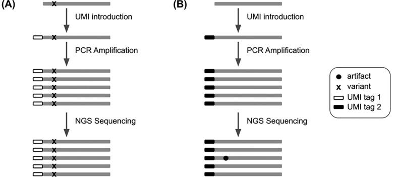
Detecting and calling out variants in the aligned reads is done through a variant calling analysis. Generally, variant calling tools can detect mutational events such as substitutions, insertions and deletions very efficiently. However, at very low variant allele frequencies (VAFs) (under 1%), it becomes very challenging for raw-read-based variant callers to accurately call variants. In fact, PCR amplification and the sequencing step can introduce errors in the final reads. These errors are called artifacts and occur at very low VAFs which can lead to the confusion between them and true low-frequency variants. Multiple studies [1], [2], [3], [4], [5] have shown the effectiveness of using Unique Molecular Identifiers as a way to filter out PCR and sequencing artifacts. UMIs are short arbitrary oligonucleotide sequences that are attached to DNA fragments by ligation before the PCR amplification. By definition, the UMI tags must be random sequences so each fragment can have a unique short oligonucleotide sequence attached to it, giving each fragment a unique sequence tag. During the amplification, the UMI tags are amplified with their respective fragments. After sequencing, each UMI tag can be figured out from the reads. The idea behind using UMI tags in NGS experiments to filter out artifacts is explained in Fig. 1. In fact, if a variant is a true mutation, it means that it must have been present on the initial DNA fragment so when we tag the DNA fragment with a UMI, we are also tagging the mutation. The fragments that result from the amplification of that mutated DNA fragment must all be tagged by the same UMI tag and carry the same mutation (Fig. 1A). On the other hand, if the variant is a sequencing error, it means that the initial DNA fragment did not have the mutation in the first place and that it appeared later in the sequencing step. Therefore, during the amplification step, all the fragments resulting from the amplification of that DNA fragment should theoretically be tagged with the same UMI and should not present the mutation. The mutation will be produced later on, in the sequencing step, affecting only some reads but not all of them, thus creating discrepancies in the same UMI group (Fig. 1B).

Fig. 1.

The difference between a true variant and an artifact from a UMI perspective. (A) A true variant is present on the DNA fragment so when the UMI tag 1 is added, it tags the fragment and the mutation as well. After amplification, all the fragments tagged with the UMI tag 1 carry the same mutation. (B) An artifact is not present on the DNA fragment but rather appears at the steps that follow the UMI introduction. That is why not all fragments with the same UMI tag 2 carry the same artifact.

With the growing number of variant calling tools, it has become hard to choose the right tool adapted to a certain experiment. Data simulation can play an important role for testing different tools on a dataset that we have control on, a control that we do not have on real biological data. At the moment, many short read simulators exist such as IntSIM [6] that can simulate somatic variants using HMM models trained on real sequencing genomes and SVSR [7] that is specifically designed to simulate datasets with structural variations and is compatible with multiple sequencing platforms. These tools are publicly available for researchers and allow them to test their algorithms on a simulated dataset in which variants are inserted at different frequencies and at different positions. The usage of the read simulators enable having a very accurate benchmarking of each variant calling tool ability. Surprisingly, no simulation software exists at the moment that let users generate reads with UMI tags. In this article, we present UMI-Gen, a UMI-based read simulator that can be used not only to test raw-read based variant callers but most importantly, UMI-based ones. UMI-Gen uses multiple real biological samples to estimate background error rate and base quality scores at each position. Then, it will introduce real variants in the final reads. To test our tool, we used 6 control samples and show exactly how our algorithm estimates the background error rate at each position. Then we give it a list of 15 variants at different positions and at different frequencies to introduce them in the final reads. Finally, we used 2 raw-read-based variant callers: SiNVICT[8] and OutLyzer [9] and two UMI-based variant callers: DeepSNVMiner [10] and UMI-VarCal [11] in order to compare the 4 tools performance and demonstrate that UMI-Gen correctly inserts the given variants at their respective positions and at the correct frequencies in a dataset that mimics perfectly what is seen in biological samples.

2. Materials and methods

2.1. Software input

UMI-Gen requires a minimum of three parameters at execution: a list of control BAM/SAM samples, the BED file with the coordinates of the targeted genomic regions and a reference genome FASTA file with BWA index files. In fact UMI-Gen is designed to work on targeted sequencing data only thus a BED file is always required. UMI-Gen can also accept a fourth optional file under the PILEUP format. In fact, when running UMI-Gen on control samples, a PILEUP file is automatically produced. This file contains the A, C, G and T average counts at each position for all the control samples. This file can be given to UMI-Gen at execution time and will allow the software to reload the pileup generated during the last analysis instead of regenerating it. This will allow the user to gain some significant time since the pileup generation is the most time-consuming step.

2.1.1. Control samples

Control samples are BAM/SAM files that are obtained by sequencing healthy individuals and normally should not contain any somatic variant. UMI-Gen can accept input files in BAM and SAM formats. A pileup is performed on each sample and a final average pileup is generated from the counts of all control samples.

2.1.2. Variant file

This file contains a list of the variants the user wishes to insert in the simulated reads. These are the only variants that should be reported in the variant callers VCF file during variant calling benchmarks. The variant file is a Comma Separated Values (CSV) file that contains 2 columns: the first column contains the variant ID with the HGVS nomenclature and the second column being the variant’s desired frequency. UMI-Gen will then go to each position and insert these variants in order to produce final reads.

2.2. Generating the final pileup

2.2.1. Pileup

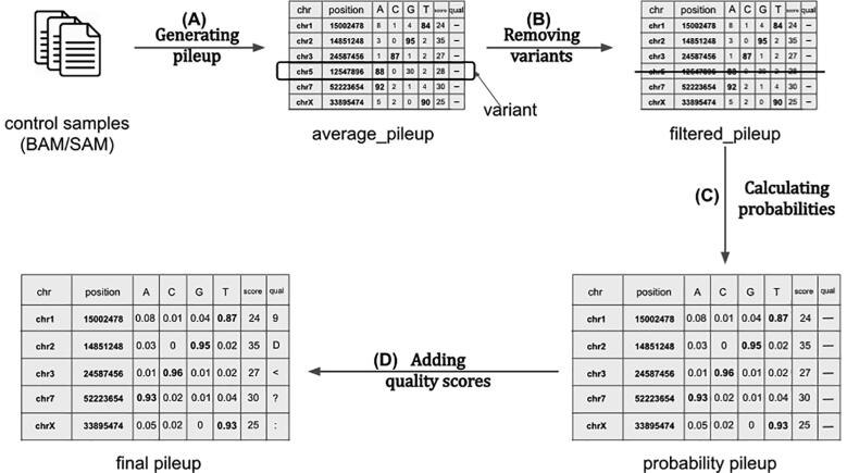
The first step of the workflow (Fig. 2) consists of generating the final pileup. For each control sample, our pileup algorithm will count the occurrences of each A, C, G and T. The counts will be stored for each position of the BED file as well as the average quality of the position and its depth. This is basically the same algorithm that is used by UMI-based variant caller UMI-VarCal that has been reintegrated in this tool for its high efficiency in treating reads with UMI tags. When all the pileups for all the control samples are ready, they will be merged in a final pileup that contains the average statistics (counts, depth and quality score) at each position based on the observations on all control samples (Fig. 2A). When the average pileup is complete and ready, it will be automatically dumped as a PILEUP file that contains all the calculated information on the set of control samples. If the user wishes to generate simulated data based on the same BED file and the same set of control samples, the dumped pileup can be used directly which allows the program to skip the pileup generation step and go directly to the variant calling step, saving the user much significant time.

Fig. 2.

Background error estimation workflow. (A) The first step runs over every position in all control samples and counts the total occurrences of every A, C, G and T. It also stores the average base quality score for each position. (B) The second step’s goal is to remove any suspected variant from the pileup as our objective is to estimate background error noise only. (C) In this step, the counts are converted to probabilities by dividing them by the depth for each position. (D) The final step consists of converting the base quality score of each position to the corresponding ASCII + 33 character.

2.2.2. Variant calling

Even though the control samples are theoretically variant-free, SNP and undetected mutations could still be present in the files. These potential variants must be removed so they would not be present in the final reads. To do so, we used the same variant calling method implemented in UMI-VarCal to call out potential variants and remove them from the pileup. This step will produce what we call a filtered pileup (Fig. 2B).

2.2.3. Background noise estimation

The background noise estimation step consists of calculating the frequency of observing an A/C/G/T at each position. Without the background errors, at each position the reference base should have a frequency of 1 while the remaining three bases should be at 0. The total of the four frequencies must be equal to 1. However, we know that artifacts exist in our control samples and these artifacts represent the background noise that we normally encounter in a normal NGS experiment. Since our aim is to simulate reads that are highly similar to those produced with real sequencing experiments, UMI-Gen calculates the real base frequencies from the control samples at each position. The frequencies will then be used as a probability matrix when producing the final reads. When this step is complete, a probability pileup is generated (Fig. 2C). Insertions and deletions are not considered during the background noise estimation and thus, are not present in the final pileup as their occurrence has a much lower rate (~1000 times lower) than that of substitutions) especially in second and third generation sequencers [12]. Therefore, we judge that their inclusion is not worth complicating the algorithm for.

2.2.4. Quality scores estimation

Our tool was developed on sequencing files produced by an Illumina sequencer. In the FASTQ files produced by Illumina sequencers, quality scores are encoded into a compact form, which uses only 1 byte per quality value [13], [14]. The full table of encoding is available in Table S1. UMI-Gen is therefore only compatible with sequencers that use the same encoding. UMI-Gen calculates the average quality score for each position based on the qualities in all control samples and then converts the quality score to the corresponding ASCII character to be inserted in the final FASTQ file. This is the final step of the pileup generation workflow and will produce the final pileup (Fig. 2D). Moreover, UMI-Gen also models the base quality scores per position in read on the control samples and introduces the estimation in the final reads. Based on all the reads in the control samples, our tool will calculate a median base quality score for each position in the reads to produce a quality per position matrix. This matrix is then used at the end to recalibrate the quality scores according to each base’s position in the read. For example, this allows UMI-Gen to mimic the loss of quality at the end of the reads when present.

2.3. Producing the reads

The main objective of UMI-Gen is to generate paired-end reads that mimic reads obtained from real life experiments. To do so, it starts exactly the way a real-life sequencing experiment starts: getting the DNA fragments. At the beginning, our tool will generate a number of initial sequences that only present the reference base at each position.

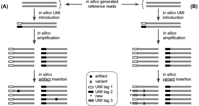
The user can explicitly specify the desired length for all the reads at execution. It should be noted that the algorithm will only create reads that will exactly align on the specified positions from the BED file so off-target amplification is not considered. Then, a UMI tag is attached to each initial sequence. Depending on the amplification factor and the desired depth chosen by the user, the algorithm will keep amplifying the initial sequences until the desired depth is reached at all positions. In fact, at this step, default values for the amplification factor and initial DNA fragments are automatically calculated in order to ensure optimal performance of the tool. We do so by analyzing the depth chosen by the user and the VAFs of the variants that he wishes to introduce. Using these numbers, we calculate the minimum number of initial DNA fragments needed for the true variant insertion. Even though this will ensure optimal performance, the user is free to change these parameters as long as they are mathematically allowed. Once we have the reference reads, the second step consists of adding the background noise (refer to Section 2.2.3) to these reads (Fig. 3A). Using the probability matrix calculated before, UMI-Gen modifies the reads at each position for them to match the calculated probabilities. These modifications are done without changing the reads’ UMI so they mimic PCR and sequencing artifacts: they are false positives and should not be called by variant callers. Finally, UMI-Gen parses the variant file provided by the user in order to insert true mutations in the final reads. The algorithm will go to each position, change the probability of the variant to the corresponding frequency from the variant file. In this step, since UMI-Gen is adding a true variant, the UMI tags of the modified reads are also modified in order to produce concordant UMI tags (Fig. 3B). A concordant UMI tag is a UMI whose all reads carry the exact same mutation. Also, since UMI-Gen generates paired-end data, when adding a mutation on one read, the variant is automatically added to its mate (since we only generate paired reads that always overlap).

Fig. 3.

The difference between adding a true variant and adding an artifact in generated reads. (A) Adding an artifact is relatively easy as all the tool has to do is to modify the base at the wanted position without touching the read’s UMI tag. (B) On the other hand, in order to add a true variant, the software must change the base at the wanted position on a set of reads. Then it will create a new UMI tag (UMI tag 3) and change the UMI tag of all the affected reads to UMI tag 3.

2.4. Software output

Once all variants are inserted, UMI-Gen will generate the two FASTQ files (R1 and R2). It will then call BWA [15] to do the alignment, a step that will produce a BAM file. SAMtools [16] is finally called to create the BAM’s index file and convert the BAM into SAM. All five files are generated in the desired output directory. In addition, UMI-Gen generates a binary PILEUP file that corresponds to the dumped average pileup. This file can be used to skip the pileup regeneration and load the pileup directly if the analysis was already done on the same control samples.

2.5. Implementation

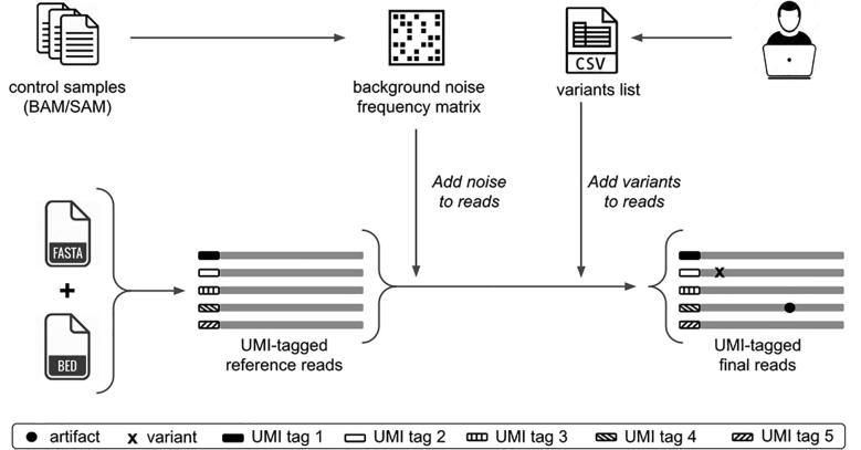
Launching UMI-Gen’s workflow (Fig. 4) is handled by a main Python script that controls many Python3 modules. In order to achieve better overall performance, Cython was used to compile all Python modules. UMI-Gen requires for the tools BWA and SAMtools to be installed on the PC/server: BWA is called for the alignment step and SAMtools for converting, sorting and indexing the generated BAM files. Our tool can be executed through a UNIX/Linux command line interface. In total, UMI-Gen can accept 20 parameters at execution. Managing these parameters allows the user to have full control over his simulated data. A list of all the parameters and thresholds is available in Table S2.

Fig. 4.

UMI-Gen’s workflow: Control samples are used to create a background noise frequency matrix and the user provides a CSV file with a list of the wanted variants. Using the FASTA and the BED files, UMI-Gen creates a first set of UMI-tagged reference reads. Artifacts are then inserted to mimic the sequencer’s background noise. Finally, the tool uses the list provided by the user to insert variants at their exact locations.

3. Results

3.1. Control samples

A targeted sequencing panel was designed at the Centre Henri Becquerel in Rouen (France) to search for specific mutations in the DNA of patients suffering from Diffuse Large B cell Lymphoma (DLBCL). This panel of 76,630 bases is designed to identify genomic abnormalities within a list of 36 genes that are most commonly impacted in this type of lymphoma. The panel was specifically designed for QIAseq chemistry allowing UMI introduction in the DNA fragments during the construction of the library. A list of the genes used in the panel and their corresponding number of targeted regions is provided in the supplementary Table S3. In order to test our tool’s ability to mimic and reproduce average sequencer background noise in the produced sample, we randomly selected 6 samples from a very large number of patients whose DNA were sequenced at the Centre Henri Becquerel. All six samples are liquid biopsies with circulating cell-free DNA that was checked to be adequate for sequencing. We preferred the use of liquid biopsies as these samples usually contain a high number of very low frequency variants and artifacts. Using such samples as control samples will produce simulated data with a relatively high number of artifacts. This will allow us to have an accurate estimate of the specificity of each tested variant caller.

Table 1 shows the exact counts of A, C, G, T for position 2,493,165 on chromosome 1 for each control sample. The fist control sample counts (0,11,10,874), the second sample has (0,1,7,843), the third one has (0,2,2,860), the fourth sample shows (1,6,9,965), the fifth one has (1,2,4,867) and the final one counts (3,2,2,880). As explained in Section 2.2.3, UMI-Gen will calculate an average count for each base and then estimate its probability. In our case and for this position, the obtained average count has 4 A, 24 C, 34 G and 5289 T with a total count of 5351 bases. To obtain the probabilities for this position on this chromosome, we simply divide each base count by the total count of the 4 bases, obtaining the final probability vector (0.0007, 0.0045, 0.0064, 0.9884). If, for example, we wanted to produce a BAM file with a depth of 3000x, this position would have 2 A, 14 C, 19 G and 2965 T. The probability matrix mentioned in Section 2.2.3 is basically the probability vectors of each position of the panel, merged together. In our test and in order to demonstrate our results, we simulated two artificial samples in which we added the calculated background error noise. The first sample or Sample 1 has an average depth of 1000× (+/− 15% at each position) and Sample 2 has an average depth of 10,000×. To make sure that the artifacts were correctly added to the reads, we used IGV (version 2.4.16) [17] to visualize the reads. Fig. 5 shows how the background error noise is properly and very accurately added at position 2,493,165 of chromosome 1 with the probabilities calculated from the 6 control samples above.

Table 1.

The A, C, G and T breakdown at position 2,493,165 of chromosome 1 for the six control samples.

Sample	A	C	G	T
Control 1	0	11	10	874
Control 2	0	1	7	843
Control 3	0	2	2	860
Control 4	0	6	9	965
Control 5	1	2	4	867
Control 6	3	2	2	880

Fig. 5.

The A, C, G and T breakdown at the position 2,493,165 of the chromosome 1 in the produced samples: Sample 1 with a depth of 1000× (A) and Sample 2 with the depth of 10,000× (B).

3.2. Simulated data validation

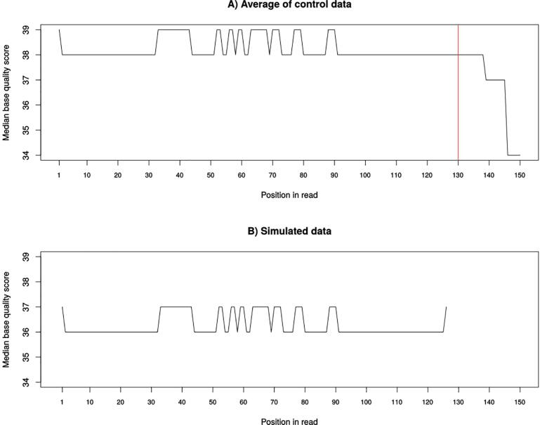
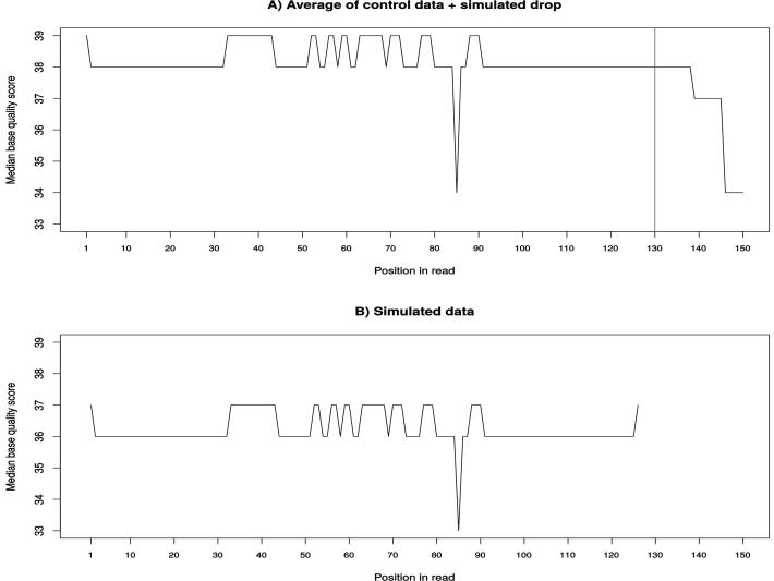
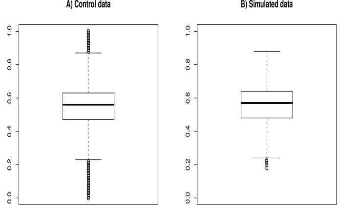
In order to validate our simulated dataset, we compared it to the control samples used to generate it. First, we compared the base quality scores distribution in the reads. Fig. 6A shows the variation of the median base quality scores with the position of base in the read for the control samples. We can clearly see that the median score is very high and very stable at the start and all along the read’s length (≥34). However, a first drop in quality is noted at position 138 and a second more considerable one at position 145. In our simulated data, we chose an average length for the reads of about 110 bp so the longest read had a length of 127. We can see, in Fig. 6B, how the algorithm perfectly recreates the stability of the scores all along the simulated reads. However, since the simulated reads did not have lengths >135 bp, we do not see that little drop at the end of the simulated reads. In fact, to be sure that our quality score estimation works correctly, we simulated a drop in quality at the position 85 and wanted to see if it will be inserted in the simulated reads. Fig. 7 shows how the simulated drop in quality (38 → 34) at position 85 was perfectly reproduced in the simulated data (36 → 33). Another parameter we wanted to verify is the %GC variation between the control and the simulated data. Fig. 8 clearly shows how the median %GC of reads in the control data (Fig. 8A – 56% GC) is nearly identical to that of the simulated reads (Fig. 8B – 57% GC).

Fig. 6.

The variation of the median base quality score with position in read in real samples (A) and in the simulated data (B).

Fig. 7.

The variation of the median base quality score with position in read in real samples (A) and in the simulated data (B). A simulated drop in quality was simulated in scenario A and its reproduction in the simulated dataset (B).

Fig 8.

The repartition of the %GC in reads in the real data (A) and in the simulated data (B).

3.3. Inserted variants

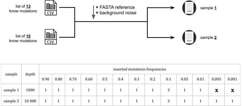
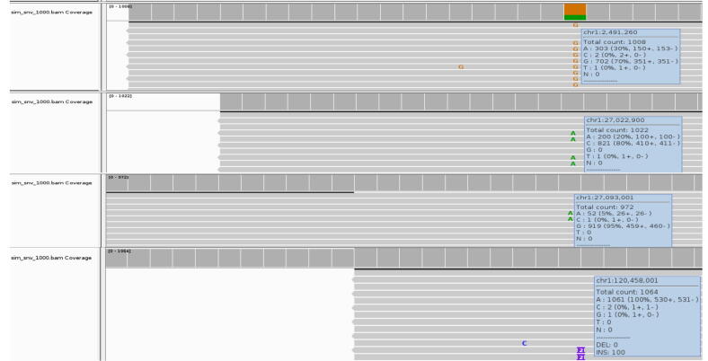
Two different lists of mutations were created to go along with each simulated sample. The first list contains 11 substitution variants with frequencies that go from 0.9 (90%) to 0.01 (1%), one deletion at 1% and one insertion at 1%. This list is used to produce the simulated Sample 1 with a depth of 1000x. The second list contains 13 substitution variants with frequencies that go from 0.9 (90%) to 0.001 (0.1%), one deletion at 1% and one insertion at 1%. This list is used to produce the simulated Sample 2 with a depth of 10,000x. Two very low frequency variants (frequency <1%) were added to the second list to test the variant insertion accuracy of UMI-Gen. In fact, very low frequency variants are the hardest to detect and should be systematically used to rigorously test any variant caller. In order to verify that the wanted variants were added at the exact locations with the correct frequencies, we used IGV to visualize the reads. Fig. 9 shows the variants added in both samples and Table 2 details the exact variants that we inserted at the specific locations. Next generation sequencers have difficulties with accurately detecting variants in long homopolymer regions. Some variant callers automatically filter out variants that occur in such regions and others do not. In order to avoid any bias, we chose each variant’s location carefully to make sure that it is not inserted in a homopolymer region. Fig. 10 demonstrates that our tool is capable of accurately adding variants in the final reads at the specified locations for both samples.

Figure 9.

Along with the reference genome FASTA file and the BED file, two different lists were used, one with 13 variants and the other with 15 variants to respectively produce the artificial samples Sample 1 and Sample 2.

Table 2.

Detailed list of the inserted mutations. In this test, all mutations are inserted on chromosome 1.

Position	Reference allele	Variant allele	Frequency	Sample
2,488,101	G	A	0.9	S1 & S2
2,489,200	C	A	0.8	S1 & S2
2,491,260	A	G	0.7	S1 & S2
2,493,201	T	A	0.6	S1 & S2
2,494,300	G	A	0.5	S1 & S2
23,885,600	C	A	0.4	S1 & S2
23,885,800	A	T	0.3	S1 & S2
27,022,900	C	A	0.2	S1 & S2
27,023,200	C	A	0.1	S1 & S2
27,093,001	G	A	0.05	S1 & S2
27,100,350	C	A	0.01	S1 & S2
27,106,500	G	A	0.005	S2 only
117,057,400	T	A	0.001	S2 only
120,458,000	C	CTA	0.1	S1 & S2
120,466,600	TGTC	T	0.1	S1 & S2

Figure 10.

The inserted mutations were correctly added to the reads with their exact locations at their corresponding frequencies. Here, we see four mutations: chr1:2491260A > G at 70%, chr1:27022900C > A at 20%, chr1:120458000C > CTA at 10% and chr1:27093001G > A at 5%.

3.4. Variant detection

We tested the ability of four different variant callers to correctly detect the true variants added in Section 3.3 and filter out sequencing errors/artifacts added in 3.1. We used SiNVICT and OutLyzer, two raw-read-based variant callers specifically developed to detect low frequency variants and two UMI-based variant callers (DeepSNVMiner and UMI-VarCal) with a very low frequency detection threshold and that analyze UMI tags in order to produce more accurate results. The four variant callers were tested on the two artificial samples: Sample 1 that contains 13 known variants and a depth of 1000× and Sample 2 that contains 15 known variants and a depth of 10,000×.

Both samples have a total of 76,630 sequenced positions which corresponds to the size of the sequencing panel. Table 3, Table 4 detail the results of each tool for Sample 1 and 2 respectively. The total number of positives corresponds to the number of variants found in the result VCF file. The total number of negatives is then calculated by subtracting total positives from the total number of positions (76,630). The four variant callers had comparable results between the two samples. Starting with SiNVICT, it detected 241 variants in Sample 1 and 463 in Sample 2 but with the same number of true positives. This corresponds to a sensitivity of 61.5%/53.4% which is relatively acceptable and a specificity of 99.7%/99.4% on Sample 1/2. Moving on to OutLyzer, the tool detected 109 variants in Sample 1 and three times more variants in Sample 2 (342). Unfortunately, this corresponded to one more true positive, the rest being only false positives. Outlyzer scored good sensitivities (>80%) and excellent specificities (99.9%/99.6%) on both samples.

Table 3.

Variant calling results on Sample 1. Four variant callers were tested: SiNVICT, OutLyzer, DeepSNVMiner and UMI-VarCal and for each tool, True Positives (TP), False Positives (FP), False Negatives (FN), sensitivity and specificity are reported.

Variant Caller	TP	FP	FN	Sensitivity (%)	Specificity (%)
SiNVICT	8	233	5	61.5	99.7
OutLyzer	11	98	2	84.6	99.9
DeepSNVMiner	12	37	1	92.3	99.95
UMI-VarCal	13	0	0	100	100

Table 4.

Variant calling results on Sample 2. Four variant callers were tested: SiNVICT, OutLyzer, DeepSNVMiner and UMI-VarCal and for each tool, True Positives (TP), False Positives (FP), False Negatives (FN), sensitivity and specificity are reported.

Variant Caller	TP	FP	FN	Sensitivity (%)	Specificity (%)
SiNVICT	8	455	7	53.4	99.4
OutLyzer	12	330	3	80	99.6
DeepSNVMiner	14	2	1	93.4	99.99
UMI-VarCal	15	0	0	100	100

Concerning DeepSNVMiner, the tool managed to detect all the inserted variants except the deletion in both samples. The tool scored very high scores on sensitivity (92.3%/93.4%) as well as specificity (99.95%/99.99%) for both datasets. Finally, UMI-VarCal was able to achieve a perfect score (100%] in terms of sensitivity and specificity on both samples detecting all the 13/15 variants in Sample 1/2 with no false positives for both configurations.

3.5. Performance

In order to evaluate UMI-Gen’s performance, we simulated four samples with increasing depths: 500, 1000, 5000 and 10,000. For each simulated sample, execution time and memory consumption were reported. The four samples were simulated using the same six control samples. The first time we run UMI-Gen, the pileup generation step is mandatory. The pileup generation step only depends on the control samples and takes about 1.5 min per sample. The quality estimation step following the pileup is also essential and takes on average 0.5 min per sample. However, these 2 steps generate files that can be given directly to the program at the execution. This means that for the other times the user wants to simulate data using the same control samples, the pileup file and the quality matrix file can be used directly allowing to save considerable time. Table 5 details the execution time numbers and the memory needed to generate each sample. Generating the FASTQ files takes only 1.57 min for the 500× sample and uses only 1 GB of RAM. On the other side, 16.58 min are needed for a sample of 10,000× and memory consumption goes up to 5.1 GB. All these tests were performed on a computer running Linux (Ubuntu 16.04) using only one core CPU running at 2.20 GHz and equipped with 16 GB of RAM. All measurements were done three times and the average was used for the comparison. After the FASTQ generation, BWA and SAMtools are called from within the tool to generate the corresponding BAM and SAM files.

Table 5.

Performance analysis of UMI-Gen: the variation of execution time and memory consumption with the simulated data’s depth.

Sample	Data Simulation (min)	FASTQ to BAM (s)	RAM Usage (GB)
500×	1.57	8	1.0
1000×	1.87	14	1.1
5000×	6.97	52	2.6
10,000×	16.58	99	5.1

4. Discussion

Tagging DNA fragments with UMI tags have proved itself as a very reliable method to significantly reduce – if not completely remove – the number of false positives upon variant calling. A huge number of variant callers are publicly available at the moment but unfortunately, only 4 of them are specifically developed to treat UMI tags in reads. For raw-read-based variant callers, a lot of artificial read simulators exist and can satisfy everyone’s needs. However, to our knowledge, no tool is publicly available to simulate artificial reads with UMI tags. Such a tool is very important as it allows developers to accurately test the specificity and the sensitivity of their variant callers on artificial reads in which real variants are known instead of testing them on biological samples whose mutational profile is completely or partially unknown.

Our main objective was to develop a UMI-based read simulator that is fast, accurate and reliable. UMI-Gen is able to estimate the background error noise of a given control dataset and then reproduce it accurately in the produced reads. Doing so, it allows to mimic the sequencer’s background noise of a real sequencing experiment. We also showed that our simulator is able to accurately insert variants if provided with a list of variants with exact locations and their corresponding frequencies and produce reads that mimic ones produced in real life experiments. In our tests, we were able to insert mutations as low as 0.1% but theoretically, we can go as low as we want provided that the depth of the produced sample is accordingly increased.

Moreover, in our variant caller comparison, SiNVICT did a decent job detecting the 8 of the added variants and went as low as 5%. Impressively, we judge the performance of OutLyzer as excellent as it detected 12 of the 15 variants (Sample 2) and showed a detection threshold of 0.5% which is very respectable. However, SiNVICT and OutLyzer being raw-read-based variant callers, UMI tags were not treated in the reads and therefore, both tools produced a high percentage of false positives. On the other hand, DeepSNVMiner results were near perfect as expected from a decent UMI-based variant caller detecting all variants except one in both scenarios with only a couple of false positives. Finally, UMI-VarCal was successfully able to treat UMI tags allowing it to filter out all false positives and only call out the 13 added variants in Sample 1 and all of the 15 in Sample 2. These results demonstrate how the UMI-based variant calling approach is much more efficient and accurate than raw-read-based ones allowing to detect variants with VAFs as low as 0.1% without sacrificing specificity. It also highlights the need to the development and usage of UMI-based read simulators in order to test these new algorithms.

5. Conclusion

Here, we present UMI-Gen: a standalone UMI-based read simulator for variant calling evaluation in paired-end sequencing NGS libraries. UMI-Gen produces sequencing files (FASTQ, BAM and SAM) for an artificial sample to be used for UMI-based variant calling testing purposes. By using a set of control DNA samples, our tool is capable of accurately mimicking the background error noise of the sequencer and adding it into the reads. After that, it can insert specific mutations at specific locations and at very precise frequencies that can go as low as 0.1% (and even lower). In our tests, all added artifacts were correctly inserted in the reads, causing a high number of false positives in the raw-read-based variant callers results. Also, all inserted true variants were visualized with a genome visualization tool (IGV) and were detected by at least one of the four variant calling tools we tested. Finally, we note that UMI-Gen’s filters and parameters (such as read length and UMI tag length) are customizable which gives the user total control over his produced samples. This level of customization allows the tool to be adequate for a high number of research applications.

Funding

This work was partly funded by the Université de Rouen Normandie and Vincent Sater is funded by a PhD fellowship from the Région Normandie.

CRediT authorship contribution statement

Vincent Sater: Conceptualization, Methodology, Software, Formal analysis, Data curation, Writing - original draft, Writing - review & editing, Visualization. Pierre-Julien Viailly: Conceptualization, Methodology, Resources, Data curation, Writing - original draft, Writing - review & editing, Visualization. Thierry Lecroq: Methodology, Writing - review & editing, Supervision, Project administration, Funding acquisition. Philippe Ruminy: Methodology, Supervision, Project administration. Caroline Bérard: Methodology, Formal analysis. Élise Prieur-Gaston: Conceptualization, Supervision. Fabrice Jardin: Resources, Supervision, Project administration.

Declaration of Competing Interest

The authors declare that they have no known competing financial interests or personal relationships that could have appeared to influence the work reported in this paper.

Appendix A. Supplementary data

The following are the Supplementary data to this article:

References

- 1.Schmitt M.W., Kennedy S.R., Salk J.J., Fox E.J., Hiatt J.B., Loeb L.A. Detection of ultra-rare mutations by next-generation sequencing. Proc Natl Acad Sci U S A. 2012;109:14508–14513. doi: 10.1073/pnas.1208715109. URL: https://www.ncbi.nlm.nih.gov/pmc/articles/PMC3437896/ [DOI] [PMC free article] [PubMed] [Google Scholar]
- 2.Kukita Y., Matoba R., Uchida J., Hamakawa T., Doki Y., Imamura F. High-fidelity target sequencing of individual molecules identified using barcode sequences: de novo detection and absolute quantitation of mutations in plasma cell-free DNA from cancer patients. DNA Res. 2015;22:269–277. doi: 10.1093/dnares/dsv010. URL: https://www.ncbi.nlm.nih.gov/pmc/articles/PMC4535617/ [DOI] [PMC free article] [PubMed] [Google Scholar]
- 3.Newman A.M., Lovejoy A.F., Klass D.M., Kurtz D.M., Chabon J.J., Scherer F. Integrated digital error suppression for improved detection of circulating tumor DNA. Nat Biotechnol. 2016;34:547–555. doi: 10.1038/nbt.3520. URL: https://www.ncbi.nlm.nih.gov/pmc/articles/PMC4907374/ [DOI] [PMC free article] [PubMed] [Google Scholar]
- 4.Young A.L., Challen G.A., Birmann B.M., Druley T.E. Clonal haematopoiesis harbouring AML-associated mutations is ubiquitous in healthy adults. Nat Commun. 2016;7 doi: 10.1038/ncomms12484. URL: https://www.ncbi.nlm.nih.gov/pmc/articles/PMC4996934/ [DOI] [PMC free article] [PubMed] [Google Scholar]
- 5.Bar D.Z., Arlt M.F., Brazier J.F., Norris W.E., Campbell S.E., Chines P. A novel somatic mutation achieves partial rescue in a child with Hutchinson-Gilford progeria syndrome. J Med Genet. 2017;54:212–216. doi: 10.1136/jmedgenet-2016-104295. URL: https://www.ncbi.nlm.nih.gov/pmc/articles/PMC5384422/ [DOI] [PMC free article] [PubMed] [Google Scholar]
- 6.Yuan X., Zhang J., Yang L. IntSIM: An integrated simulator of next-generation sequencing data. IEEE Trans Biomed Eng. 2017;64:441–451. doi: 10.1109/TBME.2016.2560939. [DOI] [PubMed] [Google Scholar]
- 7.Yuan X., Gao M., Bai J., Duan J. SVSR: A program to simulate structural variations and generate sequencing reads for multiple platforms. IEEE/ACM Trans Comput Biol Bioinf. 2020;17:1082–1091. doi: 10.1109/TCBB.2018.2876527. [DOI] [PubMed] [Google Scholar]
- 8.Kockan C., Hach F., Sarrafi I., Bell R.H., McConeghy B., Beja K. SiNVICT: ultra-sensitive detection of single nucleotide variants and indels in circulating tumour DNA. Bioinformatics. 2017;33:26–34. doi: 10.1093/bioinformatics/btw536. [DOI] [PubMed] [Google Scholar]
- 9.Muller E., Goardon N., Brault B., Rousselin A., Paimparay G., Legros A. OutLyzer: software for extracting low-allele-frequency tumor mutations from sequencing background noise in clinical practice. Oncotarget. 2016;7:79485–79493. doi: 10.18632/oncotarget.13103. URL: https://www.ncbi.nlm.nih.gov/pmc/articles/PMC5346729/ [DOI] [PMC free article] [PubMed] [Google Scholar]
- 10.Andrews T.D., Jeelall Y., Talaulikar D., Goodnow C.C., Field M.A. DeepSNVMiner: a sequence analysis tool to detect emergent, rare mutations in subsets of cell populations. PeerJ. 2016;4 doi: 10.7717/peerj.2074. URL: https://www.ncbi.nlm.nih.gov/pmc/articles/PMC4888318/ [DOI] [PMC free article] [PubMed] [Google Scholar]
- 11.Sater V., Viailly P.-J., Lecroq T., Prieur-Gaston E., Bohers E., Viennot M. UMI-VarCal: a new UMI-based variant caller that efficiently improves low-frequency variant detection in paired-end sequencing NGS libraries. Bioinformatics (Oxford, England) 2020 doi: 10.1093/bioinformatics/btaa053. [DOI] [PubMed] [Google Scholar]
- 12.Schirmer M., Damore R., Ijaz U.Z., Hall N., Quince C. Illumina error profiles: resolving fine-scale variation in metagenomic sequencing data. BMC Bioinf. 2016;17 doi: 10.1186/s12859-016-0976-y. URL: https://www.ncbi.nlm.nih.gov/pmc/articles/PMC4787001/ [DOI] [PMC free article] [PubMed] [Google Scholar]
- 13.Ewing B., Green P. Base-calling of automated sequencer traces using Phred. II. Error probabilities. Genome Res. 1998;8:186–194. doi: 10.1101/gr.8.3.186. URL: http://genome.cshlp.org/content/8/3/186. [DOI] [PubMed] [Google Scholar]
- 14.Ewing B., Hillier L., Wendl M.C., Green P. Base-calling of automated sequencer traces using Phred. I. Accuracy assessment. Genome Res. 1998;8:175–185. doi: 10.1101/gr.8.3.175. URL: http://genome.cshlp.org/content/8/3/175. [DOI] [PubMed] [Google Scholar]
- 15.Li H., Durbin R. Fast and accurate short read alignment with burrows-wheeler transform. Bioinformatics. 2009;25:1754–1760. doi: 10.1093/bioinformatics/btp324. URL: https://www.ncbi.nlm.nih.gov/pmc/articles/PMC2705234/ [DOI] [PMC free article] [PubMed] [Google Scholar]
- 16.Li H., Handsaker B., Wysoker A., Fennell T., Ruan J., Homer N. The sequence alignment/map format and SAMtools. Bioinformatics. 2009;25:2078–2079. doi: 10.1093/bioinformatics/btp352. URL: https://www.ncbi.nlm.nih.gov/pmc/articles/PMC2723002/ [DOI] [PMC free article] [PubMed] [Google Scholar]
- 17.Robinson J.T., Thorvaldsdóttir H., Winckler W., Guttman M., Lander E.S., Getz G., Mesirov J.P. Integrative genomics viewer. Nat Biotechnol. 2011;29:24–26. doi: 10.1038/nbt.1754. URL: https://www.ncbi.nlm.nih.gov/pmc/articles/PMC3346182/ [DOI] [PMC free article] [PubMed] [Google Scholar]
Associated Data
This section collects any data citations, data availability statements, or supplementary materials included in this article.