Abstract
Maize (Zea mays L.) is the essential staple in sub-Saharan Africa (SSA) and Tanzania in particular; the crop accounts for over 30% of the food production, 20% of the agricultural gross domestic product (GDP) and over 75% of the cereal consumption. Maize is grown under a higher risk of failure due to the over-dependence rain-fed farming system resulting in low income and food insecurity among maize-based farmers. However, many practices, including conservation agriculture, soil and water conservation, resilient crop varieties, and soil fertility management, are suggested to increase cereal productivity in Tanzania. Improving planting density, and the use of fertilizers are the immediate options recommended by Tanzania's government. In this paper, we evaluate the economic feasibility of the improved planting density (optimized plant population) and N-fertilizer crop management practices on maize net returns in semi-arid and sub-humid agro-ecological zones in the Wami River sub-Basin, Tanzania. We introduce a bio-economic simulation model using Monte Carlo simulation procedures to evaluate the economic viability of risky crop management practices so that the decision-maker can make better management decisions. The study utilizes maize yield data sets from two biophysical cropping system models, namely the APSIM and DSSAT. A total of 83 plots for the semi-arid and 85 plots for the sub-humid agro-ecological zones consisted of this analysis. The crop management practices under study comprise the application of 40 kg N-fertilizer/ha and plant population of 3.3 plants/m2. The study finds that the use of improved plant population had the lowest annual net return with fertilizer application fetching the highest return. The two crop models demonstrated a zero probability of negative net returns for farms using fertilizer rates of 40 kg N/ha except for DSSAT, which observed a small probability (0.4%) in the sub-humid area. The optimized plant population presented 16.4% to 26.6% probability of negatives net returns for semi-arid and 14.6% to 30.2% probability of negative net returns for sub-humid zones. The results suggest that the application of fertilizer practices reduces the risks associated with the mean returns, but increasing the plant population has a high probability of economic failure, particularly in the sub-humid zone. Maize sub-sector in Tanzania is projected to continue experiencing a significant decrease in yields and net returns, but there is a high chance that it will be better-off if proper alternatives are employed. Similar studies are needed to explore the potential of interventions highlighted in the ACRP for better decision-making.
Keywords: Bio-economic simulation, APSIM, DSSAT, Crop-management practices, Risk, Maize, Tanzania
1. Introduction
Maize (Zea mays L.) is a major staple food crop in sub-Saharan Africa (SSA) grown in diverse agro-ecological zones and farming systems. The crop is predominantly consumed by people with varying food preferences and socioeconomic backgrounds. Maize accounts for almost half of the calories and protein consumed in eastern and southern Africa (Macauley and Ramadjita, 2015). In Tanzania, maize accounts for around 30% of overall food production, over 75% of cereal consumption and between 20 and 30% of the total agricultural gross domestic product (GDP) with 70% of the population eat maize as their staple food (URT, 2014; Wilson and Lewis, 2015). Tanzania is the dominant producer for maize in eastern and central Africa (Waithaka et al., 2013).
However, like many other cereal sub-sectors in Tanzania, the maize sub-sector is grown under a higher risk of failure due to high dependence on a rain-fed farming system and low ability to adapt to climatic variability (URT, 2014). Mostly, the maize sub-sector is sensitive to even a small change in temperature and precipitation in Tanzania and SSA in general (Waithaka et al., 2013; URT, 2014; Kahimba et al., 2015). Hence, given the importance of maize in SSA where the vast majority of the world's poor people are located, exploring agronomic and management practices that will help the sector progress has recently attracted attention from several governments (Waithaka et al., 2013; Kahimba et al., 2015; Msongaleli et al., 2015; Richardson and Bizimana, 2017).
To address the challenges hindering agricultural production in Tanzania, the government has introduced policies, strategies, and guidelines to stimulate the sector. These include the Tanzania National Adaptation Program of Action (NAPA) formulated in 2007 (URT, 2007), Climate-Smart Agricultural Guideline (URT, 2017), and Agriculture Climate Resilience Plan (ACRP) 2014–2019 (URT, 2014). Others are National Agricultural Policy (URT, 2013) and the Agricultural Sector Development Programme phase two (ASDP-II), to mention a few (URT, 2016). These policies and strategies listed several potential agronomic and technology practices that would help integrate resilience in agricultural policy decisions, influence the planning process, and implement investment on the ground. The ACRP pinpointed several intervention practices that sustainably increases productivity, resilience, and enhances the achievement of national food security and reduces poverty. These practices include conservation agriculture (e.g., crop rotation, contour cropping), soil and water conservation (mulching, terracing), resilient crop varieties (drought/heat-tolerant varieties, pest & disease-resistant varieties), cropland management (cover crop, reduced tillage), soil fertility management (fertilizers, mulching) and agro-forestry (crop tree planting, tree nurseries).
Of all the practices identified by the ACRP 2014–2019, improving planting density and the use of fertilizers were the immediate options recommended because of their expected ease in realizing yield benefits, particularly in high rainfall areas or seasons (URT, 2007; URT, 2014; Msongaleli et al., 2015). The interventions are proposed to be implemented either at the country level or in the selected agro-ecological zones like the alluvial plains, northern highlands, plateau, semi-arid lands, southwestern highlands, southern highlands, and western highlands. Although the government suggested several options to be implemented in different agro-ecological zones, their economic feasibility should be known to the majority so they can make better decisions. Lack of enough information on the proposed alternative management practices' economic viability may hinder the adoption and proper use of the technologies. Feder et al. (1985) argued that adoption at the individual farmers' level is defined as the degree of use of new technology in the long-run equilibrium when the farmer has full information about the new technology and its potential. Based on Feder's argument, the most critical problem on the adoption of a technology/intervention is the one related to the information asymmetric.
On the other hand, detailed assessment studies that link data from biophysical and economic models are required to provide relevant information on the probable benefits of the proposed agronomic practices for better decision-making (Thompson et al., 2010; White et al., 2011; Kahimba et al., 2015; Rosenzweig et al., 2015). The use of multiple-models in assessment studies has shown to enhance the quantification of uncertainties and reliabilities as different models differ in structure and parameterization (Rötter et al., 2011; Msongaleli et al., 2015). With this regard, the Agricultural Model Inter-comparison and Improvement Project (AgMIP) highlights procedures to utilize multiple models (Rosenzweig et al., 2015). The AgMIP realizes on the importance of integrating biophysical and socioeconomic models to improve decision-making in agricultural production systems.
The objective of the present work is to demonstrate the benefits of using Monte Carlo simulation techniques to examine the economic viability of two risky alternatives, namely N-fertilizer application and plant population adjustment. The study develops a practical framework that links data from biophysical process-based models to build a Monte Carlo bio-economic simulation model, used to estimate the distribution of economic returns for alternative management strategies. Two biophysical models, namely the Agricultural Production Systems sIMulator (APSIM) and Decision Support System for Agro-technology Transfer (DSSAT) cropping systems models, were used to develop a bio-economic simulation model. The two biophysical models are recommended for integrated assessment in SSA to improve decision-making for farm managers and policy-makers (Rosenzweig et al., 2015). A bio-economic simulation model using a Monte Carlo simulation procedure was developed to link the baseline and alternative data from the two biophysical models. A Monte Carlo simulation approach to assess the economic feasibility of management practices in the agricultural sector has been used by Richardson et al. (2008), Palma et al. (2011), Rezende and Richardson (2015), Richardson and Bizimana (2017) and more recently by Bizimana and Richardson (2019).
2. Materials and methods
This study is part of modeling activities under AgMIP protocols (Rosenzweig et al., 2015) conducted from 2015 to 2017 with improved computing tools for enhanced regional integrated assessment studies in developing countries, including SSA (see Version 6 of the AgMIP handbook of methods and procedures at www.agmip.org). The AgMIP protocols recommend implementing two crop models (DSSAT and ASPIM) and at least one socioeconomic model.
2.1. Study area
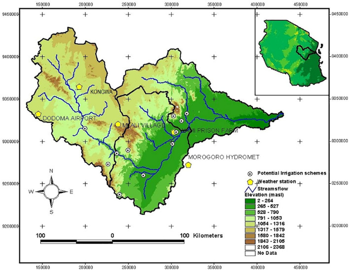
The maize plots used in the present study are located in the Wami River sub-Basin of Tanzania. The Wami River sub-Basin lies between 5°–7°S and 36°–39°E, where it extends from the semi-arid in Dodoma region to the humid inland swamps in Morogoro region, to the Saadani village at the coast of Indian Ocean (Fig. 1 ). It covers an area of approximately 43,000 km2, with altitude ranging from 0 m at the coast to 2260 m in Ukaguru Mountains.
Fig. 1.
Study site: Wami River sub-basin, Tanzania.
Wami River sub-Basin is characterized by crop production, livestock keeping with numerous off-farm activities. The study area is dominated by smallholder farms, growing an array of crops including maize, sorghum, rice, legumes, cassava, groundnuts, millet, and beans. Maize is the staple food crop in the study area. The area's onset of rainfall usually occurs in mid-September. The rainy season extends until April in the sub-humid part and early-mid December to April in a semi-arid region. The availability of weather stations in the study area (Kongwa, Dodoma airport, Malali, Wami prison, and Morogoro) provide useful weather data needed by the two crop models (Fig. 3.1).
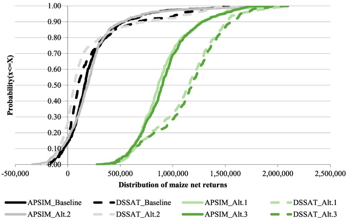
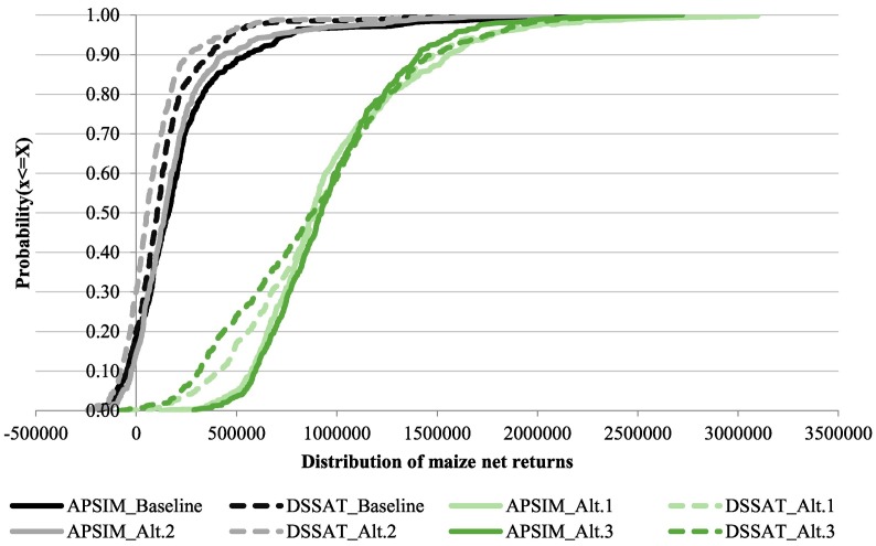
Fig. 3.
CDF of annual net return in semi-arid as for APSIM and DSSAT cropping models.
2.2. Data and modeling framework
The bio-economic model is a Monte Carlo simulation approach to simulate the key output variables (KOVs), including revenues (yield x price) and net cash returns, using yield and price risk associated with different management practices. The model uses maize yield data (with and without management practices) obtained from work done by Tumbo et al. (2020) in which two process-based crop models were used. The two models were the Agricultural Production Systems sIMulator (APSIM) and the Decision Support System for Agrotechnology Transfer (DSSAT). These models employed maize production data from the second wave of the Tanzania National Panel Survey (TNPS) (NBS – National Bureau of Statistics, 2012). A total of 168 maize plots within the Wami River sub-Basin were sorted (83 plots for the semi-arid part and 85 plots for the sub-humid part). The TNPS also provided data on production costs, the area planted, and all inputs used for maize production. The average area for maize plots size was 1.26 ha and 1.76 ha for semi-arid and sub-humid, respectively. Table 1 displays the distribution of the area planted to maize used in this study. However, the information on maize prices was obtained from regional agricultural offices (marketing unit) within the basin to have all the necessary information to model the key output variables (KOVs). The bio-economic model incorporated the risk of maize production in the Wami River sub-Basin by using probability distributions to simulate random values for yields, prices, and costs.
Table 1.
Distribution of maize plots (ha) per agro-ecological zone in Wami River sub-basin.
| Zone | Average | Minimum | Maximum | Total area |
|---|---|---|---|---|
| Semi-arid | 1.26 | 0.5 | 2.8 | 97.4 |
| Sub-humid | 1.76 | 0.8 | 3.80 | 158.3 |
Source: TNPS.
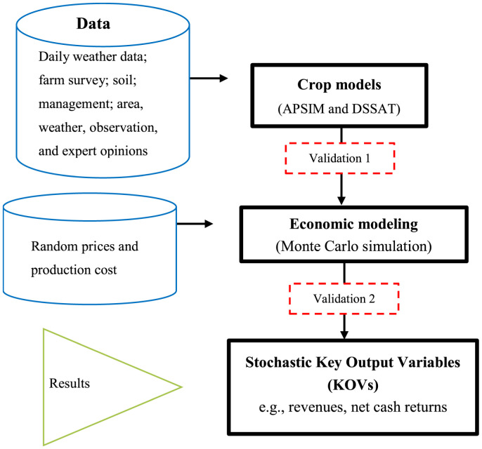
Fig. 2 presents a diagram of the bio-economic model. The diagram shows that the simulated yield from the two biophysical models was first validated (Validation 1) by comparing the simulated yield probability distribution functions (PDFs) to the biophysical baseline observed yield distributions (Appendix A). With the similarities in the PDFs, the yield data from the two process-based models were used to develop a Monte Carlo bio-economic model, as explained in the sub-2.4, 2.5, 2.6, 2.7. Before applying a Monte Carlo bio-economic simulation model, the data were validated again (Validation 2) to ensure that the random variables are simulated correctly and demonstrate the appropriate properties of the two crop models (see section 2.5). After the second validation, the last activity in the model was to estimate the KOVs, discuss them, and conclude. The bio-economic simulation model was developed using the Simetar add-in [www.simetar.com] in Microsoft Excel following the protocols developed by Richardson et al., 2000, Richardson et al., 2008.
Fig. 2.
Bio-economic simulation model.
2.3. Overview of APSIM and DSSAT cropping system models
APSIM) is a modeling environment software tool that enables sub-models to be linked to simulate agricultural systems. APSIM uses various tools and component modules to dynamically simulate cropping systems in the semi-arid tropics (McCown et al., 1996; Wolday and Hruy, 2015). The model simulates the mechanistic growth of crops, soil processes, and a range of options considering the cropping system perspective (McCown et al., 1996). APSIM was designed as a farming systems simulator to combine accurate yield estimation in response to management with the prediction of the long-term consequences for alternative farming practices (Keating et al., 2003). Required inputs for APSIM include: weather, soil, crop data, and management options (Ahmed and Hassan, 2011).
DSSAT is a software application program that comprises crop simulation models for over 42 crops as well as tools to facilitate effective use of the models (Hoogenboom et al., 2017). The crop simulation models simulate growth, development, and yield as a function of the soil-plant-atmosphere dynamics under specified management practices over time (Jones et al., 2001, Jones et al., 2003). DSSAT includes database management programs for soil, weather, crop management, and experimental data, utilities, and application programs. DSSAT and APSIM crop models allow users to simulate options for alternative crop management scenarios to assess yield risks (Ahmed and Hassan, 2011).
In this study, APSIM and DSSAT provided the processed maize yield with-and without the recommended management practices. Different biophysical parameters like soil type, management practices (cultivars, planting dates, fertilizer application, and plant population) and climate/weather available within the basin were included in the model (Tumbo et al., 2020). Increasing soil fertility and planting density adjustment were two alternative practices considered. For each farm, a 40 Kg N/ha was applied for soil fertility and 33,000 plants/ha (3.3 plants/m2) and simulated by APSIM and DSSAT cropping systems, as detailed by Tumbo et al. (2020).
2.4. Overview of the proposed interventions
Increasing soil fertility through fertilizer application and improving planting density were two interventions considered in this study. The two options are highlighted in the ACRP 2014–2019 as the immediate interventions for improving maize and other cereals productivity. Historically, Tanzania has had a low level of fertilizer application, among the lowest in the world. In 2010, this averaged only about 9 kg/ha/year, and it reached 12.6 kg/ha/year in 2016 as a result of the input subsidy (Wilson and Lewis, 2015; The World Bank, 2020). Although the current data shows an increasing trend for fertilizer consumption per unit area, there is a possibility of dropping because of the COVID-19 impacts on fertilizer prices, as many of the fertilizers are imported. Maize production consumes over 56% of all the fertilizers used. According to IFDC (2012), the Wami-Ruvu basin is within regions where the proportion of farmers using fertilizers is below 5%. A current study by Tumbo et al. (2020), highlighted that the percentage of farms using inorganic fertilizers in Wami Sub-basin is very low, ranging between 3% to 13%. The small fertilizer application is because over 80% of the maize producers are dominated by smallholder farmers who sometimes minimize their production cost by choosing not to use the recommended fertilizers (Wilson and Lewis, 2015).
Most of the farms in the study did not use fertilizers. Therefore, DSSAT and APSIM crop models were used to identify the optimum fertilizer rate and the planting density suitable for the Wami River sub-Basin under current climate and current farm management practices. The procedures for the selection of fertilizer rates and plant populations are well documented by Rao et al. (2015) and Tumbo et al., 2015, Tumbo et al., 2020. The fertilizer rate of 40 kg N/ha was therefore selected for use within the Wami River sub-Basin. The increased plant population to 33,000 plant/ha (3.3 plants/m2) was chosen which is a significant increase from the current rates of 18,000–22,000 plants/ha (20,000 plants/ha on average).
2.5. Bio-economic modeling framework
The development of the bio-economic simulation model involved five stages. The first stage was to validate the original or observed data from the survey and baseline data from the two biophysical, process-based crop models. The details of the baseline data have been reported by Tumbo et al. (2020). The output from the two models was used to develop a bio-economic simulation model. Four scenarios under study are summarized below:
-
•
BASELINE: current agricultural farming system;
-
•
ALT.1: baseline plus fertilizer application of 40 kg N/ha for all the plots.
-
•
ALT.2: baseline plus plant population of 33,000 plants/ha (3.3 plants/m2).
-
•
ALT.3: baseline plus (ALT.1 + ALT.2).
The above-described scenarios make a total of 16 simulations for the bio-economic model. That is 1 scenario for two models for two agro-ecological zones (BASELINE = 2 × 2; ALT.1 = 2 × 2; ALT.2 = 2 × 2 and ALT.3 = 2 × 2). Since we have multiple scenarios, the multivariate empirical (MVE) distribution described by Richardson et al. (2000) was used to account for all 16 scenarios. MVE distributions are defined by the fractional deviations from the mean (Sijω) and cumulative probabilities (F(Sijω)) where i indicates maize yield for each scenario, for crop model j per zone ω to estimate the probability distributions. We programmed the economic model in Microsoft Excel using the Simetar add-in, following a detailed Monte Carlo simulation modeling procedure described by Richardson et al. (2000).
2.6. Stochastic yields
To simulate the stochastic component of the model for analyzing risky alternatives, a vector of uniform standard deviates (USDs) was computed first. USD is a probability distribution included in Simetar to produce a uniform standard deviate on the 0–1 scale and is simulated with a function = UNIFORM(). It is used to simulate several random variables for all probability distributions via the inverse transformation method of generating random variables (Richardson et al., 2008). The resulting vector is used to simulate random yields for each scenario analyzed for all cropping system models.
| (1) |
Where = random mean yield/ha,
i = scenarios (BASELINE, ALT.1, ALT.2 AND ALT.3),
j = crop model (APSIM and DSSAT),
ω = agro-ecological zones (semi-arid and sub-humid).
Sijω = sorted deviations from mean (percentage deviations from the mean).
F(Sijω) = the frequency distribution for the fractional deviates from the mean.
MVEMP = Simetar function used to simulate a MVE defined by Sijω and F(Sijω) and the correlation matrix for the random deviates indicated as CUSDs.
Each scenario in Eq. 1 was simulated for 500 iterations to provide an adequate sample of the yields to simulate economic KOVs to estimate their probability distributions and relative variabilities. The simulated yields were validated to check for model completeness, accuracy, and simulation ability. PDF charts for bio-economic simulated vs. process-based data for all the agro-ecological zones data were developed for this purpose. A detailed procedure for how the results of bio-economic simulation results were validated is provided in Appendix B. Due to limited space, only the validation PDFs for semi-arid areas are presented in the Appendix, but the procedures of the bio-economic simulation model to simulate the process-based data sets were met for all the agro-ecological zones.
2.7. Stochastic prices and receipts
Maize price within the basin was simulated using a GRKS distribution. The GRKS distribution was developed by Gray, Richardson, Klose, and Schumann to simulate subjective probability distributions based on minimum, mid-point, and maximum input data (Richardson et al., 2008). Simetar simulates it with the = GRKS(min, mid-point, max) function. The output from GRKS is a stochastic price denoted in this study by (). The stochastic prices were combined with the yield for each scenario in Eq.1 to simulate the stochastic receipts (). Table 2 provides the distribution of maize prices used to parameterize the GRKS distribution (Eq. 2). The equation for the stochastic revenue for each scenario was given by Eq. 3.
| (2) |
| (3) |
Table 2.
Annual price distribution for maize grains in the Wami River sub-basin.
| Semi-arid (TZS/t) | Sub-humid (TZS/t) | |
|---|---|---|
| Minimum | 445,556 | 356,725 |
| Average | 555,830 | 542,100 |
| Maximum | 666,811 | 694,082 |
Source: Regional Agricultural Office in Dodoma and Morogoro.
2.8. Production costs and net returns
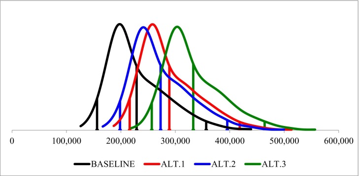
The production cost for the baseline scenario is composed of field preparation costs, planting costs, farm management costs, harvesting, and transportation. Table C1 in Appendix C summarizes the typical production cost incurred by farmers in Wami River sub-Basin. The cost of the proposed interventions was included in the model. This involved addition of fertilizer and increased seeding rates, both of which imply increases in production cost. Thus, the total variable cost of production is expected to increase (Rao et al., 2015). We calculated the additional cost for the farmer to purchase the 40 kg of nitrogen fertilizer and the additional cost of buying extra kilograms of maize seeds to make a required of ≥33,000 plants/ha. With consideration of expert opinions, it was argued that the current average plant population in the Wami River sub-Basin is between 18,000 and 22,000 plants/ha (20,000 plants/ha on average), which is equivalent to 18–22 kg/ha. Therefore, 7–10 kg is needed to make the plant population per ha ≥ 33,000.
With this regard, it was agreed that the cost of 40 kg N ranges from TZS 55,000 to TZS 65,000 (TZS 60,000 on average), including transport and labor charges. One kilogram of maize seeds ranges from TZS 4000 to TZS 6000, hence farmers are likely to incur an additional cost of between TZS 28,000 to TZS 60,000 to purchase extra seeds. Fig. C1 in Appendix C displays the distribution of production cost per ha per scenario used in the bio-economic model. Again, the GRKS distribution was used to simulate the stochastic production cost () for the baseline and alternatives. It was also observed that the distribution of production cost per ha for the baseline scenario was the same for sub-humid and semi-arid areas in the basin with the same distribution for the risky alternatives (Table 3 ). The costs for each scenario in Table 3 were, therefore, simulated in Simetar using the function in Eq. 4. Net returns for each scenario (Eq. 5) were calculated as the total receipt minus total cost.
| (4) |
| (5) |
Table 3.
Distribution of costs for the baseline and the alternative scenario within the Wami River sub-basin (TZS/ha).
| BASELINE | ALT.1 | ALT.2 | ALT.3 | |
|---|---|---|---|---|
| Minimum | 155,000 | 215,000 | 200,000 | 260,000 |
| Average | 210,000 | 270,000 | 254,000 | 314,000 |
| Maximum | 360,000 | 420,000 | 404,000 | 464,000 |
Source: TNPS.
Where: Minimum is the minimum production cost (TZS/ha) value for the distribution,
Maximum is the maximum production costs (TZS/ha) value for the distribution,
Average is the average production cost (TZS/ha) value for the distribution
The bio-economic simulation model results were presented using tables as well as the Cumulative Distribution Functions (CDF) and the Probability Distribution Functions (PDF). The PDF and the CDF were drawn to estimate the distribution of economic returns for scenarios so decision-makers can make better decisions. The results of the model were also presented using the Stoplight Chart. The Stoplight Chart is a function in Simetar used to develop ranking probabilities. It summarizes the probabilities that the KOV(i.e., net returns) for scenarios/alternatives will be less than the lower target and the probability the KOV will exceed a maximum target (Richardson et al., 2008; Bizimana and Richardson, 2019; Kadigi et al., 2020). We set the minimum net returns target to be TZS 0 and the maximum target to be the average maize returns per ha, which is around TZS 500,000. The Stoplight chart estimated the probabilities of net profits falling below zero (being negative), exceeding TZS 500,000, and the probabilities of falling between the two targets.
3. Results and discussion
3.1. Relative risks for baseline and alternative scenarios on maize yield in the Wami River sub-basin
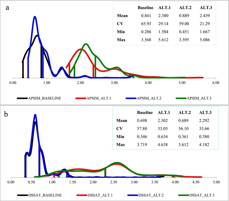
The first thing performed by this study is the evaluation of the relative variability about the mean yield for each risk alternative analyzed. Yield data from the two process-based crop models (APSIM and DSSAT) were simulated using a Monte Carlo simulation procedure for 500 iterations to capture the relative risks associated with maize yield for each scenario (Table 4 ). The table provides the mean, standard deviation (SD), coefficient of variation (CV), minimum and maximum statistics for each alternative. The CV measures the relative risk associated with the mean yield per scenario for each agro-ecological zone in the basin. Both APSIM and DSSAT reported the highest CVs for the BASELINE scenario and ALT.2 with relatively small CVs for ALT.1 and ALT.3 in both agro-ecological zones. BASELINE in semi-arid has a CV equal to 63.9% and 74.2% for APSIM and DSSAT; and in the sub-humid region the BASELINE has a CV equal to 65.9% and 57.9% for the two models, respectively. Of all the scenarios, ALT.2 had CV values closer to BASELINE for both APSIM and DSSAT models with ALT.1 and ALT.3 having the smallest CVs of between 18.4% and 29.1% for APSIM and 20.5% and 33.7% for DSSAT. The simulation results indicate that the BASELINE and ALT.2 have the highest relative risk.
Table 4.
Summary statistics for the stochastic distribution of maize yield of the bio-economic simulation model.
| APSIM |
DSSAT |
|||||||
|---|---|---|---|---|---|---|---|---|
| BASELINE |
ALT.1 |
ALT.2 |
ALT.3 |
BASELINE |
ALT.1 |
ALT.2 |
ALT.3 |
|
| t/ha | t/ha | t/ha | t/ha | t/ha | t/ha | t/ha | t/ha | |
| Semi-arid agro-ecological zone of the basin | ||||||||
| Mean | 0.823 | 2.161 | 0.898 | 2.263 | 0.813 | 2.540 | 0.837 | 2.668 |
| SD | 0.526 | 0.435 | 0.529 | 0.416 | 0.603 | 0.532 | 0.639 | 0.548 |
| CV | 63.89 | 20.13 | 58.86 | 18.39 | 74.15 | 20.95 | 76.34 | 20.53 |
| Min | 0.122 | 1.384 | 0.100 | 1.611 | 0.197 | 1.566 | 0.221 | 1.607 |
| Max | 3.357 | 3.915 | 3.357 | 3.738 | 2.917 | 3.964 | 3.016 | 3.817 |
| Sub-humid agro-ecological zone of the basin | ||||||||
| Mean | 0.841 | 2.380 | 0.889 | 2.439 | 0.698 | 2.302 | 0.689 | 2.292 |
| SD | 0.554 | 0.693 | 0.524 | 0.519 | 0.404 | 0.761 | 0.387 | 0.771 |
| CV | 65.93 | 29.14 | 59.00 | 21.29 | 57.88 | 33.05 | 56.10 | 33.66 |
| Min | 0.286 | 1.584 | 0.451 | 1.667 | 0.346 | 0.634 | 0.361 | 0.580 |
| Max | 3.568 | 5.612 | 3.595 | 5.086 | 3.719 | 4.638 | 3.612 | 4.182 |
The BASELINE and ALT.2 scenarios had the smallest mean, minimum, and maximum maize yields with ALT.1 and ALT.3, having the highest values for each crop model for all the zones. The bio-economic simulation model for the two zones suggests that 40 kg N/ha would lead to an average increase of 2.16–2.54 t/ha in the semi-arid and 2.30–2.38 in the sub-humid. The minimum yield would lie between 1.38 and 1.57 t/ha and 0.63–1.58 t/ha for semi-arid and sum-humid. The results also suggest that the addition of 3.3 plants/square meter would have no significant impact on maize yield.
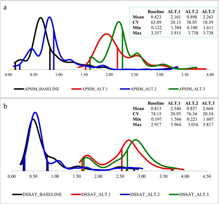
The yield distributions for all scenarios in the semi-arid and sub-humid agro-ecological zones of the Wami River sub-Basin are also presented in Fig. D1, Fig. D2 in Appendix D. The two models for both zones suggest that maize yield PDFs for ALT.1 and ALT.3 lie to the right of the PDFs for the BASELINE and ALT.2 scenarios. The ALT.2 yield PDF is not different from the BASELINE for the two models. Likewise, ALT.1 and ALT.3 yield PDFs are only slightly different except for DSSAT in the sub-humid area (Fig. D2-b).
3.2. Effect of alternative scenarios on maize net return
3.2.1. The semi-arid agro-ecological zone of the Wami River sub-basin
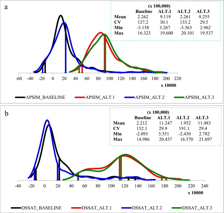
Table 5 shows the summary statistics of the effect of alternative scenarios on maize net returns per ha in the semi-arid area of the Wami River sub-Basin. The results on annual net income per ha for BASELINE in the semi-arid agro-ecological zone under both APSIM and DSSAT have a mean net return of TZS 226,000 and TZS 221,000 with a negative minimum value of TZS –316,000 and TZS –209,000 respectively. The probability of negative net returns (Prob (π<0)) is higher for ALT.2 and BASELINE scenarios because net returns were not enough to pay for the added seed. The maximum value is TZS 1 632,000 for APSIM and TZS 1 499,000 for DSSAT. ALT.2 has slightly different from the BASELINE in terms of mean, minimum, and maximum annual net returns (Table 5). ALT.1 and ALT1.3 have greater net returns than the BASELINE with a mean of more than TZS 900,000 and TZS 1,000,000 for APSIM and DSSAT. The minimum net return for ALT.1 and ALT.3 is TZS 327,000 and TZS 296,000, with the maximum values of TZS 1960,000 and TZS 1954,000 for APSIM respectively. DSSAT has a minimum of about TZS 355,000 and TZS 278,000, with the maximum amount of over TZS 2,000,000 for ALT.1 and ALT.3. The relative risk associated with the annual average net return is higher for the BASELINE (127.2% for APSIM and 152.1% for DSSAT) and ALT.2 (133.2% for APSIM and 191.1% for DSSAT). The relative variability about the mean is less than 31% for ALT.1 and ALT.3 for both DSSAT and APSIM.
Table 5.
Summary statistics for annual maize net return (TZS hundred thousand) in semi-arid.
| APSIM |
DSSAT |
|||||||
|---|---|---|---|---|---|---|---|---|
|
BASELINE |
ALT.1 |
ALT.2 |
ALT.3 |
BASELINE |
ALT.1 |
ALT.2 |
ALT.3 |
|
| TZS/ha | TZS/ha | TZS/ha | TZS/ha | TZS/ha | TZS/ha | TZS/ha | TZS/ha | |
| Mean | 226 | 912 | 226 | 925 | 221 | 1125 | 195 | 1148 |
| SD | 288 | 274 | 301 | 273 | 337 | 336 | 373 | 338 |
| CV | 127.2 | 30.1 | 133.2 | 29.5 | 152.1 | 29.9 | 191.1 | 29.4 |
| Min | −316 | 327 | −336 | 296 | −209 | 355 | −243 | 278 |
| Max | 1632 | 1960 | 2010 | 1954 | 1499 | 2044 | 1657 | 2170 |
| Prob(π<0) | 13.9% | – | 16.4% | – | 16.6% | – | 26.6% | – |
Fig. 3 represents the CDF for annual net returns in the semi-arid part of the basin for all the scenarios and models. The solid lines of the CDF are for APSIM and the square doted lines are for DSSAT. BASELINE and ALT.2 scenarios display negative values with non-negative values for ALT.1 and ALT.3. ALT.1 and ALT.3 scenarios lie to the right of the BASELINE and ALT.2 with a minor difference for the two scenarios, which indicates that the increased fertilizer scenarios produce higher net returns with less risk at each net returns level. DSSAT is slightly more to the right for ALT.1 and ALT.3, but the maximum and minimum values fall in the same range as APSIM. The baseline scenarios for both APSIM and DSSAT show a 13.9% and 16.6% probability of negative returns. The two models also suggest that ALT.2 has 16.4% and 26.6% probability of negative net returns and a zero probability for ALT.1 and ALT.3.
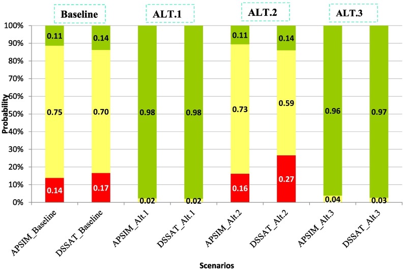
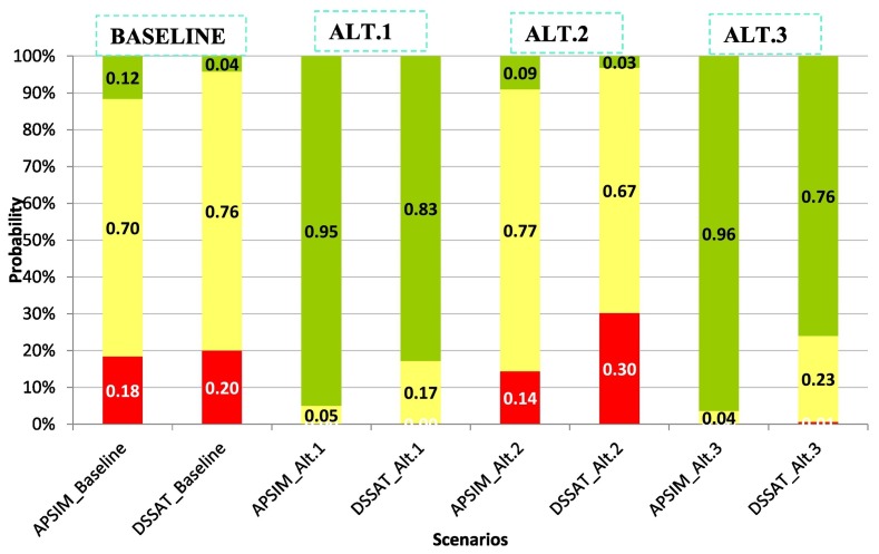
Fig. 4 is the Stoplight chart presenting the probabilities of the net return falling below zero and probabilities of being greater than the maximum target (TZS 500,000) for the farms in the semi-arid. The BASELINE scenarios for the APSIM and DSSAT models show a 14% and a 17% probability of negative annual net returns, respectively. The likelihood of BASELINE net return exceeding the maximum target of TZS 500,000 were 11% and 14%, with the probability of falling between the two targets being 75% and 70% for the two models. Both ALT.1 and ALT.3 have zero probability of net returns being negative and over 96% probability of exceeding the upper target for the two models. APSIM and DSSAT show that ALT.2 has 16% and 27% probability of net return being negative with the probability of exceeding the upper target net returns equaling the BASELINE.
Fig. 4.
Stoplight chart for probabilities of the annual net return being less than 0 and greater than TZS 500,000 thousand in the semi-arid part of the Wami River sub-basin.
The net income distributions of the alternatives in the semi-arid area are presented as PDFs in Fig. E1 (Appendix E). The PDFs suggest that the net income distributions for ALT.1 and ALT.3 are more favorable than the BASELINE and ALT.2 because they are further to the right. The BASELINE and ALT.2 scenario PDFs demonstrate the probabilities of negative net returns that is reported in the Stoplight chart (Fig. 4). The figures show that the net income distributions are further to the right and compared to the BASELINE and ALT.2. This difference implies that the relative variability of average net return is more likely to be lower for ALT.1 and ALT.3 than BASELINE and ALT.2, as demonstrated by the APSIM and DSSAT. For example, the relative variability of the average net return for BASELINE and ALT.2 scenarios is 4 to 5 times higher (127% to 152%) than ALT.1 and ALT.3 (29.9 to 30.1%) in the semi-arid area (Fig. E1-a).
3.2.2. The sub-humid agro-ecological zone of the Wami River sub-basin
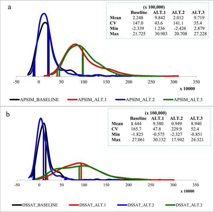
Table 6 presents the summary statistics for the effects of alternative scenarios on maize net returns in the sub-humid area. Likewise, APSIM results in a sub-humid agro-ecological zone of the basin report negative minimum net profits for the BASELINE and ALT.2 scenarios (Table 6). DSSAT also reports negative minimum returns for all the scenarios, with the risk being high for the BASELINE and ALT.2. The ALT.1 and ALT.3 scenarios have mean annual net returns of more than TZS 900,000 per ha for both APSIM and DSSAT. The CVs for ALT.1 and ALT.3 are relatively small compared to BASELINE and ALT.2. Although DSSAT demonstrated a negative return for all scenarios in the sub-humid area, the probability is less than 1.0% for ALT.1 and ALT.3 compared to BASELINE and ALT.2 with 20.2% and 30.2% respectively.
Table 6.
Summary statistics of the bio-economic simulation model on annual maize net return (TZS hundred thousand) in Sub-humid.
| APSIM |
DSSAT |
|||||||
|---|---|---|---|---|---|---|---|---|
|
BASELINE |
ALT.1 |
ALT.2 |
ALT.3 |
BASELINE |
ALT.1 |
ALT.2 |
ALT.3 |
|
| TZS/ha | TZS/ha | TZS/ha | TZS/ha | TZS/ha | TZS/ha | TZS/ha | TZS/ha | |
| Mean | 225 | 984 | 201 | 972 | 144 | 938 | 95 | 894 |
| SD | 330 | 429 | 284 | 344 | 239 | 449 | 218 | 469 |
| CV | 147.0 | 43.6 | 141.1 | 35.4 | 165.7 | 47.8 | 229.9 | 52.4 |
| Min | −234 | 124 | −243 | 288 | −183 | −58 | −233 | −85 |
| Max | 2173 | 3098 | 2071 | 2723 | 2706 | 3013 | 1794 | 2432 |
| Prob(π<0) | 18.6% | – | 14.6% | – | 20.2% | 0.4% | 30.2% | 0.7% |
Fig. 5 shows the CDF for annual net returns in the sub-humid area of the basin for all the scenarios both models. The BASELINE and ALT.2 CDFs lie entirely to the left of ALT.1 and ALT.3, implying that the two scenarios have a high probability of failure compared to ALT.1 and ALT.3 and that at each level of income the later scenarios have less risk. DSSAT demonstrated a 30% likelihood of negative returns for investing in ALT.2 with about 15% probability for APSIM. Also, the result shows that ALT.1 and ALT.3 have a zero chance of negative returns for APSIM with 0.4% and 0.7% probability of negative returns for DSSAT. Fig. E2 in Appendix E presents the sub-humid area results as CDFs and suggests that returns distributions for ALT.1 and ALT.3 are more to the right of the BASELINE and ALT.2 for the two models.
Fig. 5.
CDF of annual net return in sub-humid as for APSIM and DSSAT cropping models.
Fig. 6 is a Stoplight chart presenting the probability of annual net returns being below, above or between TZS 0 and TZS 500,000 in the sub-humid area. The BASELINE under the bio-economic simulation model for both APSIM and DSSAT has 18% and 20% probability of negative net returns. The ALT.1 and ALT.3 have zero probability of negative annual net returns for the two crop models. APSIM and DSSAT results indicate a 14% and 30% probability of negative returns for ALT.2. ALT.1 and ALT.3 have the highest probability of net return exceeding the upper target of TZS 500,000. For example, APSM yield are associated with 95% and 96% probabilities that the net returns would exceed the upper target, while DSSAT yields are associated with 83% and 76% probabilities for ALT.1 and ALT.3. Of all the scenarios in the sub-humid basin, ALT.2 has the smallest probability of net revenue being above the upper target for the two models.
Fig. 6.
Stoplight chart for probabilities of the annual net return being less than 0 and greater than TZS 500,000 thousand in sub-humid part of the Wami River sub-basin.
3.2.3. The economic feasibility of the selected options across agro-ecological zones
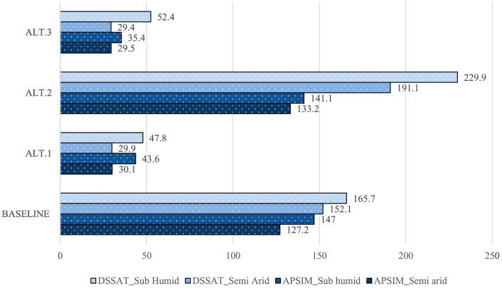
The simulation results in the baseline scenario (BASELINE) for both APSIM and DSSAT confirmed that the sub-humid area has higher probabilities of negative net returns than the semi-arid region. APSIM estimated 18.6% probability of negative net returns for the sub-humid and 13.9% for the semi-arid, with DSSAT estimating 20.2% and 16.6% probabilities for the two zones. When farms are supplemented with ALT.1, the two bio models suggest a zero probability of negative net returns for both zones except DSSAT in the sub-humid area. DSSAT estimated a small chance (0.4%) of negative net returns. Under ALT.2, both models suggest a negative net return for all the agro-ecological zones with sub-humid having the most risk. When the two interventions are applied together (ALT.3), both yield models suggest a zero probability of negative net returns, but DSSAT displayed a small probability of 0.7% that the net returns will fall below zero. Although the sub-humid area has the highest maximum net returns, the relative risk measured by the CVs is higher than the semi-arid (Fig. 7 ).
Fig. 7.
Coefficient of variation (CV) of net returns for the semi-arid and sub-humid area in Wami River sub-basin.
Overall results of the economic feasibility assessment of 40 kg N/ha (ALT.1) and 3.3 plants/m2 (ALT.2) for maize yield in Wami River sub-Basin, Tanzania indicate that it is worth investing in ALT.1. The farms that adopt ALT.2 as a standalone intervention do not work better for the semi-arid and sub-humid agro-ecological zones within the Wami River sub-Basin. Also, ALT.3, which combines ALT.1 and ALT.2, does not result in a significant difference from the application of ALT.1 alone. Hence, a rational farmer may use ALT.1 only because ALT.3 would lead to a higher production cost without an increase in net returns.
Our results are in line with many studies to assess the influence of agronomic practices on the maize sub-sector. Some of these studies include Msongaleli et al. (2015), Beletse et al. (2015), Masikati et al. (2015), Mwinuka et al., 2016, Mwinuka et al., 2017, and Rao et al. (2015). Although these studies did not clearly elaborate on the economic contribution of fertilizer application, they argued that N-fertilizer's use could be one of the fundamental alternatives to reducing risks and uncertainties, especially given climate variability. The studies also claimed that besides the fertilizers' application, adjustments in planting densities should not be ignored.
Additionally, our study agrees with Walker and Schulze (2006), who reported that agronomic practices, especially fertilizer applications, have a more considerable influence, on reducing uncertainty in agricultural production systems. Wilson and Lewis (2015) highlighted that the low production of maize in Tanzania is influenced by limited use of modern inputs like nitrogen fertilizers, which is currently ranging between 9 and 16 kg/ha/year. The low utilization of the N-fertilizer has led to higher uncertainties and lower performance of the sub-sector. Mourice et al. (2014; ) concluded that small nitrogen fertilizer doses would still be beneficial for resource-poor farmers through higher grain yields. However, the Agriculture Climate Resilience Plan (ACRP) 2014–2019 of Tanzania warned that interventions such as improving planting density and the use of fertilizer to increase productivity could show positive outcomes if properly implemented (URT, 2014).
4. Conclusions
The purpose of this paper was to contribute to the existing literature a new framework for integrating different biophysical models into economic perspectives in SSA, particularly Tanzania. A bio-economic simulation model was demonstrated under the Monte Carlo simulation protocol for evaluating the economic viability of risk reducing interventions proposed for maize production. Thus, a stochastic bio-economic simulation model of 168 maize plots in the Wami River sub-Basin was developed based on data from two crop models (APSIM and DSSAT). Stochastic values for production costs and prices were incorporated into the model to assess the probable annual net return of maize sub-sector under two crop management alternatives.
First, the Monte Carlo simulation techniques were used to convert the yields from the biophysical models into a stochastic state to capture the risk and uncertainties associated with the yields. Second, the Monte Carlo simulated yields for the baseline and alternatives were validated to ensure that the random variables are simulated correctly. Thirdly, the stochastic annual price of maize was combined with the stochastic yields to simulate stochastic annual revenue. Lastly, the total costs for the baseline and alternatives were used to simulate the empirical distribution of net returns for each scenario. PDFs, CDFs, Tables, and Stoplight charts were developed to rank the targeted options.
Our results suggest that an increase in plant population of 33,000 plants/ha alone, particularly in the Wami River sub-Basin, would have no significant difference in annual net returns from the current maize productivity compared to the application of 40 kg N-fertilizers per ha. In terms of profitability, our bio-economic simulation results suggest an increase in net farm return of up to fivefold when farms are supplemented with the N-fertilizer. Increasing the plant population within the Wami River sub-Basin will likely not increase annual net returns from the baseline unless the two practices are applied concurrently.
The results suggest the importance of emphasizing the application of crop management strategies, especially using at least 40 kg N/ha rate of fertilizers. The economic returns were higher for increased fertilizer application than from increasing plant population. The application of fertilizers may accelerate to achieving improved food availability and reduced poverty to maize-based producers in Tanzania who are mainly small-scale farmers. Moreover, the study contributes to the National Agricultural Policy and the Agriculture Climate Resilience Plan (ACRP) 2014–2019 of Tanzania. For example, the ACRP plan has one of its key messages: “alternative technologies should focus on boosting cereal crops' productivity to increase yields, enhance food security, and reduce poverty to smallholder farmers.”
This study analyzed only two management practices, namely N-fertilizer application and plant population adjustment. There is a need for similar studies on risk reducing alternatives that could potentially boost productivity and profitability in Tanzania and the rest of SSA. The methodology used in this study was used to assess the economic feasibility of only two technology packages by employing data from two crop models to develop a bio-economic simulation model in a stochastic environment. We argue that the procedures expressed in this study form a basis for more research and include more agricultural practices/technologies that claim to boost productivity, enhance food security, and reduce poverty among the majority of the poor. Similar studies are needed given the dearth of integrated assessments that capture agricultural risks by linking appropriate biophysical and economics models. The integrated assessment can improve decision-making for policy-makers and farmers in Tanzania and the rest of SSA.
Declaration of Competing Interest
The authors declare that they have no conflict of interests in relation to this paper.
Acknowledgments
This work was sponsored by IDRC-AARC regional collaborative research project entitled “Enhancing Climate Change Adaptation in Agriculture and Water Resources in the Great Horn of Africa” led by the Soil–Water Management Research Programme at the Sokoine University of Agriculture and supported by the UKaid grant GB-1-202108 to the Agricultural Model Inter-comparison and Improvement Project (AgMIP) and collaborators. The Article Processing Charge was Funded by the Leibniz Centre for Agricultural Landscape Research (ZALF). The study was conducted within the AgMIP Protocols and Regional Integrated Assessments (www.agmip.org). The authors would like to acknowledge the contribution of Dr. Roberto O. Valdivia and Professor John Antle for their time training the AgMIP Protocols. The study used the existing biophysical data sets prepared during the first and second phases of the AgMIP project from 2012 to 2016. The first author also expresses his gratitude to the Agricultural and Food Policy Center at Texas A&M University (https://www.afpc.tamu.edu) under the Feed the Future Innovation Lab for Small-Scale Irrigation Project (ILSS) for conducting specialized training on the Monte Carlo simulation from which this paper benefited enormously. Views expressed here are the authors' own, as all errors and omissions.
The authors declare that they have no conflict of interests in relation to this paper.
Appendix A. Data validation for the observed and baselines
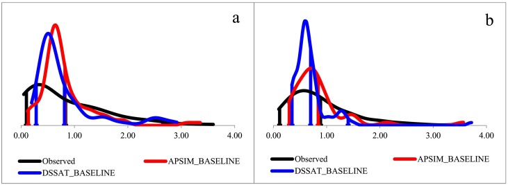
This Appendix presents data validation for the observed and baselines from the process-based models for semi-arid and sub-humid agro-ecological zones of the Wami River sub-Basin. This validation Table A1 displays maize yield summary statistics in terms of mean, standard deviation (SD), coefficient of variation (CV), minimum, maximum yields for the observed and baseline data sets. The two models produce PDFs similar to the observed with APSIM being closer, making the data from the two models suitable for economic analysis Fig. A1.
Table A1.
Summary statistics for observed and baseline maize yields in the basin.
| Semi-arid |
Sub-humid |
|||||
|---|---|---|---|---|---|---|
| Observed |
APSIM_baseline |
DSSAT_baseline |
Observed |
APSIM_baseline |
DSSAT_baseline |
|
| t/ha | t/ha | t/ha | t/ha | t/ha | t/ha | |
| Mean | 0.836 | 0.823 | 0.813 | 0.885 | 0.841 | 0.697 |
| SD | 0.758 | 0.533 | 0.607 | 0.640 | 0.561 | 0.416 |
| CV | 90.71 | 64.70 | 74.61 | 72.23 | 66.78 | 59.71 |
| Min | 0.500 | 0.683 | 0.564 | 0.100 | 0.286 | 0.346 |
| Max | 3.600 | 3.357 | 2.916 | 3.500 | 3.568 | 3.719 |
| Sample | 83 | 83 | 83 | 85 | 85 | 85 |
Fig. A1.
Probability distribution function (PDF) of the observed and baselines of the APSIM and DSSAT for semi-arid (a) and sub-humid (b).
Appendix B. Data validation for process-based data vs. Monte Carlo bio-economic simulation model in the semi-arid area of the Wami River sub-Basin
This Appendix provides the statistical tests used to validate that the Monte Carlo bio-economic simulation procedures reproduce the process-based data. A Student's-t-test was used to test that Monte Carlo bio-economic simulated means () is not statistically different from the process-based means (). The validation results are shown in Table B1. The results for t-Test of the means for the yield for each scenario indicated that the Monte Carlo bio-economic simulated means are statistically equal to the deterministic means at the 95% level. All of the test statistics (test values) are less than the critical value of 2.25 for each scenario, and the p-values are >0.1 at the alpha equal to 5% (p > .05) thus we failed to reject the null hypothesis that the means are equal (Table B1). The validation tests for semi-arid have similar results, hence based on the evaluation tests, the Monte Carlo simulated yields can be used for bio-economic modeling. The null and alternative hypotheses for the Student's-t-test are as follows:
Table B1.
Statistical validation test to determine the bio-economic simulation procedures for sub-humid area.
| Test Parameters (Test for simulated vs deterministic means) |
||||||||
|---|---|---|---|---|---|---|---|---|
| Confidence Level | 95.0000% | Critical Value | 2.25 | |||||
| 83 process-based mean yield vs. 500 Monte Carlo mean yield for APSIM_BASELINE | ||||||||
| Given Value | Test Value | P-Value | ||||||
| t-Test | 0.841 | 0.004 | 0.997 | Fail to Reject the Ho that the Mean is Equal to 0.8405 | ||||
| 83 process-based mean yield vs. 500 Monte Carlo mean yield for APSIM_ALT.1 | ||||||||
| Given Value | Test Value | P-Value | ||||||
| t-Test | 2.379 | 0.003 | 0.998 | Fail to Reject the Ho that the Mean is Equal to 2.3795 | ||||
| 83 process-based mean yield vs. 500 Monte Carlo mean yield for APSIM_ALT.2 | ||||||||
| Given Value | Test Value | P-Value | ||||||
| t-Test | 0.889 | −0.014 | 0.989 | Fail to Reject the Ho that the Mean is Equal to 0.8891 | ||||
| 83 process-based mean yield vs. 500 Monte Carlo mean yield for APSIM_ALT.3 | ||||||||
| Given Value | Test Value | P-Value | ||||||
| t-Test | 2.439 | 0.017 | 0.986 | Fail to Reject the Ho that the Mean is Equal to 2.4389 | ||||
| 83 process-based mean yield vs. 500 Monte Carlo mean yield for DSSAT_BASELINE | ||||||||
| Given Value | Test Value | P-Value | ||||||
| t-Test | 0.697 | 0.011 | 0.991 | Fail to Reject the Ho that the Mean is Equal to 0.6974 | ||||
| 83 process-based mean yield vs. 500 Monte Carlo mean yield for DSSAT_ALT.1 | ||||||||
| Given Value | Test Value | P-Value | ||||||
| t-Test | 2.301 | 0.017 | 0.986 | Fail to Reject the Ho that the Mean is Equal to 2.3014 | ||||
| 83 process-based mean yield vs. 500 Monte Carlo mean yield for DSSAT_ALT.2 | ||||||||
| Given Value | Test Value | P-Value | ||||||
| t-Test | 0.689 | 0.011 | 0.991 | Fail to Reject the Ho that the Mean is Equal to 0.6889 | ||||
| 83 process-based mean yield vs. 500 Monte Carlo mean yield for DSSAT_ALT.3 | ||||||||
| Given Value | Test Value | P-Value | ||||||
| t-Test | 2.292 | −0.007 | 0.994 | Fail to Reject the Ho that the Mean is Equal to 2.2923 | ||||
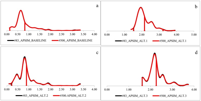
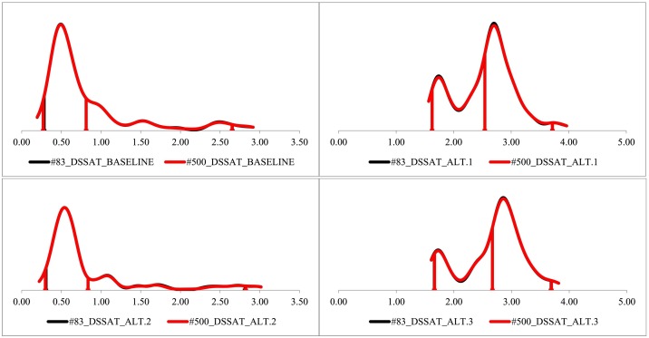
Likewise, this Appendix presents data validation for the alternative scenarios from the process-based data against the 500 bio-economic simulation data for two agro-ecological zones of the Wami River sub-Basin. The two process-based models produce PDFs (black PDFs) similar to the bio-economic simulated data (red PDFs) for the baseline, ALT.1, ALT.2 and ALT.3 scenarios. (Note the red line distributions are on top of the black line distributions for most all points.) The similarities in the charts suggest that bio-economic simulated data under Monte Carlo simulation procedures reproduce the process-based data set parameters. Fig. B1, Fig. B2 are data sets for APSIM and DSSAT respectively.
Fig. B1.
Data validation of 83 maize plots for APSIM process-based data (in Black PDFs) vs. 500 iterations bio-economic simulated data (in Red PDFs) in the semi-arid zone. (For interpretation of the references to colour in this figure legend, the reader is referred to the web version of this article.)
Fig. B2.
Data validation of 83 maize plots for DSSAT process-based data (in Black PDFs) vs. 500 iterations bio-economic simulated data (in Red) in the semi-arid zone. (For interpretation of the references to colour in this figure legend, the reader is referred to the web version of this article.)
Appendix C. Distribution of costs for the baseline scenario in the basin (TZS/ha)
This Appendix displays the per ha costs incurred by smallholder farmers for different operations in maize production in the Wami River sub-Basin. A uniform probability distribution was used to simulated stochastic/random production costs using the = UNIFORM() function in Simetar. The function of production cost for the baseline scenario was programmed using Eq. C1 as follows:
| (C1) |
where: k represents all cost items including land preparation, seeds, planting, ... and postharvest handling,
Min is the minimum value for the distribution,
Max is the maximum value for the distribution,
The stochastic cost for the baseline scenario was therefore combined with additional costs of 40 kg N/ha (ALT.1) and 7–10 kg of maize seeds (ALT.2). The total cost for ALT.3 was calculated by adding the baseline costs to cost for ALT.1 and ALT.2.
Table C1.
Budgets for maize production per ha in Wami River sub-Basin for the year 2015/16.
| Minimum cost (TZS/ha) | Maximum cost (TZS/ha) | |
|---|---|---|
| Land preparation | 25,000 | 50,000 |
| Seeds | 60,000 | 70,000 |
| Planting | 20,000 | 30,000 |
| Weeding | 30,000 | 50,000 |
| Fertilizers | 0 | 50,000 |
| Fertilizer application | 0 | 20,000 |
| Pesticides | 0 | 14,000 |
| Pesticides application | 0 | 6000 |
| Harvesting | 5000 | 20,000 |
| Postharvest handling (transportation and storage) | 15,000 | 50,000 |
| Total cost | 150,000 | 360,000 |
Fig. C1.
PDF of total production cost per ha, by scenario in the bio-economic model.
Source: Computed from the survey data.
Appendix D. Maize yield distribution for baseline and alternative scenarios in Wami River-sub basin
Appendix D, shows the schematic presentation of annual maize yields for baseline and alternative scenarios in the semi-arid part (Fig. D1) and sub-humid part (Fig. D2) of the Wami River sub-Basin. Fig. D1-a and Fig. D2-a shows the yield distribution for APSIM cropping system model and for DSSAT cropping system is represented by Fig. D1-b and D2-b.
Fig. D1.
PDF of annual maize yields for the baseline and alternative scenarios in the semi-arid part of the Wami River sub-Basin: a = APSIM cropping system model and b = DSSAT cropping system model.
Fig. D2.
PDF of annual maize yields for the baseline and alternative scenarios in a sub-humid part of the Wami River sub-Basin: a = APSIM cropping system model and b = DSSAT cropping system model.
Appendix E. Income distribution for baseline and alternative scenarios in Wami River sub-basin
Appendix E, shows the schematic presentation of annual maize income for the baseline and alternative scenarios in the semi-arid part (Fig. E1) and sub-humid part (Fig. E2) of the Wami River sub-Basin. Fig. E1-a and Fig. E1-b shows the net return distributions for APSIM and DSST cropping system models in semi-arid part of the Wami River sub-Basin respectively. The CVs in this model measure the relative risk (relative variability) associated with net return. Both BASELINE and ALT.2, show negative net return with non-zero values for ALT.1 and ALT.3. Also, the relative variabilities about the average net return are higher for BASELINE (127% & 152%), and ALT.2 (133% & 191%) for both APSIM and DSSAT cropping models, respectively. In contrast, ALT.1 (30.1% & 29.9%) and ALT.3 (29.5% & 29.4%) have the smallest values of CVs, hence lower relative risk associated with net return.
Fig. E1.
PDF of annual maize net return per ha for baseline and alternative scenarios in the semi-arid part of the Wami River sub-Basin: a = APSIM cropping system model and b = DSSAT cropping system model.
Fig. E2-a and Fig. E2-b shows the net return distribution for APSIM and DSST cropping system models in sub-humid part of the Wami River sub-Basin respectively. DSSAT presents negative minimum values for all the scenarios with the BASELINE and ALT.2 having the highest risk associated with net return. Likewise, the CVs are higher for BASELINE, and ALT.2 and less for the ALT.1 and ALT.3.
Fig. E2.
PDF of annual maize net return per ha for the baseline and alternative scenarios in a sub-humid part of the Wami River sub-Basin: a = APSIM cropping system model and b = DSSAT cropping system model.
References
- Ahmed M., Hassan F.U. 19th International Congress on Modelling and Simulation, Perth, Australia. 2011. APSIM and DSSAT models as decision support tools; pp. 12–16. [Google Scholar]
- Beletse Y.G., Durand W., Nhemachena C., Crespo O., Tesfuhuney W.A., Jones M.R., Teweldemedhin M.Y., Gamedze S.M., Bonolo P.M., Jonas S., Walker S. 2015. Projected Impacts of Climate Change Scenarios on the Production of Maize in Southern Africa. An integrated assessment case study of the bethlehem district; pp. 125–157. Central Free State, South Africa. [Google Scholar]
- Bizimana J.C., Richardson J.W. Agricultural technology assessment for smallholder farms: an analysis using a farm simulation model (FARMSIM) Comput. Electron. Agric. 2019;156:406–425. [Google Scholar]
- Feder G., Just R.E., Zilberman D. Adoption of agricultural innovations in developing countries: a survey. Econ. Dev. Cult. Chang. 1985;33(2):255–298. [Google Scholar]
- Hoogenboom G., Porter C.H., Shelia V., Boote K.J., Singh U., White J.W., Hunt L.A., Ogoshi R., Lizaso J.I., Koo J., Asseng S., Singels A., Moreno L.P., Jones J.W. DSSAT Foundation; Gainesville, Florida, USA: 2017. Decision Support System for Agrotechnology Transfer (DSSAT) version 4.7 (https://DSSAT.net) [Google Scholar]
- IFDC Tanzania Fertilizer Assessment. 2012. https://africafertilizer.org/en/blog-post/tanzania-fertilizer-market-assessment-ifdc-afap-june-2012 Available at.
- Jones J.W., Keating B.A., Porter C.H. Approaches to modular model development. Agric. Syst. 2001;70:421–443. [Google Scholar]
- Jones J.W., Hoogenboom G., Porter C.H., Boote K.J., Batchelor W.D., Hunt L.A., Wilkens P.W., Singh U., Gijsman A.J., Ritchie J.T. DSSAT cropping system model. Eur. J. Agron. 2003;18:235–265. [Google Scholar]
- Kadigi I.L., Richardson J.W., Mutabazi K.D., Philip D., Bizimana J.C., Mourice S.K., Waized B. Forecasting yields, prices and net returns for main cereal crops in Tanzania as probability distributions: a multivariate empirical (MVE) approach. Agric. Syst. 2020;180:102693. [Google Scholar]
- Kahimba F.C., Sife A.S., Maliondo S.M.S., Mpeta E.J., Olson J. Climate change and food security in Tanzania: analysis of current knowledge and research gaps. Tanzania J. Agric. Sci. 2015;14(1) [Google Scholar]
- Keating B.N., Carberry P.S., Smith C.J. An overview of APSIM, a model design for farming systems simulation. Eur. J. Agron. 2003;18:267–272. [Google Scholar]
- Macauley H., Ramadjita T. Cereal crops: rice, maize, millet, sorghum, wheat. Feeding Afr. 2015;36 https://www.afdb.org/fileadmin/uploads/afdb/Documents/Events/DakAgri2015/Cereal_Crops-_Rice__Maize__Millet__ Sorghum__Wheat.pd site visited on 15/10/2018. [Google Scholar]
- Masikati P., Tui S.H.K., Descheemaeker K., Crespo O., Walker S., Lemard C.J., Claessens L.F.G., Gama A.C., Famba S., van Rooyen A.F., Valdivia R.O. Handbook of Climate Change and Agroecosystems. 2015. Crop–livestock intensification in the face of climate change: exploring opportunities to reduce risk and increase resilience in southern Africa by using an integrated multi-modeling approach’; pp. 159–198. [Google Scholar]
- McCown R.L., Hammer G.L., Hargreaves J.N.G., Holzworth D.P., Freebairn D.M. APSIM: a novel software system for model development, model testing, and simulation in agricultural systems research. Agric. Syst. 1996;50:255–271. [Google Scholar]
- Mourice S.K., Rweyemamu C.L., Tumbo S.D. Narrowing maize yield gaps under rain-fed conditions in Tanzania: effect of small nitrogen dose. Tanzania J. Agric. Sci. 2014;12(2):55–65. [Google Scholar]
- Msongaleli B.M., Rwehumbiza F., Tumbo S.D., Kihupi N. Impacts of climate variability and change on rainfed sorghum and maize: implications for food security policy in Tanzania. J. Agric. Sci. 2015;7(5):124–142. doi: 10.5539/jas.v7n5p124. [DOI] [Google Scholar]
- Mwinuka L., Mutabazi K.D., Makindara J., Sieber S. Reckoning the risks and rewards of fertilizer micro-dosing in a sub-humid farming system in Tanzania. Afr. J. Sci. Technol. Innov. Dev. 2016;8(5–6):497–508. [Google Scholar]
- Mwinuka L., Mutabazi K.D., Sieber S., Makindara J., Bizimana J.C. An economic risk analysis of fertiliser microdosing and rainwater harvesting in a semi-arid farming system in Tanzania. Agrekon. 2017;56(3):274–289. [Google Scholar]
- NBS – National Bureau of Statistics Tanzania National Panel Survey Report - Wave 2. 2012. https://www.nbs.go.tz/nbs/takwimu/nps/NPS_Report-2010-2011.zip 2010–2011. site visited on 20/01/2015.
- Palma M.A., Richardson J.W., Roberson B.E., Ribera L.A., Outlaw J., Munster C. Economic feasibility of a mobile fast pyrolysis system for sustainable bio-crude oil production. Int. Food Agribusiness Manag. Rev. 2011;14(3):1–16. [Google Scholar]
- Rao K.P., Gummadi S., Mulwa R.M., Kilavi M.N., Esilaba A., Athanasiadis I.N. Handbook of Climate Change and Agroecosystems. Vol. 3. 2015. Impacts of climate variability and change on agricultural systems in Eastern Africa; pp. 75–124. [Google Scholar]
- Rezende M.L., Richardson J.W. Economic feasibility of sugar and ethanol production in Brazil under alternative future prices outlook. Agric. Syst. 2015;138:77–87. [Google Scholar]
- Richardson, J.W., and Bizimana, J.C. (2017). Agricultural Technology Assessment for Smallholder Farms in Developing Countries: An Analysis using a Farm Simulation Model (FARMSIM). Working paper. [https://afpc.tamu.edu/research/publications/683/FARMSIM.pdf] site visited on 21/03/2018.
- Richardson J.W., Klose S.L., Gray A.W. An applied procedure for estimating and simulating multivariate empirical (MVE) probability distributions in farm-level risk assessment and policy analysis. J. Agric. Appl. Econ. 2000;32(02):299–315. [Google Scholar]
- Richardson J.W., Schumann K.D., Feldman P.A. Agricultural and Food Policy Center, Department of Agricultural Economics, Texas A&M University; College Station, TX: 2008. Simetar: Simulation and econometrics to analyze risk. [Google Scholar]
- Rosenzweig C., Jones J., Antle J., Hatfield J. Protocols for AgMIP Regional Integrated Assessments, Version 6.0. 2015. http://www.agmip.org/wp-content/uploads/2015/09/AgMIP-RIA-Protocols-V6sm.pdf site visited on 30/06/2017.
- Rötter R.P., Carter T.R., Olesen J.E., Porter J.R. Crop-climate models need an overhaul. Nat. Clim. Chang. 2011;1(4):175–177. [Google Scholar]
- The World Bank Fertilizer Consumption (kilograms per hectare of arable land) – Tanzania. 2020. https://data.worldbank.org/indicator/AG.CON.FERT.ZS?locations=TZ Retrieved from.
- Thompson H.E., Berrang-Ford L., Ford J.D. Climate change and food security in sub-Saharan Africa: a systematic literature review. Sustainability. 2010;2(8):2719–2733. [Google Scholar]
- Tumbo S., Mzirai O., Mourice S., Msongaleli B., Wambura F., Kadigi I.…Mutabazi K. 2015. Assessing the Impacts of Climate Variability and Change on Agricultural Systems in Eastern Africa while Enhancing the region's Capacity to Undertake Integrated Assessment of Vulnerabilities to Future Changes in Climate-Tanzania. (Research gate) [Google Scholar]
- Tumbo S.D., Mutabazi K.D., Mourice S.K., Msongaleli B.M., Wambura F.J., Mzirai O.B., Kadigi I.L., Kahimba F.C., Mlonganile P., Ngongolo H.K., Sangalugembe C. Climate Variability and Change in Africa. Springer; Cham: 2020. Integrated assessment of climate change impacts and adaptation in agriculture: the case study of the Wami River Sub-Basin, Tanzania; pp. 115–136. [Google Scholar]
- URT – The United Republic of Tanzania National Adaptation Programme of Action (NAPA). Division of Environment, Vice President's Office, Dar es Salaam. 2007. https://unfccc.int/resource/docs/napa/tza01.pdf site visited on 17/06/2016.
- URT – The United Republic of Tanzania The United Republic of Tanzania: National Agriculture Policy. 2013. http://www.tzdpg.or.tz/fileadmin/documents/dpg_internal/dpg_working_groups_clusters/cluster_1/agriculture/2._Ag_policies_and_strategies/National_ag_policies/1._2013_NATIONAL_AGRICULTURAL_POLICY_-_FINALFebruari_2013.pdf Dar Es Salaam. Available at: site visited on 12/07/2017.
- URT – The United Republic of Tanzania Ministry of Agriculture, Food Security, and Cooperatives: Agriculture Climate Resilience Plan 2014–2019. 2014. http://extwprlegs1.fao.org/docs/pdf/tan152483.pdf site visited on 14/06/2016.
- URT – The United Republic of Tanzania Climate-Smart Agriculture Guideline of the United Republic of Tanzania. 2017. http://www.kilimo.go.tz/uploads/regulations/National_CSA_Guideline.pdf Available at: site visited on 12/07/2017.
- URT – United Republic of Tanzania Agricultural Sector Development Programme Phase Two (ASDP II) 2016. http://www.tzdpg.or.tz/fileadmin/documents/external/national_development_frameworks/ASDP2_Final_Document_20_May._2016__after_edit__1_.pdf site visited on 12/10/2018.
- Waithaka M., Nelson G.C., Thomas T.S., Kyotalimye M., editors. East African agriculture and climate change: a comprehensive analysisWashington, D.C.: International Food Policy Research Institute (IFPRI) 2013 doi: 10.2499/9780896292055. [DOI] [Google Scholar]
- Walker N.J., Schulze R.E. An assessment of sustainable maize production under different management and climate scenarios for smallholder agro-ecosystems in KwaZulu-Natal, South Africa. Phys. Chem. Earth, Parts A/B/C. 2006;31(15–16):995–1002. [Google Scholar]
- White J.W., Hoogenboom G., Kimball D.A., Wall G.W. Methodologies for simulating impacts of climate change on crop production. Field Crop Res. 2011;124(3):357–368. [Google Scholar]
- Wilson R.T., Lewis J. The Maize Value Chain in Tanzania. 2015. https://saiia.org.za/wp-content/uploads/2016/06/008-Tanzania_maize.pdf site visited 15/11/2018.
- Wolday K., Hruy G. A review: performance evaluation of crop simulation model (APSIM) in prediction crop growth, development and yield in semi-arid tropics. J. Nat. Sci. Res. 2015;5(21):34–39. [Google Scholar]


