Kalman Filter–Based Microbubble Tracking for Robust Super-Resolution Ultrasound Microvessel Imaging

Abstract

Contrast microbubble-based super-resolution ultrasound microvessel imaging (SR-UMI) overcomes the compromise in conventional ultrasound imaging between spatial resolution and penetration depth, and has been successfully applied to a wide range of clinical applications. However, clinical translation of SR-UMI remains challenging due to the limited number of microbubbles (MBs) detected within a given accumulation time. Here we propose a Kalman filter-based method for robust MB tracking and improved blood flow speed measurement with reduced numbers of MBs. An acceleration constraint and a direction constraint for MB movement were developed to control the quality of the estimated MB trajectory. An adaptive interpolation approach was developed to inpaint the missing microvessel signal based on the estimated local blood flow speed, facilitating more robust depiction of microvasculature with a limited amount of MBs. The proposed method was validated on an ex ovo chorioallantoic membrane and an in vivo rabbit kidney. Results demonstrated improved imaging performance on both microvessel density maps and blood flow speed maps. With the proposed method, the percentage of microvessel filling in a selected blood vessel at a given accumulation period was increased from 28.17% to 74.45%. A similar SR-UMI performance was achieved with MB numbers reduced by 85.96%, compared to that with the original MB number. The results indicate that the proposed method substantially improves the robustness of SR-UMI under a clinically relevant imaging scenario where SR-UMI is challenged by a limited MB accumulation time, reduced number of MBs, lowered imaging frame rate, and degraded signal-to-noise ratio.

I. Introduction

THE emerging field of contrast microbubble-based super-resolution ultrasound microvessel imaging (SR-UMI) has been evolving rapidly [1–9]. The unprecedented combination of imaging resolution and penetration depth opens new possibilities for a wide range of clinical applications, including cancer [5, 10–12] and functional neural imaging [1]. At present, however, clinical translation of SR-UMI remains challenging due to a number of hurdles, such as tissue motion [13], low microbubble (MB) signal-to-noise-ratio (SNR) in vivo [14, 15], incomplete sampling of MB signal using two dimensional (2D) imaging [16], and a limited number of MBs detected within a given accumulation time [17]. While most of these challenges can be mitigated by translating the imaging scheme to 3D, thanks to the latest development on sparse array and sparse synthetic aperture beamforming [18–20], MB signal accumulation is fundamentally limited by restrictions of clinical MB dose and physiology (e.g., slow microvasculature perfusion requires long accumulation time of MBs). In addition, part of the detected MB signal has to be discarded due to the presence of imaging noise and tissue motion in in vivo applications, which exacerbates the problem of inadequate MB signal, resulting in discontinuous microvascular depiction and unreliable flow speed estimation [1, 17]. To alleviate this issue, we previously proposed a linear interpolation-based method to restore the missing data points of an MB movement trajectory and recover the continuous microvessel signal [14]; this was termed “inpainting” in the previous work. While linear interpolation greatly improved the appearance of the SR-UMI microvessel density and flow speed maps, this method assumed constant MB flow speed at a vascular tree in a short time duration, which may be violated in practice. Also, the interpolation method did not consider any mechanisms for checking MB tracking fidelity; therefore, it may have been easily biased by inaccurate MB locations that resulted from upstream processing. Thus, the objective of this study was to improve upon the previous linear interpolation method and develop better tracking and inpainting approaches for robust SR-UMI.

To achieve this goal, we investigated the use of Kalman filtering for MB tracking in SR-UMI. A Kalman filter is a well-established algorithm that uses a series of measurements observed over time which contain statistical noise and measurement inaccuracies. The filter then uses these measurements to predict the status of variables [21]. By estimating a joint probability distribution over the variables for each timeframe, Kalman-filtered measurements are more accurate than those based on single measurements. Kalman filtering has been widely used in solving navigation problems, guidance and control of vehicles, aircraft, and spacecraft. Since MB tracking is similar to vehicle tracking, Kalman filtering was first adopted for MB aided ultrasound imaging in [8] and [9]. However, the Kalman filter was used as one of many components in a large network of their MB localization and tracking algorithms.

Our hypothesis was that Kalman filter-based MB tracking can significantly improve the tracking accuracy of MB trajectory. Meanwhile, we took advantage of physiological behaviors of MB movements and developed two constraints to further reject false MB locations and movement trajectories after Kalman filtering. In addition, an advanced inpainting technique based on adaptive interpolation was developed to recover the missing microvessel data points and substantially improve the visual appearance and accuracy of SR-UMI. The method was validated on both an ex ovo chorioallantoic membrane (CAM) model and on an in vivo rabbit kidney model. The rest of the paper is structured as follows: in the Materials and Methods section, we introduce the SR-UMI processing workflow, followed by detailed descriptions of the ex ovo and in vivo experiment setups. We then show results for each procedure of the proposed method, as well as the comparison of before and after processing. We finalize the paper with Discussion and Conclusions.

II. Methods

A. Data processing for SR-UMI

Figure 1 summarizes the in-phase quadrature-phase (IQ) data processing chain with the Kalman filter-based MB tracking for SR-UMI. The method for extracting an isolated MB signal used in this study was similar to previously reported methods [1, 14, 15]. First, an optimized phase correlation-based sub-pixel registration [22, 23] was performed to remove the in-plane tissue motion (Fig. 1, box 1), followed by a spatiotemporal singular-value-decomposition filter [24] to reject tissue signal and stationary MB signals (Fig. 1, box 2). For the in vivo rabbit model, a nonlocal mean technique was applied thereafter on the spatiotemporal domain to suppress random background noise [14]. For the ex ovo CAM model, a 2D Gaussian low-pass filter was applied on each frame of the MB image to remove the background noise (Fig. 1, box 3). The IQ data of the MB signal was spatially interpolated 10x to the desired resolution using 2D spline interpolation (Fig. 1, box 4). A 2D normalized cross-correlation (CC) between the interpolated MB image and a derived point spread function (PSF) was performed, and a CC map was generated. Isolated MB signals were roughly identified by localizing the local peaks on the CC map and extending the peak points to a region with the same size of the PSF. Then, the intensity-weighted center of mass of an isolated MB signal, [C_x, C_y], also known as the centroid of the MB signal, was defined as the MB location (Fig 1, box 5) using the following [4]:

$$\left[C_x,C_y\right]={\sum }_{i}I\left(x_i,y_i\right)\left[x_i,y_i\right]/{\sum }_{i}I\left(x_i,y_i\right),$$ (1)

where I (x_i, y_i) denotes the intensity at pixel (x_i, y_i) located inside the region identified as an isolated MB signal on an interpolated MB image.

Fig. 1.

The processing chain of the proposed Kalman filter-based method for SR-UMI. MB: microbubble; SR-UMI: super-resolution ultrasound microvessel imaging.

A bipartite graph-based MB pairing method [14] was applied to pair MB signals in p consecutive frames (e.g., p = 10) (Fig. 1, box 6). The paired MB signal was then used as the input of the Kalman filter.

1). Implementation of the Kalman filter in SR-UMI:

The state of a moving MB can be expressed as follows:

$$\left(\begin{array}{l}{x}_1\left(k\right)\\ x_2\left(k\right)\\ d{x}_1\left(k\right)\\ d{x}_2\left(k\right)\end{array}\right)=\left(\begin{array}{c}1010\\ 0101\\ 0010\\ 0001\end{array}\right)\left(\begin{array}{l}{x}_1\left(k-1\right)\\ x_2\left(k-1\right)\\ d{x}_1\left(k-1\right)\\ d{x}_2\left(k-1\right)\end{array}\right)+\left(\begin{array}{l}{w}_1\left(k-1\right)\\ w_2\left(k-1\right)\\ d{w}_1\left(k-1\right)\\ d{w}_2\left(k-1\right)\end{array}\right),$$ (2)

where x₁ (k) and x₂ (k) denote the MB locations (e.g., axial and lateral, respectively) at time k; dx₁ (k) and dx₂ (k) represent their corresponding velocities, respectively; w and dw are the random perturbations that influence MB locations and velocities, respectively. Thus, the MB state at time k can be predicted with its previous state at time k − 1.

Since the imaging system and MB localization algorithm introduce noise to the observation, the observed location of the MB at time k (y₁ (k), y₂ (k)) is the real MB location (x₁ (k), x₂ (k)) plus noise Z_k, where:

$$\left(\begin{array}{l}{y}_1\left(t\right)\\ y_2\left(t\right)\end{array}\right)=\left(\begin{array}{c}1000\\ 0100\end{array}\right)\left(\begin{array}{l}{x}_1\left(t\right)\\ x_2\left(t\right)\\ d{x}_1\left(t\right)\\ d{x}_2\left(t\right)\end{array}\right)+\left(\begin{array}{l}{z}_1\left(t\right)\\ z_2\left(t\right)\end{array}\right).$$ (3)

According to Eqs. (2) and (3), MB state transition matrix F_k and observation matrix H_k are:

$$F_k=\left(\begin{array}{c}1010\\ 0101\\ 0010\\ 0001\end{array}\right),H_k=\left(\begin{array}{c}1000\\ 0100\end{array}\right).$$ (4)

The state transition matrix F_k performs the prediction model, and H_k is the observation matrix, which maps the state vector space into the measurement vector space. The third and fourth columns of H_k are given the numerical value of zero since they represent only MB location information were used.

Boxes 7 and 7.1-7.4 in Fig. 1 show the basic steps of the Kalman filtering for MB tracking. In general, Kalman filtering is implemented in two stages. The first stage is prediction (boxes 7.1 and 7.2), where MB state and its corresponding covariance matrix at the k_th step are predicted from the previous state of the MB. After obtaining the actual observation at the k_th step, the second stage is update (boxes 7.3 and 7.4), where the MB state and its covariance matrix at the k_th step is updated after taking the observation into account. Then, the Kalman filter goes into the next iteration for the k+1_th step.

The detailed implementation of the Kalman filter for MB tracking is summarized in Fig. 2 [25, 26]. As described above, an MB signal was paired in p consecutive frames and produced a p-step trajectory. Kalman filtering starts with the first location of a p-step trajectory and its covariance matrix, denoted as ${\widehat{x}}_0^{+}$ and $P_0^{+}$, respectively. In the prediction stage, ${\widehat{x}}_k^{-}$ is the MB’s location predicted from the previous k-1_th step based on an a priori state estimate using Eq. 1. Correspondingly, its covariance matrix ${\widehat{P}}_k^{-}$ was also predicted. After the MB location at the k_th step was obtained through observation, the algorithm went to the update stage, where the Kalman gainK_k and Innovation matrix I_k were calculated first. The Kalman gain is the relative weight given to the observed MB state Y_k and the current state estimate. With a high Kalman gain, the Kalman filter places more weight on the most recent observation. Innovation matrix denotes the measurement pre-fit residual. The updated MB location ${\widehat{x}}_k^{+}$ and its covariance matrix $P_k^{+}$ at step k were then calculated by taking into account the observation of the MB location at step k. In Fig. 2, $Q_k=E\left\{W_k{W}_k^T\right\}$ is the covariance matrix of the system noise W_k (e.g., zero-mean additive Gaussian noise), while $R_k=E{Z}_k{Z}_k^T$ is the covariance matrix of the observation noise Z_k (e.g., zero-mean independent Gaussian noise) [19, 20]. To some extent, Q_k considers the weight of the degree of confidence in the prediction model, while R_k considers the weight on the MB observations. Smaller covariance matrix elements give greater weights, meaning an increased reliability of the involved quantities [25]. In practice, the matrixes Q_k and R_k are diagonal matrixes and chosen empirically in our study as:

$$Q_k=\left[\begin{array}{cccc}1& 0& 0& 0\\ 0& 1& 0& 0\\ 0& 0& 0& 0\\ 0& 0& 0& 1\end{array}\right]\mathrm{and}{R}_k=\left[\begin{array}{cc}2& 0\\ 0& 0\end{array}\right].$$ (5)

Fig. 2.

Illustration of the Kalman filtering loop for MB tracking [20]. MB: microbubble.

2). Constraints for Kalman-filtered MB trajectory:

After Kalman filtering, false MB locations and trajectories may still exist. To further improve robustness, the following two constraints were developed based on physiological behaviors of MBs, as illustrated in Fig. 1, boxes 8, 8.1, and 9:

1) MB movement acceleration constraint. Since MB movement is dictated by blood flow, its acceleration cannot exceed a certain value. However, in measured MB trajectories, due to false MB localization and/or wrong pairings, measured MB acceleration may be exceedingly large. Therefore, we imposed an acceleration constraint on measured MB trajectories, which is given by:

$$a=\frac{\left|{\upsilon }_{n+1}-{\upsilon }_n\right|}{1/FR}<a_{thr},n=1,2,\dots p-1,$$ (6)

where υ_n+1 and υ_n are the post-Kalman filter MB velocities in two consecutive frames, FR is frame rate, a is acceleration, and a_thr is the maximum absolute value of acceleration allowed. A p-step MB trajectory with one or more acceleration measurements greater than a_thr was rejected. To accommodate the coexistence of large and small vessels in one region of interest (ROI) containing high and low blood flow speeds, the acceleration threshold a_thr was adaptively determined by the trimmed mean value of the flow speed of a p-step trajectory:

$$a_{thr}=\frac{0.5\times \overline{\upsilon }}{1/FR},$$ (7)

where $\overline{\upsilon }$ denotes the 20% trimmed mean value of the velocities measured at each time frame of the p-step trajectory [27] (MATLAB function trimmean.m). The “20% trimmed mean value” denotes the mean value computed after removing 20% outliers (a highest and a lowest value for a 10-step trajectory). With Eq. 5, vessels with fast blood flow allow higher MB acceleration than the vessels with slow blood flow.

2) MB movement direction constraint. In addition to the acceleration constraint, we imposed another constraint that limits the range of angles that an MB’s moving direction can change for each time step. In this study, a range of angles [−π/2, π/2] was used, as illustrated in Fig. 1, box 8.1. The movement angle of an MB from location n to location n+1 is α_n (with location n as the origin of the coordinate), and from location n+1 to location n+2 is β_n+1 (with location n+1 as the origin). The movement direction constraint restricts an MB to not change movement direction by more than 90 degrees with respect to its previous trajectory:

$$\Delta {\theta }_n=\left|{\beta }_{n+1}-{\alpha }_n\right|<\frac{\pi }{2},n=1,2,\dots p-2.$$ (8)

An MB trajectory with one or more direction changes (Δθ_n) greater than 90 degrees was rejected.

3). Adaptive interpolation inpainting the discontinuous microvessel morphology:

After Kalman filtering and application of the constraints, an adaptive interpolation inpainting approach was further developed to recover the missing microvessel signals, as depicted in Fig. 1, boxes 10 and 10.1. It was hypothesized that an MB did not change movement direction or movement speed in between adjacently detected locations; therefore, by inserting data points between adjacent MB locations, one could recover the missing MB signals. In this study, instead of using a fixed interpolation factor, we performed an adaptive interpolation based on local MB movement speed. As shown in Fig. 1, box 10.1, an MB with high movement speed produces larger gaps between adjacent locations. Therefore, a greater interpolation factor is needed to inpaint the gap in between. On the other hand, a slow moving MB has smaller gaps in between, requiring a smaller interpolation factor. In this study, the interpolation factor for a p-step MB trajectory was determined as the maximum speed in this p-step movement with the unit of pixels/frame.

4). Quantitative analysis on SR-UMI fidelity: Similarity of SR-UMI to the ground truth:

Figure 3 shows a systematic comparison between the SR-UMI image obtained using the proposed methods and the ground truth microscopic image from the same region of the CAM surface microvessel. The similarity was quantitatively evaluated by the normalized cross-correlation coefficients (CCC) between the two images. The microscopic image (Fig. 3(a)) was first resized to the size of the SR-UMI image (Fig. 3(b)) and converted to grayscale using MATLAB functions imresize.m and rgb2gray.m. To register the microscopic and the SR-UMI images, a target patch (blue box, Fig. 3(a)) selected from the microscopic image was traversed through the entire corresponding search window (white box, Fig. 3(b)) of the SR-UMI image to locate a maximum CCC, which was then recorded. The targeted patch then traverses the entire microscopic image with a step size of one pixel to produce a CCC map. The mean value of the CCC map was then used to assess the overall similarity of the SR-UMI image to the microscopic image.

Fig. 3.

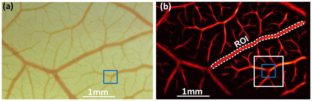
Quantitative analysis for super-resolution ultrasound microvessel imaging (SR-UMI). (a) Microscopic image of the chorioallantoic membrane model, and (b) the same region as an SR-UMI vessel density map. The target patch, indicated by the blue box in (a), traversed the search window, indicated by the white box in (b),and the maximum cross correlation coefficient was recorded to quantify the local similarity between the two images. The target patch and the search window then traversed the entire image to quantify the overall similarity of SR-UMI to the microscopic image.

5). Quantitative analysis on vessel morphology with decreased imaging frame rate:

We acquired the ultrasound data at 500 Hz and down-sampled the data by different ratios to simulate different imaging scenarios with reduced MBs by virtually lowering the imaging frame rate (FR). For example, ultrasound images with an FR of 250 Hz were obtained by keeping one ultrasound frame out of every two consecutive frames; those with an FR of 100 Hz were obtained by keeping one out of every five frames. In practice, decreased MB detection could be caused by a reduced MB concentration, a low imaging SNR, a decreased imaging FR, and/or a decreased accumulation time. Compared to the total detected MB number with an FR of 500 Hz, the MB number decreases by 58.03% and 85.96% with an FR drop to 250 Hz and 100 Hz, respectively. To keep MB pairing in a relatively consistent period of time, an MB has to be paired in 10 consecutive frames for a 500 Hz imaging rate, 5 for 250 Hz, and 3 for 10 Hz.

Binary vasculature morphology was first obtained from an SR-UMI image using Otsu’s thresholding method with 256-bin histogram [28] (MATLAB function imbinarize.m). An ROI was selected from a blood vessel, as illustrated by the white dashed lines in Fig. 3(b). The percentage of microvessel filling in the selected ROI was calculated as:

$$\text{VF}=\frac{N_{marked}}{N_{total}}\times 100\%,$$ (9)

where N_total denotes the total pixel number inside the ROI, while N_marked is the number of pixels marked in the binary SR-UMI image.

6). Quantitative analysis of SR-UMI contrast to noise ratio:

A contrast to noise ratio (CNR) comparison was conducted in a selected ROI mainly containing a blood vessel and an ROI mainly containing noise. The CNR was calculated as [29]:

$$\text{CNR}=\frac{\left|E_V-E_N\right|}{{\sigma }_N},$$ (10)

where E_V and E_N are the mean intensities of the selected vessel ROI (“V” areas in Fig. 9) and noise ROI (“N” areas in Fig. 9), respectively, while σ_N is the standard deviation of the noise ROI.

Fig. 9.

Contrast to noise ratio (CNR) comparison in the super-resolution ultrasound microvessel imaging (SR-UMI) on the rabbit kidney model. Vessel and noise regions of interest, indicated by “V” and “N”, respectively, are marked in each sub-figure. CNR of the SR-UMI without using any proposed processing (a), with using Kalman filtering (b), with using Kalman filtering and the two constraints (c), with using the proposed workflow including Kalman filtering, the two constraints, and with the adaptive interpolation (d) are 3.10, 4.88, 11.20, and 13.31, respectively.

B. Ex ovo CAM model

Fertilized chicken eggs were obtained from Hoover’s Hatchery (Rudd, IA) and stored in a heated (37°C), automatic-turning incubator until the fourth day of embryonic development. Ex ovo chicken embryo cultures were prepared by puncturing the eggshell with a rotary tool and transferring the egg contents into a plastic weight boat. Embryos were then transferred into a heated humidified incubator until ultrasound imaging on the 18th day of embryonic development. Approval from the Institutional Animal Care and Use Committee (IACUC) was not necessary to perform the chicken embryo-based experiments presented in this study.

A Verasonics Vantage ultrasound system (Verasonics Inc., Kirkland, WA) and a L35-16v high-frequency linear transducer array (Verasonics Inc., Kirkland, WA) with a center frequency of 25 MHz were used to provide plane-wave ultrasound transmission. Imaging was performed using 5 steering angles for plane-wave compounding (−4°, −2°, 0°, 2°, 4°), with each angle repeated 3 times to boost the SNR [30]. No special pulse sequencing technique, such as contrast pulse sequencing, amplitude modulation, or pulse inversion, etc. were used in this study. The receiving demodulation frequency was 25 MHz, as fundamental compounding plane imaging was adopted for MB detection. The post-compounding ultrasound FR was 500 Hz. The Vantage system uses an interleaved sampling scheme to sample a high frequency probe with an upper bandwidth limit above 25MHz. The samples from two successive transmit-receive acquisitions are combined, and the sampling points in the second acquisition are shifted by half of the A/D sampling period from those in the first. In this study, two acquisitions at a 62.5 MHz sample rate were combined to produce an effective sample rate of 125 MHz. Lumason suspension (Bracco Diagnostics Inc., Monroe Township, NJ), which was prepared with a 5x higher concentration than its original. All contrast-enhanced ultrasound imaging in the CAM model was performed using an intravenous injection of 70 μl Lumason suspension [31, 32]. A total of 21 datasets were collected with one bolus injection within 10 minutes, each containing 720 ensembles (data acquiring time duration was 1.44 seconds per dataset followed by a non-operation time of 20 seconds for data transfer and saving).

Microscopic images were acquired using a Nikon SMZ18 stereomicroscope (Nikon Corporation, Tokyo, Japan) at 4x magnification to provide the reference standard for ultrasound imaging. Images were digitized using an integrated Nikon DS-Ri2 digital camera (Nikon Corporation, Tokyo, Japan). Microscopic images were taken from the top of the weight boat containing the embryo. The ultrasound transducer was placed at the side of the weight boat to have a field of view (FOV) that included the CAM surface vessels. The microscopic imaging FOV was selected carefully according to the ultrasound images.

C. In vivo rabbit kidney model

The in vivo rabbit data was collected previously for a past study [33]. Here we reprocessed it and compared the reprocessing results with our previous results. The data was collected from a female New Zealand white rabbit. The experiment conformed to the policy of the IACUC at Mayo Clinic. The rabbit was anesthetized with ketamine (35.0 mg/kg) and xylazine (6.0 mg/kg). A Verasonics Vantage ultrasound system and a linear transducer array L11-4v (Verasonics Inc., Kirkland, WA) with a center frequency of 8.929 MHz were used for the rabbit model. A five-angle (−4°, −2°, 0°, 2°, 4°) plane-wave spatial compounding was used, with each angle repeated three times. The receiving demodulation frequency was also 8.929 MHz, as fundamental compounding plane imaging was adopted for MB detection. The effective post-compounding FR was 500 Hz. The right kidney of the rabbit was scanned freehand with the rabbit breathing freely. One bolus injection of 0.1 mL Optison (GE Healthcare, Milwaukee, WI, USA) suspension was administered through the marginal ear vein, followed by a 1 mL saline flush. In each second, 275 ensembles were collected within 0.55 seconds, followed by a non-operation time of 0.45 seconds (FR 500 Hz). A total of 15 datasets were continuously acquired in 15 seconds. The ultrasound FOV was carefully selected to contain only in-plane motion caused by breathing. Ultrasound acquisition started when the kidney was fully perfused with MBs.

III. Results

A. Kalman filtering smooths the MB trajectory and improves the precision of blood flow speed estimation

The movement of blood flow is either laminar or turbulent. Laminar flow is characterized by fluid particles following smooth paths in layers. The motion of the particles is orderly, with particles moving in straight lines parallel to the surface [34]. On the other hand, turbulent flow is characterized by chaotic changes in the movement trajectory [34]. However, the distorted and chaotic movement happens on a relatively macro scale. In this study, a p step trajectory was captured in 20-30 ms. For such a short duration, we assumed a smooth moving trajectory of MBs with moderate flow speed in a turbulent flow pattern. Figure 4 shows the microvessel density and flow speed maps obtained before and after using the linear interpolation-based processing [14] and the proposed Kalman filter-based processing methods. While similar performance was observed among different methods in the microvessel density maps (Fig. 4(a)–(c)), Kalman filtering produced much smoother flow speed maps (Fig. 4(f)) with low standard deviations (Fig. 4(g)). This is expected because MB locations and tracking contaminated by noisy MB signals typically result in an increased traveling distance, resulting in overestimation of MB flow speed. Figure 4(h) shows a typical 10-step MB trajectory (green dotted line) estimated from localizing the centroid of MB signals on 10 consecutive ultrasound frames (described in boxes 1-6 in Fig. 1). Several steps of this trajectory did not follow the direction of the vessel in which the MB was located. Figure 4(i)–(j) outlines the trajectories obtained from linear interpolation-based processing (white dotted line) and Kalman filtering (blue dotted line). It can be clearly seen that Kalman filtering produces the smoothest trajectory, most consistent with the morphology of the microvessel where the MB was detected. A small ROI was selected in Fig. 4(f) for the quantitative analysis in Fig. 4(g), where a more uniform flow speed was observed using the Kalman filter. In practice, a smaller standard deviation is more realistic considering the ROI selected is a very limited portion of the vessel; therefore, it should have a relatively consistent flow speed.

Fig. 4.

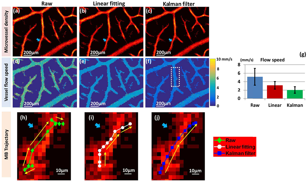
Comparison of microvessel density maps and flow speed maps of the chorioallantoic membrane surface vessel before and after linear interpolation-based processing and Kalman filter-based processing. The first column shows the original super-resolution ultrasound microvessel imaging (SR-UMI), obtained with the steps outlined in box 1-6 in Fig. 1. The second and third columns are SR-UMIs with further linear interpolation-based processing and Kalman filter-based processing, respectively. (a) – (c) Microvessel density maps. (d) – (f) Vessel flow speed maps, including a typical 10-step MB trajectory for each scenario. The blue arrows in (a)-(c) and (h)-(j) indicate the location of the selected vessel. (g) Bar plot of mean and standard deviation of vessel flow speed in the selected region of interest, indicated by the white dashed box in (f) for the three methods of flow speed measurement.

B. The constraints suppress MBs with high acceleration and/or an abrupt change of movement direction

Figure 5 shows the performance of the proposed MB movement constraints applied after the Kalman filter. With the microscopic image as the ground truth, one can clearly see that both the acceleration constraint and the direction constraint were effective at rejecting false MB locations (yellow and white arrows in Fig. 5(a)–(d)). Similar to the observation above, the improvement is more obvious from the microvessel flow speed maps shown in Fig. 5(e)–(h). Although a closer look at the arrow-indicated region of the microscopic image suggests the presence of capillaries, the high flow speed detected in this region, shown in Fig. 5(e), is less likely to be associated with capillary level vessels (i.e., flow speed in capillaries should be lower than the flow speed in nearby larger vessels). Therefore, these data points are more likely to be caused by false MB locations, which were effectively rejected by the proposed methods.

Fig. 5.

Comparison of microvessel density maps and vessel flow speed maps before and after applying microbubble movement constraints on the chorioallantoic membrane surface vessel. (a) – (d) Microvessel density maps. (e) - (h) Microvessel flow speed maps. (a) and (e) were obtained without using any constraint, (b) and (f) were with acceleration constraint only, (c) and (g) were with direction constraint only, (d) and (h) were with both constraints. (i) A microscopic image showing the same field of view as in (a)-(h).

Based on the measured microvessel flow speed, adaptive interpolation was then applied to recover the missing MB signals between two adjacent MB locations. For instance, MB signals were paired in 10 consecutive frames, and the maximum MB movement speed with the unit of pixels/frame in these 10 frames was used as the interpolation factor for this 10-step movement. The missing MB signals between two adjacent locations were then recovered, and the visual appearance of SR-UMI was substantially improved.

C. The proposed method improves the microvascular detection for SR-UMI

Similarity comparison between SR-UMI images and optical microscopy by means of the CCC was assessed with different MB accumulation times, as shown in Fig. 6(a). At any accumulation time, Kalman filtering combined with constraints and adaptive interpolation showed the highest similarity with the microscopic image.

Fig. 6.

Quantitative analysis on super-resolution ultrasound microvessel imaging (SR-UMI). (a) Normalized cross-correlation coefficients between the microscopic image and the SR-UMI images as a function of accumulation time. (b) Vessel filling percentage in the selected vessel region of interest (ROI, seen Fig. 3(b)) with the proposed method as a function of accumulation time with a frame rate (FR) of 100 Hz. (c) Vessel filling percentage in the selected vessel ROI for SR-UMI with FRs of 100 Hz and 500 Hz before and after processing. (d)-(f) and (g)-(i) are binary SR-UMI images before and after using the proposed methods for FR of 100 Hz, 250 Hz, and 500 Hz, respectively. One dataset (1.44 seconds accumulation) was used.

The vasculature morphology for imaging FRs of 100 Hz, 250 Hz, and 500 Hz before and after using the proposed methods are shown in Fig. 6(d)–(i). One dataset, equivalent to an accumulation time of 1.44s, was used for composing these images. As illustrated in Fig. 6(b), with the proposed method, the percentage of microvessel filling in the selected blood vessel with an imaging FR of 100 Hz gradually increased after each procedure. The highest increase in microvessel filling percentage was from 28.17% to 74.45% (when accumulating 3 datasets). Figure 6(c) compared the percentages of microvessel filling for FRs of 100 Hz and 500 Hz before and after processing. Before processing, the microvessel filling percentage of 100 Hz (blue) was lower than that of 500 Hz (red) at every accumulation time. However, after processing, the microvessel filling percentages of 100 Hz (yellow) and 500 Hz (purple) were comparable, demonstrating that the proposed method effectively improved blood vessel morphology acquired with low MB accumulation quantity, leading to an SR-UMI performance comparable to that acquired with a high MB number. Therefore, the proposed technique potentially benefits the imaging scenario with a reduced MB concentration, a low imaging SNR, a decreased imaging FR, and/or a decreased accumulation time.

D. SR-UMI for in vivo rabbit kidney blood vessels

Figure 7 (microvessel density maps) and Fig. 8 (vessel flow speed maps with movement speed and direction using a color wheel) show the SR-UMI results of an in vivo rabbit kidney. These results further demonstrate the effectiveness of the proposed Kalman filter-based method in facilitating more robust MB tracking and more precise vessel flow speed estimation. False MB localization and pairings led to a large number of MBs marked in gaps between microvessels and unreliable flow speed estimation, as illustrated in Fig. 7(a) and 8(a). With the use of Kalman filter-based tracking, MB movements were smoothened, which improved the precision of both blood flow speed and flow direction estimates. With the use of the MB movement constraints, false MB locations and pairings were rejected, and the performance of SR-UMI was further improved, as illustrated in Fig. 7(b) and 8(b).

Fig. 7.

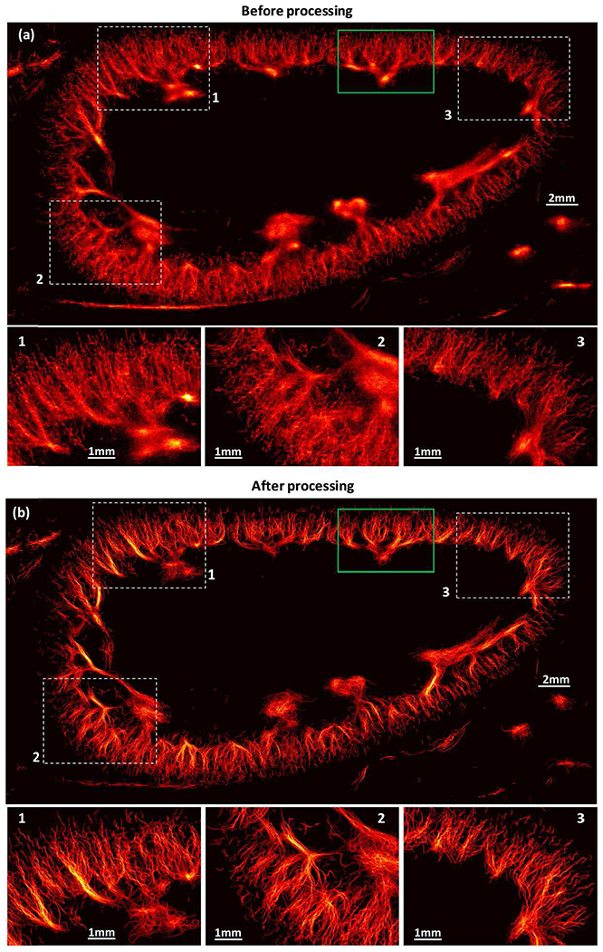
Vessel density maps of in vivo rabbit kidney in a free-breathing rabbit before (a) and after (b) using the proposed methods for super-resolution ultrasound microvessel imaging.

Fig. 8.

Vessel flow speed maps of in vivo rabbit kidney in a free-breathing rabbit before (a) and after (b) using the proposed methods for super-resolution ultrasound microvessel imaging.

An enlarged view of the ROI indicated by the green box in Fig. 7(a) is shown in Fig. 9. Rabbit kidney SR-UMIs presented show the comparison of images without using any of the proposed processing (Fig. 9(a)), with using the Kalman filter (Fig. 9(b)), with using the Kalman filter and the two constraints (Fig. 9(c)), and with using the entire proposed workflow (Kalman filter, constraint, and the adaptive interpolation; Fig. 9(d)). The CNR was increased from 3.10 to 13.31 with the use of the proposed method. One can easily see that the CNR was largely improved after using the acceleration and direction constraints, as the noise was suppressed effectively.

IV. Discussion

A Kalman filter-based MB tracking method was proposed in this study to improve the robustness of SR-UMI and the precision of blood flow speed estimation. The SR-UMI images acquired with CAM surface vessels exhibited improved similarity to the microscopic image, which was used as the ground truth. The percentage of microvessel filling in a selected vessel ROI increased from 28.17% to 74.45% after using the proposed methods. Thus, the proposed method greatly improved the depiction of vessel morphology, especially for the scenario with reduced number of MBs due to a low MB dose or limited imaging FR. This facilitates the use of more steer angles or complex acquisition schemes during ultrasound transmit-receive acquisitions, which further benefits the SNR for MB signal detection.

The Kalman filter was first adopted for MB aided ultrasound imaging in [8, 9], where the Kalman filter was one of many components in a large network of the algorithms “the modified Markov chain Monte Carlo data association (MCMCDA)” in [8] and “the simultaneous sparsity-based super-resolution tracking (3SAT)” in [9]. In contrast, here we did a specific study that uses Kalman filtering for MB tracking in the context of improving the performance of conventional ultrasound localization microscopy (ULM). Any research group or investigator using ULM could benefit from the findings of this study. The upstream processing techniques (the steps before Kalman filtering, shown in boxes 1-6 in Fig. 1) can be adjusted and customized according to the specific imaging application, instead of having to use the entire algorithm proposed by MCMCDA or 3SAT. In addition, one of the purposes of our study was to inpaint the super resolved vessel density map with a limited number of MBs. However, the improvement due to Kalman filtering on the vessel density map in Fig. 4(c) is not as obvious as its improvement on the blood flow speed map in Fig. 4(f) because Kalman filtering does not improve MB localization. Microbubble trajectories were smoothed following Kalman filtering, and the acceleration and direction constraints could distinguish and remove false MB trajectories while preserving real MB signals for inpainting, in accordance with blood flow kinematics. This leads to an improved performance on vessel density maps, as illustrated in the CNR comparison in Fig. 9.

The raw SR-UMI images without processing presented in Fig. 4(a), 4(d), 4(h), 6(d)–(f), 7(a), and 8(a) were generated with steps that included image registration, tissue clutter filter, de-noising, spatial interpolation (to the desired resolution), MB localization, and MB pairing in p consecutive frames, as illustrated in Fig. 1. These are considered upstream steps. The after-processing SR-UMI images were completed with add-on steps, including Kalman filtering, MB movement constraints, and adaptive interpolation steps. Similarly, the animal model, ultrasound frequency, de-noising technique, contrast agent type, etc., are considered upstream variables; these are also the same as the before- and after-processing SR-UMI for a given imaging application. The proposed Kalman-filter based data processing workflow is independent from the upstream variables and steps. No cross-model or cross-system comparison was conducted. Results generated from the two animal models showed improvements on imaging performance, demonstrating the applicability of the proposed method.

Compared to the rabbit kidney model, the imaging environment of the CAM model was very stable without tissue motion. Also, the blood flow speed in the chicken embryo model was relatively low. However, using a 2D imaging technique to track 3D movements is intrinsically a flawed approach that results in false MB localization and tracking, even in an ideal imaging environment. One can easily speculate this from the MB trajectory presented in Fig. 4(h), where the MB’s behavior was not compatible with the physiological and physical situation. Although this noise-containing MB localization has low impact on the microvessel density map (Fig. 4(a)), it seriously impacts the estimates for vessel flow speed (Fig. 4(d)).

We applied the two MB movement constraints directly on the paired MB signals without conducting Kalman filtering. As a result, a large number of MB signals were rejected due to distorted MB trajectories. In contrast, with the use of Kalman filtering, MB trajectory was smoothed, not only leading to a precise flow speed estimation (Fig. 1(f)), but also preserving more MB signals for more robust microvascular visualization, which is important for SR-UMI with a limited MB number. In comparison with previously reported studies [8, 9] which also employed Kalman filtering for ULM, we extended the benefit of Kalman filtering from only improving the flow speed estimation to also improving the performance of microvessel density mapping by introducing further MB trajectory quality control steps (the two constraints). One can see from Fig. 4 that the improvement on the microvessel morphology map via the Kalman filter is less obvious than its improvement on the blood flow map, since the Kalman filter does not remove false MB localizations or trajectories. However, with the smoothened MB trajectories, the two constraints could be applied, eliminating MB trajectories from false MB localization and pairing. As a result, the imaging CNR was improved due to the suppression of noise signal, as demonstrated in Fig. 9.

The flow speed map of the rabbit kidney vessel in Fig. 8(a) shows as a yellow-greenish color. This corresponds to an MB moving angle of zero in the color wheel, since the moving angle information at a given pixel is generated by averaging the moving angles of all MBs detected at this pixel. The detected MB moving angle was estimated in a range of [−π, π ]. When an MB location is contaminated by random noise, its moving angle also contains random disturbance, causing the accumulated and averaged moving direction on the final flow speed map back to zero. In contrast, the Kalman filter was able to smooth the trajectory and produce a more consistent movement direction, leading to an averaged-angle coherent with the angle of the vessel, as shown in Fig. 8(b).

Figure 10 shows the total marked MB points and MB trajectories before and after applying the constraints. An MB has to be persistently paired in consecutive p frames to be preserved as a valid MB signal. To keep an MB paired in a consistent period of time, it has to be paired in 10 consecutive frames for a 500 Hz imaging rate, 5 for 250 Hz, and 3 for 100 Hz. The total number of MBs preserved at 100 Hz, 250 Hz, and 500 Hz FRs are 95.82%, 88.57%, and 60.58%, respectively, after applying the constraints. The high preservation rate for the 100 Hz FR is caused by the low pairing persistent control used for 100 Hz (p = 3).

Fig. 10.

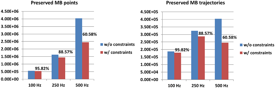
Preserved microbubble points (a) and trajectories (b) with and without applying the constraints at different tested frame rates.

The adaptive acceleration threshold used in Eq. (7) was based on the estimated MB speed, which is possibly biased by the inaccurate MB localization and pairing due to the residual noise and the inherent limitation of using a 2D imaging technique to track 3D MB movements. However, several steps in the processing chain (Fig. 1) were applied prior to the acceleration constraint to minimize noise and improve the accuracy of the MB speed/acceleration estimation. Figure 4(g) demonstrates that the accuracy of the estimated flow speed was substantially improved with the use of the Kalman filter. Although false MB localizations and pairings were still inevitable, validation from the in vivo and the ex ovo models supports the fidelity and accuracy of the MB tracking to a level satisfactory for threshold determination. In addition, selection of the adaptive acceleration threshold does not have to be the same as the one used in this study and can be determined based on a specific imaging application. Finally, a constant acceleration threshold might also work for some imaging applications. A constant threshold of 1000mm/s² (2mm/s change in 1/500 s) for the ex ovo CAM model led to an imaging performance similar to that with the adaptive acceleration threshold. However, a degraded imaging quality was observed for the in vivo rabbit kidney model with a constant acceleration threshold because of the relatively inconsistent blood flow speed in vessels at all levels.

The estimated MB movements in big vessels and at the junctions between big and small vessels are complicated due to the complex flow pattern in these structures. That factor, along with the inherent limitation of using 2D imaging to track 3D MB movements, results in unpredictable and various MB movement trajectories. Therefore, MBs were prone to be eliminated by the constraints at the aforementioned structures. Additional or more adaptive constraints may be possible to better accommodate various MB behaviors at these locations.

The thresholds of the acceleration and direction constraints for the CAM model and the rabbit kidney model were empirically derived in this study. The thresholds may need to be adjusted for different applications. For example, tumor vessels are more tortuous and tumor blood flow speed can be lower than in normal tissue [35], leading to larger MB turning angles and/or lower acceleration than that in normal tissue. As a result, the tolerance for MB direction and acceleration change should be adjusted accordingly when new constraints are adopted.

The adaptive interpolation was able to make up the missing MBs in between the detected ones, and therefore, better restore the vessel morphology when originally limited MB signal showed up in the vessel. From this perspective, the proposed method shortened the imaging time for SR-UMI. However, we want to be cautious about this statement, as the proposed method is based on the fact that MB trajectory is detected in the first place. In practice, peripheral blood vessels, especially at the capillary level, require a period of time to have an MB population that can be reliably detected. As reported in [36], the time necessary for vessels of different size to be completely reconstructed in ULM varied substantially. Reconstruction time increases dramatically for 30 μm and smaller vessels (> 10 min in their case), and is primarily dictated by hemodynamics.

Some capillaries observable in the microscopic image (Fig. 5(a)) could not be depicted with the current SR-UMI (Fig. 5(b) and 6(i)), even with the highest imaging FR (500 Hz) and longest accumulation time used in this study. In fact, it is well-known that MBs are not able to be detected in capillaries, especially for the CAM surface vessel, which is the lung of the chicken. Ferrara’s group reported that MB expansion was significantly reduced when MBs were constrained within small vessels due to low vessel compliance [37, 38], suggesting that MB echoes would be difficult to detect in such regions. De Jong et al. also observed a highly nonlinear response of phospholipid-coated MBs [39], suggesting that using a nonlinear mode may be better for tracking bubbles in capillaries. However, since the fundamental frequency used for the CAM model was high (25 MHz), it was challenging to implement nonlinear imaging techniques using second harmonics. Also, we did not deploy other nonlinear imaging techniques because of FR concerns. At 25 MHz, we already needed to sacrifice the imaging FR by a factor of 2 by using interleaved sampling for the Verasonics Vantage system. The use of nonlinear imaging sequences (e.g., AM, PIAM, etc.) requires multiple transmissions, further reducing imaging FR.

V. Conclusion

In summary, we implemented the Kalman filter in SR-UMI for robust MB tracking and more precise blood flow speed measurements. According to physiological behavior of MBs moving in blood vessels, two constraints were specifically developed to eliminate MBs with abrupt changes in movement acceleration and/or direction. Then, an adaptive interpolation approach was developed to inpaint the missing microvessel signals based on the estimated local blood flow speed, facilitating more robust depiction of microvasculature with a limited amount of MBs. Results on an ex ovo CAM model and a in vivo rabbit kidney model demonstrated improved imaging performance on both vessel density and flow speed maps. The percentage of microvessel filling increased from 28.17% to 74.45% in a selected blood vessel using the proposed methods when the total MB number was reduced by 85.96%. Similar SR-UMI performance was achieved using a reduced MB number when compared to using the original MB number. Based on the presented SR-UMI images and the quantitative results, the proposed method substantially improves the robustness of SR-UMI and is important for its clinical translation.

Biographies

Shanshan Tang received the B.S. degree in biomedical engineering from Xi’an Jiaotng University, Xi’an, China, in 2008, and the Ph.D. degree in biophysics from Xi’an Jiaotong University, Xi’an, China, in 2014. She is now with the Department of Radiology, Mayo Clinic College of Medicine, Rochester, Minnesota, USA. Her current research interests include ultrasound super resolution imaging and ultrasound microvessel imaging.

Pengfei Song (IEEE/S’09/M’14/SM’19) received the B.Eng. degree in Biomedical Engineering from the Huazhong University of Science and Technology, Wuhan, China, in 2008; the M.S. degree in Biological Systems Engineering from the University of Nebraska-Lincoln, Lincoln, NE, in 2010; and the Ph.D. degree in Biomedical Sciences-Biomedical Engineering from the Mayo Graduate School, Mayo Clinic College of Medicine, Rochester, MN, in 2014. He is currently an Assistant Professor in the Department of Electrical and Computer Engineering, and the Beckman Institute for Advanced Science and Technology at the University of Illinois at Urbana-Champaign, Urbana, IL. His current research interests are super-resolution ultrasound microvessel imaging, ultrafast 3D imaging, deep learning, functional ultrasound, and ultrasound shear wave elastography. Dr. Song is a senior member of IEEE, full member of ASA, and member of AIUM and Sigma Xi.

Joshua D. Trzasko (IEEE/M’99/SM’2014) received the B.S. degree in Electrical and Computer Engineering in 2003 from Cornell University and the Ph.D. degree in Biomedical Engineering from Mayo Graduate School in 2009. He is currently a Senior Associate Consultant in the Division of Medical Physics and Assistant Professor of Radiology and Biomedical Engineering at Mayo Clinic. Dr. Trzasko’s research focuses on the development and application of statistical signal processing methods for medical imaging, including: quantitative imaging, artifact correction, and limited data reconstruction in magnetic resonance imaging (MRI); radiation dose reduction in x-ray computed tomography (CT); and ultrasound (US) microvasculature imaging.

Matthew Lowerison received the Ph.D degree in Medical Biophysics from the University of Western Ontario, London, Ontario, Canada in 2017. He is now with the Department of Electrical and Computer Engineering and the Beckman Institute for Advanced Science and Technology at the University of Illinois at Urbana-Champaign, Urbana, IL. His current research interests include ultrasound microvessel imaging, super-resolution ultrasound localization microscopy, and ultrasonic characterization of tumor microenvironments.

Chengwu Huang received the B.S. degree in biomedical engineering from Beihang University, Beijing, China, in 2012, and the Ph.D. degree from the Department of Biomedical Engineering at Tsinghua University, Beijing, China, in 2017. He is now with the Department of Radiology, Mayo Clinic College of Medicine, Rochester, Minnesota, USA. His current research interests include ultrasound microvessel imaging and ultrasound elastogrpahy.

Ping Gong received the B.Sc degree from Tianjin University, China, majoring Biomedical Engineering in 2010. She completed her M.Sc. degree in the Department of Electrical and Computer Engineering at Lakehead University, Canada in 2012 and Ph.D. in Biomedical Physics, Ryerson University in 2016. She is now with the Department of Radiology, Mayo Clinic College of Medicine, Rochester, Minnesota, USA. Her research focuses on developing ultrasound transmission and beamforming algorithms to improve ultrasound image quality.

U-Wai Lok U-Wai Lok received the B.S. and M.S. degree in electrical engineering from the National Chiao Tung University, Hsinchu, Taiwan, respectively in 2006 and 2008. Then, he joined the Sunplus technology, Hsinchu Science Park, Taiwan, as a member of the electrical engineer, where his work was focusing on signal processing. He received the Ph.D. degree in the Institute of Biomedical Electronics and Bioinformatics, National Taiwan University in 2017. He is now with the Department of Radiology, Mayo Clinic College of Medicine, Rochester, Minnesota, USA. His current research interests include ultrasonic microvessel imaging and super-resolution ultrasound microvessel imaging.

Armando Manduca (SM’89) received the B.S. degree in mathematics from the University of Connecticut, Mansfield, CT, USA, in 1974, and the Ph.D. degree in astronomy from the University of Maryland, College Park, MD, USA, in 1980. He is currently a Professor of Biomedical Engineering and Radiology, and the Chair of the Division of Biomathematics and Translational Engineering with Mayo Clinic, Rochester, MN, USA. His research interests include the development of algorithms for the analysis of MR and ultrasound elastography data, image denoising for CT data to reduce radiation dose, and ultrasound microvessel imaging.

Shigao Chen (IEEE/M’02) received the B.S. and M.S. degrees in biomedical engineering from Tsinghua University, China, in 1995 and 1997, respectively, and the Ph.D. degree in biomedical imaging from the Mayo Graduate School, Rochester, MN, in 2002. He is currently a Professor of the Mayo Clinic College of Medicine. His research interest is noninvasive quantification of the viscoelastic properties of soft tissue using ultrasound, and ultrasound microvessel imaging.

References

- [1].Errico C et al. , “Ultrafast ultrasound localization microscopy for deep super-resolution vascular imaging,” Nature, vol. 527, pp. 499–502, Nov. 2015. [DOI] [PubMed] [Google Scholar]
- [2].Christensen-Jeffries K et al. , “In Vivo Acoustic Super-Resolution and Super-Resolved Velocity Mapping Using Microbubbles,” IEEE Trans. Med. Imaging, vol. 34, no. 2, pp. 433–440, Feb. 2015. [DOI] [PubMed] [Google Scholar]
- [3].Ackermann D and Schmitz G, “Detection and Tracking of Multiple Microbubbles in Ultrasound B-Mode Images,” IEEE Trans. Ultrason. Ferroelectr. Freq. Control, vol. 63, no. 1, pp. 72–82, Jan. 2016. [DOI] [PubMed] [Google Scholar]
- [4].Viessmann OM et al. , “Acoustic super-resolution with ultrasound and microbubbles,” Phys. Med. Biol, vol. 58, no. 18, pp. 6447–6458, 2013. [DOI] [PubMed] [Google Scholar]
- [5].Lin F et al. , “3-D Ultrasound Localization Microscopy for Identifying Microvascular Morphology Features of Tumor Angiogenesis at a Resolution Beyond the Diffraction Limit of Conventional Ultrasound,” Theranostics, vol. 7, no. 1, pp. 196–204, Jan. 2017. [DOI] [PMC free article] [PubMed] [Google Scholar]
- [6].Bar-Zion A et al. , “Fast Vascular Ultrasound Imaging With Enhanced Spatial Resolution and Background Rejection,” IEEE Trans. Med. Imaging, vol. 36, no. 1, pp. 169–180, Jan. 2017. [DOI] [PubMed] [Google Scholar]
- [7].Hansen KB et al. , “Robust microbubble tracking for super resolution imaging in ultrasound,” 2016 IEEE International Ultrasonics Symposium (IUS), Tours, 2016, pp. 1–4. [Google Scholar]
- [8].Ackermann D, and Schmitz G. “Detection and tracking of multiple microbubbles in ultrasound B-mode images,” IEEE Trans. Ultrason. Ferroelectr. Freq. Control, vol. 63, no. 1, pp. 72–82, Jan. 2016. [DOI] [PubMed] [Google Scholar]
- [9].Solomon Oren, et al. , “Exploiting flow dynamics for super-resolution in contrast-enhanced ultrasound,” IEEE Trans. Ultrason. Ferroelectr. Freq. Control, vol. 66, no. 10, pp. 1573–1586, Oct. 2019. [DOI] [PubMed] [Google Scholar]
- [10].Opacic T et al. , “Motion model ultrasound localization microscopy for preclinical and clinical multiparametric tumor characterization,” Nat. Commun, vol. 9, pp. 1527, Apr. 2018. [DOI] [PMC free article] [PubMed] [Google Scholar]
- [11].Ghosh D et al. , “Monitoring early tumor response to vascular targeted therapy using super-resolution ultrasound imaging,” 2017 IEEE International Ultrasonics Symposium (IUS), Washington, DC, 2017, pp. 1–4. [Google Scholar]
- [12].Lin F, Rojas JD, and Dayton PA, “Super resolution contrast ultrasound imaging: Analysis of imaging resolution and application to imaging tumor angiogenesis,” 2016 IEEE International Ultrasonics Symposium (IUS), Tours, 2016, pp. 1–4. [Google Scholar]
- [13].Hingot V et al. , “Subwavelength motion-correction for ultrafast ultrasound localization microscopy,” Ultrasonics, vol. 77, pp. 17–21, May 2017. [DOI] [PubMed] [Google Scholar]
- [14].Song P et al. , “Improved Super-Resolution Ultrasound Microvessel Imaging With Spatiotemporal Nonlocal Means Filtering and Bipartite Graph-Based Microbubble Tracking,” IEEE Trans. Ultrason. Ferroelectr. Freq. Control, vol. 65, no. 2, pp. 149–167, Feb. 2018. [DOI] [PMC free article] [PubMed] [Google Scholar]
- [15].Song P et al. , “On the Effects of Spatial Sampling Quantization in Super-Resolution Ultrasound Microvessel Imaging,” IEEE Trans. Ultrason. Ferroelectr. Freq. Control, vol. 65, no. 12, pp. 2264–2276, Dec. 2018. [DOI] [PMC free article] [PubMed] [Google Scholar]
- [16].Heiles B et al. , “Volumetric ultrafast ultrasound localization microscopy using a 32×32 matrix array,” 2017 IEEE International Ultrasonics Symposium (IUS), Washington, DC, 2017, pp. 1–1. [Google Scholar]
- [17].Hingot V et al. , “Microvascular flow dictates the compromise between spatial resolution and acquisition time in Ultrasound Localization Microscopy,” Sci. Rep, vol. 9, p. 2456, Feb. 2019. [DOI] [PMC free article] [PubMed] [Google Scholar]
- [18].Harput S et al. , “3-D Super-Resolution Ultrasound Imaging With a 2-D Sparse Array”, IEEE Trans. Ultrason. Ferroelectr. Freq. Control, vol. 67, no. 2, pp. 269–277, Feb. 2020. [DOI] [PMC free article] [PubMed] [Google Scholar]
- [19].Heiles B et al. , “Ultrafast 3D Ultrasound Localization Microscopy Using a 32 × 32 Matrix Array,” IEEE Trans. Med. Imaging, vol. 38, no. 9, pp. 2005–2015, Sep., 2019. [DOI] [PubMed] [Google Scholar]
- [20].Rabut C et al. , “4D functional ultrasound imaging of whole-brain activity in rodents,” Nat. Methods, vol. 16, pp. 994–997, Oct. 2019. [DOI] [PMC free article] [PubMed] [Google Scholar]
- [21].Musoff H and Zarchan P, Fundamentals of Kalman Filtering: A Practical Approach, VA, Reston:AIAA, vol. 208, 2005. [Google Scholar]
- [22].Song P et al. , “Functional Ultrasound Imaging of Spinal Cord Hemodynamic Responses to Epidural Electrical Stimulation: A Feasibility Study,” Front. Neurol, vol. 26, pp. 279, Mar. 2019. [DOI] [PMC free article] [PubMed] [Google Scholar]
- [23].Foroosh H, Zerubia JB, and Berthod M, “Extension of phase correlation to subpixel registration,” IEEE Trans. Image Process, vol. 11, no. 3, pp. 188–200, Mar. 2002. [DOI] [PubMed] [Google Scholar]
- [24].Demene C et al. , “Spatiotemporal Clutter Filtering of Ultrafast Ultrasound Data Highly Increases Doppler and fUltrasound Sensitivity,” IEEE Trans. Med. Imaging, vol. 34, no. 11, pp. 2271–2285, Nov. 2015. [DOI] [PubMed] [Google Scholar]
- [25].Gomez-Gil J et al. , “A Kalman filter implementation for precision improvement in low-cost GPS positioning of tractors,” Sensors, vol. 13, no. 11, pp. 15307–15323, 2013. [DOI] [PMC free article] [PubMed] [Google Scholar]
- [26].Kalman RE, “A New Approach to Linear Filtering and Prediction Problems,” J. Basic Eng, vol. 82, no. 1, pp. 35–45, Mar. 1960. [Google Scholar]
- [27].Huber PJ, “Robust statistics: A review,” Ann. Math. Statist, vol. 43, no. 4, pp. 1041–1067, 1972. [Google Scholar]
- [28].Otsu N, “A Threshold Selection Method from Gray-Level Histograms,” IEEE Trans. Syst. Man Cybern, vol. 9, no. 1, pp. 62–66, Jan. 1979. [Google Scholar]
- [29].Demene C et al. , “Spatiotemporal Clutter Filtering of Ultrafast Ultrasound Data Highly Increases Doppler and fUltrasound Sensitivity,” IEEE Trans. Med. Imaging, vol.34, no. 11, pp. 2271–2285, Nov. 2015. [DOI] [PubMed] [Google Scholar]
- [30].Urban A et al. , “Real-time imaging of brain activity in freely moving rats using functional ultrasound,” Nat. Methods, vol. 12, no. 9, pp. 873, Sep. 2015. [DOI] [PubMed] [Google Scholar]
- [31].Diehl KH et al. , “A good practice guide to the administration of substances and removal of blood, including routes and volumes,” J. Appl. Toxicol, vol. 21, no. 1, pp. 15–23, Feb. 2001. [DOI] [PubMed] [Google Scholar]
- [32].Kind C, “The development of the circulating blood volume of the chick embryo,” Anat. Embryol, vol. 147, no. 2, pp. 127–132, Jan. 1975. [DOI] [PubMed] [Google Scholar]
- [33].Song P et al. , “Improved Super-Resolution Ultrasound Microvessel Imaging With Spatiotemporal Nonlocal Means Filtering and Bipartite Graph-Based Microbubble Tracking,” IEEE Trans. Ultrason. Ferroelectr. Freq. Control, vol. 65, no. 2, pp. 149–167, Feb. 2018. [DOI] [PMC free article] [PubMed] [Google Scholar]
- [34].Sleigh PA and Noakes CJ. CIVE 1400: An Introduction to Fluid Mechanics. www.efm.leeds.ac.uk/CIVE/fluidslevel1.
- [35].Fukumura D et al. , “Tumor microvasculature and microenvironment: Novel insights through intravital imaging in pre-clinical models,” Microcirculation, vol. 7, no. 3, pp. 206–225, Apr. 2010. [DOI] [PMC free article] [PubMed] [Google Scholar]
- [36].Hingot V et al. , “Microvascular flow dictates the compromise between spatial resolution and acquisition time in Ultrasound Localization Microscopy,” Sci. Rep, vol. 9, pp. 2456, Feb. 2019. [DOI] [PMC free article] [PubMed] [Google Scholar]
- [37].Caskey CF, “Direct observations of ultrasound microbubble contrast agent interaction with the microvessel wall,”, J Acoust. Soc. Am, vol. 122, no. 2, pp. 1191–200, Aug. 2007. [DOI] [PubMed] [Google Scholar]
- [38].Foiret J et al. , “Ultrasound localization microscopy to image and assess microvasculature in a rat kidney,” Sci. Rep, vol. 7, no. 1, p. 13662, Oct. 20 2017. [DOI] [PMC free article] [PubMed] [Google Scholar]
- [39].de Jong N et al. , ““Compression-only” behavior of phospholipid-coated contrast bubbles,” Ultrasound Med. Biol, vol. 33, no. 4, pp. 653–6, Apr. 2007 [DOI] [PubMed] [Google Scholar]