

Abstract
Dynamic 18F-FDG PET with tracer kinetic modeling has the potential to noninvasively evaluate human liver inflammation using the FDG blood-to-tissue transport rate K1. Accurate kinetic modeling of dynamic liver PET data and K1 quantification requires the knowledge of dual-blood input function from the hepatic artery and portal vein. While the arterial input function can be derived from the aortic region on dynamic PET images, it is difficult to extract the portal vein input function accurately from PET images. The optimization-derived dual-input kinetic modeling approach has been proposed to overcome this problem by jointly estimating the portal vein input function and FDG tracer kinetics from time activity curve fitting. In this paper, we further characterize the model properties by analyzing the structural identifiability of the model parameters using the Laplace transform and practical identifiability using computer simulation based on fourteen patient datasets. The theoretical analysis has indicated that all the kinetic parameters of the dual-input kinetic model are structurally identifiable, though subject to local solutions. The computer simulation results have shown that FDG K1 can be estimated reliably in the whole-liver region of interest with reasonable bias, standard deviation, and high correlation between estimated and original values, indicating of practical identifiability of K1. The result has also demonstrated the correlation between K1 and histological liver inflammation scores is reliable. FDG K1 quantification by the optimization-derived dual-input kinetic model is promising for assessing liver inflammation.
1. Introduction
Nonalcoholic steatohepatitis (NASH) is a progressive nonalcoholic fatty liver disease (NAFLD) affecting approximately 5–10 million patients in the United States [Michelotti et al., 2013, Musso et al., 2011]. The hallmark of NASH is hepatic inflammation and injury in the setting of hepatic steatosis [Wree et al., 2013]. Clinical assessment of liver inflammation can only be made by invasive liver biopsy [Lee and Park, 2014]. There is currently no effective noninvasive imaging method in the clinic. PET imaging of translocator protein (TSPO) has shown some promise in small-animal studies [Xie et al, 2012]. Its translation and adoption as a clinical tool, however, is likely to take time. On the other hand, 18F-fluorodeoxyglucose positron emission tomography (FDG-PET) is widely accessible in clinics. While static FDG-PET imaging provides information mainly related to hepatic steatosis [Keramida et al, 2014a, Keramida et al, 2014b] and does not show a potential for measuring liver inflammation [Wang et al., 2018], dynamic FDG-PET with improved kinetic modeling has been demonstrated to be promising for non-invasively assessing liver inflammation by quantifying the FDG blood-to-tissue transport rate K1 [Wang et al., 2017, Sarkar et al., 2017, Wang et al., 2018, Sarkar et al., 2019]. Because the liver receives dual blood supplies from the hepatic artery and portal vein [Keiding, 2012], accurate liver PET kinetic modeling and quantification of K1 require the knowledge of dual-blood input function (DBIF) [Wang et al., 2018, Brix et al., 2001, Munk et al., 2001]. Although the arterial input function can be derived from the aortic region on dynamic PET images, it can be difficult to extract the portal vein input function from PET images. The limited spatial resolution of PET and small anatomic size of the portal vein can result in serious partial volume effects and high noise in the image-derived input function [Mourik et al., 2008].
Traditional single-input kinetic modeling neglects the difference between the hepatic artery input function and portal vein input function, resulting in inaccuracy in kinetic parameter estimation [Brix et al., 2001, Munk et al., 2001]. Existing population-based DBIF approaches [Brix et al., 2001, Munk et al., 2001, Winterdahl et al., 2011] use the model parameters pre-determined by population means that were commonly derived using arterial blood sampling in animal studies, which however can become ineffective in human studies. Modified models ([Kudomi et al., 2009, Garbarino et al., 2015]) have been proposed but still have certain limitations, for example requiring extraction of multiple different liver time activity curves (TACs) or an additional gut TAC, which may present challenges in clinical applications. In contrast, the optimization-derived DBIF model [Wang et al., 2018] employs mathematical optimization to jointly estimate the parameters of DBIF and liver FDG kinetics. It directly utilizes image-derived arterial input function, requires no invasive arterial blood sampling or additional ROI operations, and is more adaptive to individual patients. With the improved kinetic modeling, the FDG blood-to-liver transport rate K1 was statistically associated with histopathologic grades of liver inflammation, while K1 by the traditional single-blood input function (SBIF) model and population-based DBIF model did not show a statistical significance [Wang et al., 2018].
Identifiability analysis is crucial for examining the stability of a kinetic model [Gunn, 1996, Mankoff et al., 2006, Delbary et al., 2016]. It characterizes whether or not the unknown parameters of a specified model can be uniquely determined from noise-free data (i.e., structural identifiability [Bellman and Astrom, 1970, Anderson, 1983]) and how reliably these parameters can be estimated from noisy measurements (i.e., practical identifiability [Miao et al., 2008, Miao et al., 2011]). Depending on the condition under which the mapping from the parameter space to the input/output space is one-to-one, there is global structural identifiability (one-to-one mapping is valid in the whole parameter space) and there is local structural identifiability (one-to-one mapping is valid locally in the parameter space). Note that even if a parameter is structurally identifiable, it may not be estimated with adequate accuracy from real measurements. Among different methods for identifiability analysis [Miao et al., 2011], the Laplace transform [Bellman and Astrom, 1970] is frequently used for structural identifiability analysis, and computer simulation based on Monte Carlo sampling is the most effective method for analyzing practical identifiability [Miao et al., 2008].
In dynamic PET, most of the popular kinetic models follow the first-order ordinary differential equations with linear parameters and are commonly structurally identifiable. Hence, previous identifiability studies in dynamic PET focused on practical identifiability analysis [El Fakhri et al., 2009, Mankoff et al., 1998, Muzi et al., 2006, Doot et al., 2010, Muzi et al., 2005]. For dual-input kinetic modeling, the optimization-derived DBIF model contains two additional parameters when compared with traditional SBIF and population-based DBIF model. While the new model has improved the practical correlation of FDG K1 with histology, the increased number of free parameters may potentially increase variance in kinetic parameter estimation, but little is known so far on the quantitative aspects of the modeling.
In this paper, we conduct a theoretical analysis using the Laplace transform to assess the structural identifiability and conduct a computer simulation to evaluate the practical identifiability using patient data of liver inflammation. The results from this study can be used to indicate the quantification accuracy and precision of model parameters and provide guidance for further improving kinetic modeling of dynamic liver PET data.
2. Structural identifiability analysis using the Laplace transform
2.1. Compartmental modeling by differential equations
Most compartmental models in dynamic PET imaging can be described by the following first-order ordinary differential equations:
| (1) |
| (2) |
| (3) |
where t is time; c(t) = [c1(t), c2(t), …, cn(t)]T is the system states which are assumed to be zero at initial time, where ci represents the time activity of the i-th compartment and n is the number of tissue compartments; u(t) is the system input, often representing the blood input function in dynamic PET; CT(t) is the system output, i.e., the measured time activity curve (TAC) by PET; A is a n by n matrix, b is a n by 1 vector, w is a n by 1 vector and v is a scalar vector. A, b, w and v are composed of the kinetic parameters θ = (θ1, θ2, …, θm) to be determined.
For a commonly used 3-compartment model (Fig. 1) such as for dynamic FDG-PET imaging, we have
| (4) |
| (5) |
| (6) |
| (7) |
| (8) |
| (9) |
where Cp(t) is the plasma input function; Cf(t) and Cm(t) are the concentration in the free FDG and metabolized FDG compartments, respectively. The superscript “T ” denotes matrix or vector transpose. θ = [vb, K1, k2, k3, k4] with K1, k2, k3, k4 denoting the rate constants of FDG transport among compartments. vb denotes the fractional blood volume.
Figure 1.
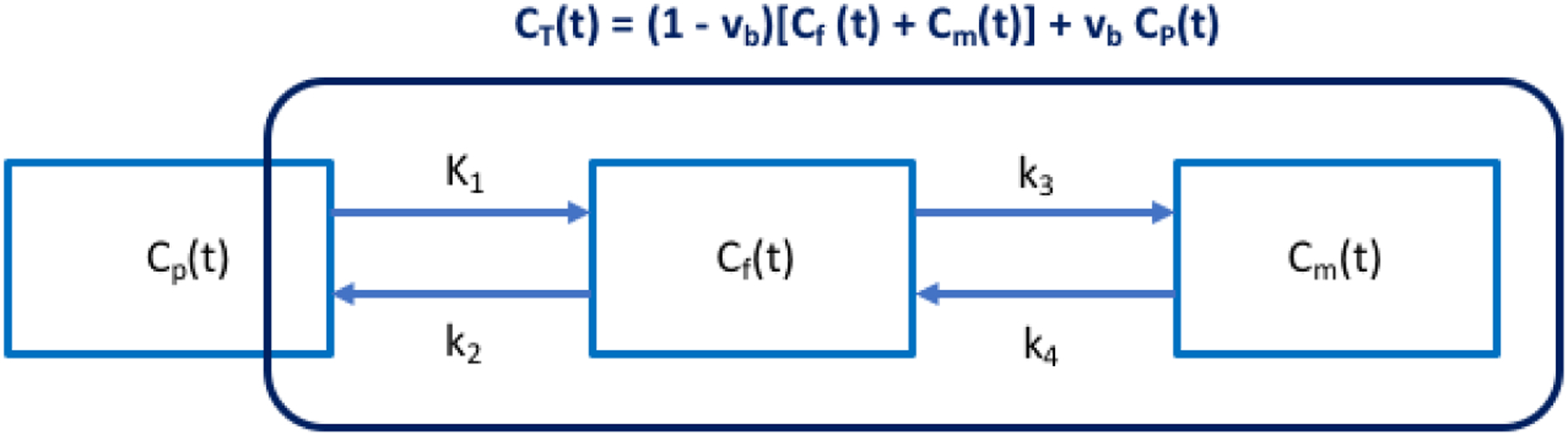
Three-compartment (Cp(t), Cf(t), Cm(t)) model with single-blood input function (SBIF). CT(t) denotes the total activity that can be measured by PET.
The optimization-derived DBIF model [Wang et al., 2018] for analyzing dynamic liver PET data is shown in Fig. 2 and can be described using the following expressions:
| (10) |
| (11) |
| (12) |
| (13) |
| (14) |
| (15) |
where CA(t) denotes the blood input function extracted from the hepatic artery; CPV(t) is the portal vein input function; ka is the rate constant with which FDG flows through the gastrointestinal system. fA is the fraction of hepatic artery contribution to the overall liver blood flow. The parameters to be determined are θ = [vb, K1, k2, k3, k4, ka, fA]T.
Figure 2.
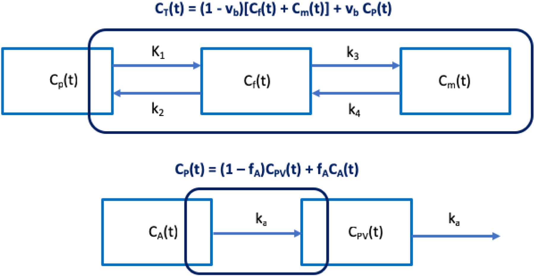
Optimization-derived dual-blood input function (DBIF) model. The FDG kinetic parameters (vb, K1, k2, k3, k4) and dual-input parameters (fA, ka) are jointly estimated by time activity curve fitting.
2.2. Laplace transform for structural identifiability analysis
The Laplace transform method is a popular method in the field of system theory for analyzing differential equations [Oppenheim et al., 1996, Tsien, 1954]. After the transform, the time derivative ∂/∂t becomes a multiplication of frequency s, thus simplifying the mathematical analysis. Taking the Laplace transform of equations (1) – (2) and making use of equation (3), one has
| (16) |
| (17) |
Where
| (18) |
represents the Laplace transform of any function f in the time domain.
The system input-output relation can then be expressed as
| (19) |
where Φ(s) is called the transfer function in the frequency domain,
| (20) |
with I denoting the identity matrix. Φ(s) can be further expressed as a fractional function
| (21) |
where both the numerator N(s) and denominator D(s) are a polynomial of the frequency s:
| (22) |
| (23) |
with r being the highest order of the polynomials of s. Ni is the coefficient of order i in N(s) and Di is the coefficient of order i in D(s). αi(θ) and βi(θ) describe the theoretical model of Ni and Di with respect to θ, respectively.
The structural identifiability analysis examines if the unknown parameter set θ can be uniquely determined from following the equation set:
| (24) |
| (25) |
for i from 0 to r. If there are arbitrary solutions for the equations, the model structure is non-identifiable. If the equations have a unique solution for any admissible input and in the whole parameter space, the model structure is called globally identifiable. If the solution only holds unique for a neighborhood of some points θ* in the parameter space, the structure is then locally identifiable. The single-input compartmental model for dynamic FDG-PET is globally identifiable [Gunn, 1996]. A brief proof is provided in the Appendix for the reader convenience.
2.3. Structural identifiability of dual-input kinetic modeling
For the optimziation-derived DBIF model, based on the derivations detailed in the Appendix, we can derive
| (26) |
which is a cubic equation of ka. In the real parameter space, the number of roots for ka is at least 1 and at most 3.
Similarly, for fA we have,
| (27) |
which is also a cubic equation when ka is fixed. The number of roots for fA with given ka in the non-negative parameter space is at least 1 and at most 3.
These results indicate that ka and fA are not globally identifiable because they may have multiple solutions. However, given there is at least one nonnegative root for ka and fA, they are locally identifiable. In practice, this requires a proper definition of initial estimates, lower and upper bounds for the parameters. Once ka and fA are determined, K1, k2, k3, k4 can then be determined respectively.
3. Practical identifiability analysis using computer simulation
3.1. Computer simulation
3.1.1. Overall description
The process of the computer simulation is described in figure 3. For each simulation, the nominal kinetic parameters θ0 and the input function CA(t) were extracted from one of the human patient datasets and used to generate the noise-free liver tissue time activity curves (TAC). Independently and identically distributed noise was then added to the noise-free TAC using random sampling, following a defined time-varying Gaussian noise model to generated N = 1000 realizations of noisy tissue TAC. We then fit the noisy liver tissue TACs and estimate the kinetic parameters of the optimization-derived DBIF kinetic model using nonlinear least-square fitting with the Levenberg-Marquardt algorithm described in our previous work [Wang et al., 2018]. Normalized bias, standard deviation (SD) and root mean square error (RMSE) were calculated to assess the statistical properties of each kinetic parameter estimation. This same simulation was done for multiple patient data sets.
Figure 3.
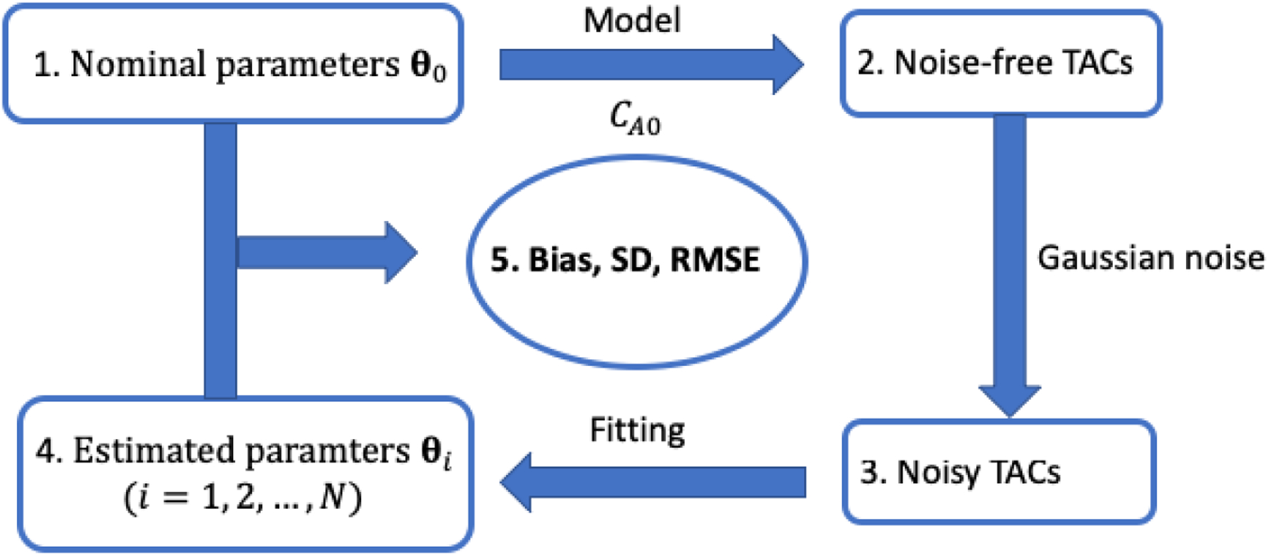
Flowchart of the practical identifiability analysis using computer simulation.
In addition to the kinetic parameters directly estimated by the model, the FDG net influx rate Ki = K1k3/(k2 + k3) was also evaluated.
3.1.2. Human liver FDG kinetics and histological data
Fourteen patients with NAFLD were included in this study to provide nominal kinetic parameters [Wang et al., 2018]. These patients had a liver biopsy as a part of routine clinical care or for enrollment in clinical trials. Liver biopsies were scored according to the nonalcoholic steatohepatitis clinical research network (NASH-CRN) criteria. An overall liver inflammation score (range 0–5) is obtained by combining the scores of lobular inflammation and ballooning degeneration (hepatocyte injury) as both reflect the inflammatory status in the total NAFLD activity [Sarkar et al., 2019]. Dynamic PET studies were performed using the GE Discovery 690 PET/CT scanner (axial field-of-view: 16 cm) at the UC Davis Medical Center. Each patient was injected with 10 mCi 18F-FDG. One-hour dynamic PET scanning was performed for a single bed position with the liver centered in the scanner field-of-view. A transmission CT scan was performed at the end of PET scan for attenuation correction. Dynamic PET data were reconstructed into 49 time frames (30×10s, 10×60s, and 9×300s) using the vendor software with the standard ordered subsets expectation maximization algorithm with 2 iterations and 32 subsets.
Eight spherical regions of interest (ROI), each with 25 mm in diameter, were placed on eight segments of the liver excluding the caudate lobe and avoiding any major blood vessels. An illustration is shown in Figure 4. A TAC was extracted from each liver-segment ROI. The average of these TACs was used to represent the tissue TAC in the whole-liver region. An additional volumetric ROI was placed in the descending aorta region to extract image-derived aortic input function. The optimization-derived DBIF model was used to derive the regional liver FDG kinetics at both the whole-liver ROI level and liver-segment ROI level. Hence there are a total 14 whole-liver FDG kinetic parameter sets and 112 liver-segment kinetic parameter sets from the 14 patient scans.
Figure 4.
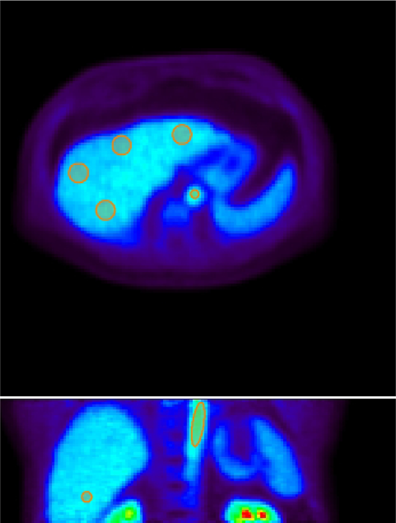
Illustration of volumetric ROIs in the liver segments and aorta in 2D planes. Top: a transverse plane showing the aortic ROI and four of eight spherical liver ROIs; Bottom: a coronal plane showing the aortic ROI and one of eight spherical liver ROIs. ROIs are overlayed on the PET image of one-hour duration. All the spherical liver ROIs are of 25 mm in diameter.
3.1.3. Noise model of TACs
The reconstructed time activity in the frame m, cm, can be approximately modeled by an i.i.d. Gaussian distribution [Wu and Carson, 2002, Carson et al., 1993],
| (28) |
where denotes the noise-free TAC and Sc is a scaling factor adjusting the amplitude of the unscaled standard deviation (SD) δm,
| (29) |
where tm is the mid-time of frame m, Δtm is the scan duration of the time frame m, and λ = ln 2/T1/2 is the decay constant of radiotracer with T1/2 (min) being the half-life. For 18F-FDG, T1/2 = 109.8 minutes.
Equivalently, the normalized residual difference follows a zero-mean Gaussian with the SD Sc:
| (30) |
From our patient study, we have a total 14 patients × 49 frames/patient = 686 samples for Δcm extracted at the whole-liver ROI level. The scale Sc can then be determined by approximating the histogram of Δcm using the Gaussian with the standard deviation Sc. Similarly, we have a total 686× 8 = 5488 samples to estimate Sc for the noise level at the liver-segment ROI level. Note that Eq. (30) is only used for deriving the global scaling factor of the noise level, not indicating the noise is uniform across frames. The actual noise of dynamic time frames, as modeled by Eq. (28), is time-varying and depends on the activity and scan duration of each frame.
3.2. Analysis methods
3.2.1. Sensitivity analysis
The sensitivity of a model TAC CT(t) with regard to a kinetic parameter k is defined by
| (31) |
and the normalized sensitivity is defined as
| (32) |
where k denotes the kth element of the kinetic parameter set θ and ∂CT(t)/∂θk denotes the partial derivative of CT(t) with respect to θk [Mankoff et al., 2006].
The sensitivity function illustrates how much the model TAC would change over time in response to a small change in the individual parameter θk. The larger the absolute value of the sensitivity is, the more sensitive the TAC would be to the change in the chosen parameter. While is used to evaluate the sensitivity over time for a specified parameter θk, the normalized sensitivity function is more appropriate to compare the sensitivities across different parameters.
To evaluate the interference between different kinetic parameters, a correlation matrix M is defined using the sensitivity functions [Miao et al., 2011]:
| (33) |
and can be equivalently calculated using the Pearson’s correlation coefficient ‘corr’. Mij denotes the interaction between θi and θj in producing a change in the model TAC. Values close to ±1 indicate the parameters cannot be estimated independently.
We evaluated the sensitivity functions and correlation matrix based on the mean of the kinetic parameters of the 14 patient datasets.
3.2.2. Quality of parameter estimation
For each true kinetic parameter , the normalized bias, SD and RMSE of the kinetic parameter estimate are calculated as
| (34) |
| (35) |
| (36) |
where Mean(·) represents the mean of the kinetic parameter estimates , respectively.
3.2.3. Comparison of different fitting options
The initial values of the kinetic parameter set [vb, K1, k2, k3, k4, ka, fA] were set to [0.01, 1.0, 1.0, 0.01, 0.01, 1, 0.01] with lower bound [0, 0, 0, 0, 0, 0, 1, 0] and upper bound [1, 10, 10, 1, 0.1, 10, 1]. The weighting factor for the fitting was also initially set to be uniform as used in our previous study [Wang et al., 2018]. Nevertheless, our initial analysis indicates that this initialization may result in significant bias in K1 for some patient datasets. To solve this problem, we proposed two modifications to improve the fitting and K1 quantification. Instead of using a single initial value 1.0, we repeated the TAC fitting using different K1 initial values (0.5, 1.0, 1.5, 2.0, 2.5, 3.0). The one with minimum least-squares of TAC fitting was used as the optimal. This modification can reduce the effect of getting stuck at a local solution of K1. In addition, we also tested a nonuniform weighting scheme wm = Δtm · exp(−λ · tm) versus the uniform weighting scheme wm = 1. As K1 is the major parameter of interest, these different approaches were compared for reducing the bias of K1.
3.2.4. Comparison with simplified kinetic models
Based on our previous results [Wang et al., 2018], the optimization-derived DBIF model can fit the patient data well. However, it is a more complex model involving additional free parameters. An open question is whether a simplified model can provide a similar performance of quantification as the complex model, assuming the DBIF model is physiologically correct.
Here we evaluated two simplified models: (1) traditional SBIF model, which corresponds to the optimization-derived DBIF model with fA = 1 and ka = 0; (2) population-based DBIF model (see [Wang et al., 2018] for detail). In addition, we found in our previous work [Wang et al., 2018] that the optimization-derived DBIF model with free k4 can better fit the patient data than neglecting k4 (i.e., k4 = 0) during the fitting. So we also further evaluated the differences between these two options. We evaluated the bias, SD and RMSE of the kinetic parameter estimation for each model.
3.2.5. Parameter estimation accuracy over clinical range
In addition to evaluating the bias and SD for each individual kinetic data set, we also evaluated the overall performance of the model over a wide parameter range following the approach used in [Mankoff et al., 1998]. We conducted a Pearson’s linear correlation analysis to assess the closeness between and of all patients. The closer the correlation coefficient r is to 1, the more reliable the parameter can be estimated by the model over a wide range. In this study, we used the liver-segment kinetic parameter sets to allow a wide range of valuates to form the correlation plot.
3.2.6. Variation of the correlation between FDG K1 and liver inflammation
Our previous study of a patient cohort of 14 patients had demonstrated that the FDG K1 parameter correlated with histological liver inflammation score with a statistical significance. Here we evaluated the reliability and uncertainty associated with the correlation between PET K1 and histology. This was done by repeating the estimation of 14 patient kinetic parameter sets at the whole-liver ROI level for N = 1000 noisy realizations using the computer simulation study (Fig. 3). The Pearson’s correlation r between liver inflammation score and K1 was calculated for each realization. The bias, standard deviation and 95% confidence interval of r were then calculated to assess the reliability.
3.3. Results
3.3.1. Sensitivity analysis
Figure 5 shows the plots of original sensitivity functions for different kinetic parameters in the optimization-derived DBIF model. The parameter set was the population means . Overall, the sensitivities of the TAC to K1 and k2 reached their extreme values (peak or dip) at early times and became decayed at late times. In contrast, the sensitivities of the TAC to k3 and k4 had larger magnitudes at late times than early times. This suggests the early-time data may contribute more to the estimation of K1 and k2 and late-time data dominate more the estimation of k3 and k4. The TAC was also sensitive to the vascular-related kinetic parameters vb, ka, fA mainly at early time.
Figure 5.
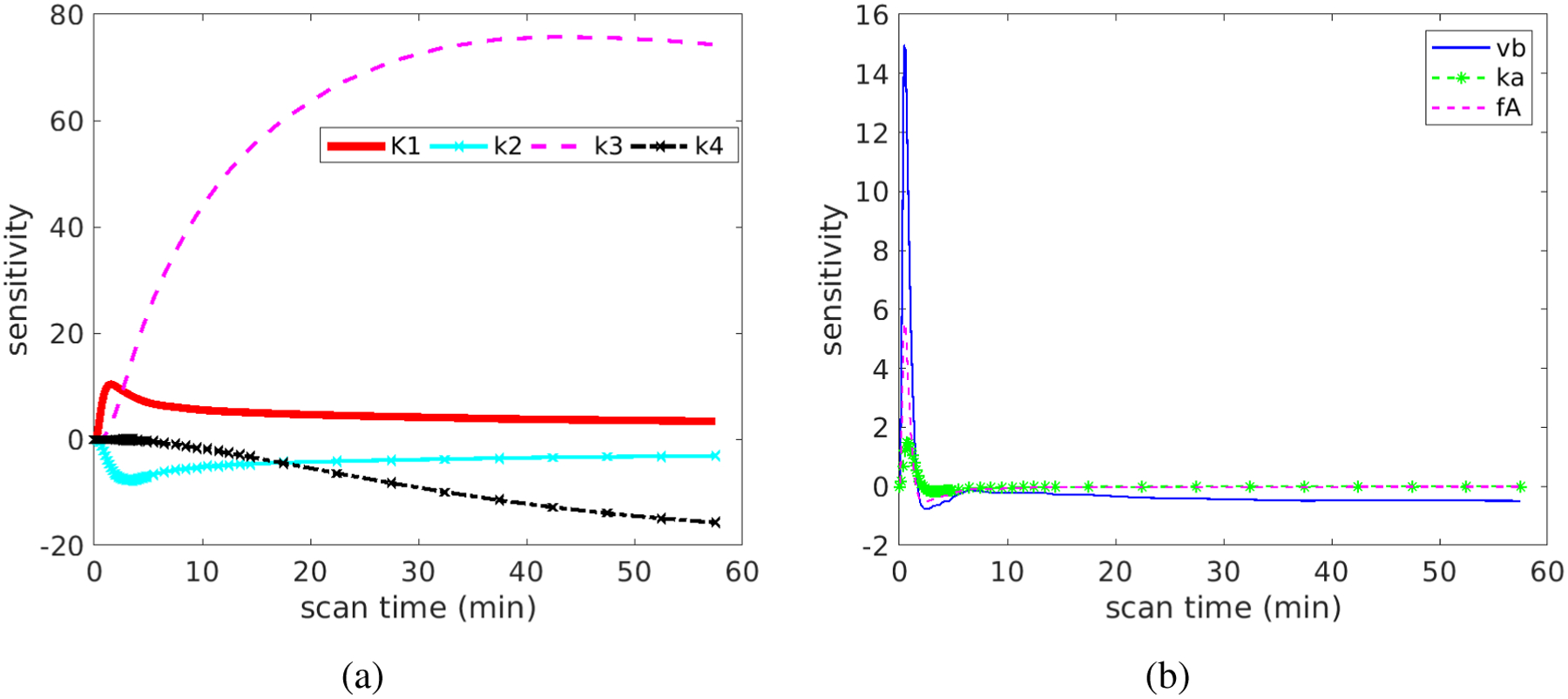
Original sensitivity functions for different kinetic parameters: (a) K1, k2, k3, k4 and (b) vb, ka, fA.
Figure 6 shows the normalized sensitivity functions, which allow a better comparison across different kinetic parameters. In the first 60 minutes, the TAC is more sensitive to K1 and k2 than to k3 and k4. The correlation between the normalized sensitivity functions is summarized in Table 1. The curves of K1 and k2 have opposite signs. Their shapes are similar at late times but are different at early times, resulting in a modest correlation with each other (r = −0.67). A similar effect also holds true between k3 and k4 (r = −0.87). The curve of vb is almost fully overlapped with that of fA, indicating the correlation is high and it is difficult to differentiate them from each other. Because the curve shape of vb or fA is different from the shape of K1, the coupled effect of vb and fA should have a minimal effect on the estimation of K1, as indicated by the small correlation.
Figure 6.
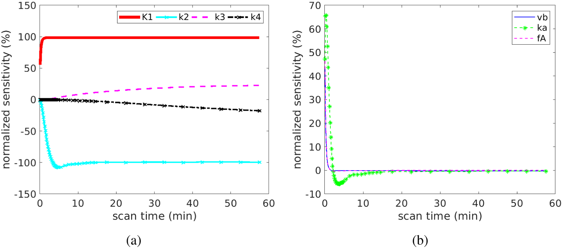
Normalized sensitivity functions for different kinetic parameters: (a) K1, k2, k3, k4 and (b) vb, ka, fA
Table 1.
Correlation matrix of the sensitivity functions.
| K1 | k3 | k4 | k2 | vb | ka | fA | |
|---|---|---|---|---|---|---|---|
| K1 | 1.00 | −0.56 | 0.54 | −0.67 | −0.18 | 0.16 | −0.27 |
| k3 | 1.00 | −0.87 | 0.14 | −0.39 | −0.40 | −0.31 | |
| k4 | 1.00 | −0.33 | 0.21 | 0.18 | 0.13 | ||
| k2 | 1.00 | 0.68 | 0.59 | 0.73 | |||
| vb | 1.00 | 0.79 | 1.00 | ||||
| ka | 1.00 | 0.77 | |||||
| fA | 1.00 |
3.3.2. Determination of the noise model parameter
Figure 7 shows the histograms of the normalized residual error Δcm at the whole-liver ROI level and the liver-segment ROI level. Note that all 49 frames with various scan durations (10s, 60s, 300s) of each patient scan are included for this analysis. The obtained Sc values are 0.3 and 0.6, respectively. The distribution of Δcm approximately follows a Gaussian in both cases. We therefore used these two Sc values to define the noise standard deviation for the whole-liver ROI level and liver-segment level in the simulation studies. Note that the size of whole-liver ROI is 8 times that of the liver-segment ROI, which ideally should reduce the noise standard deviation by a factor of . However, pixels in the liver ROI are not fully independent of each other and therefore the reduction in Sc may be smaller than that suggested by the ROI size increase.
Figure 7.
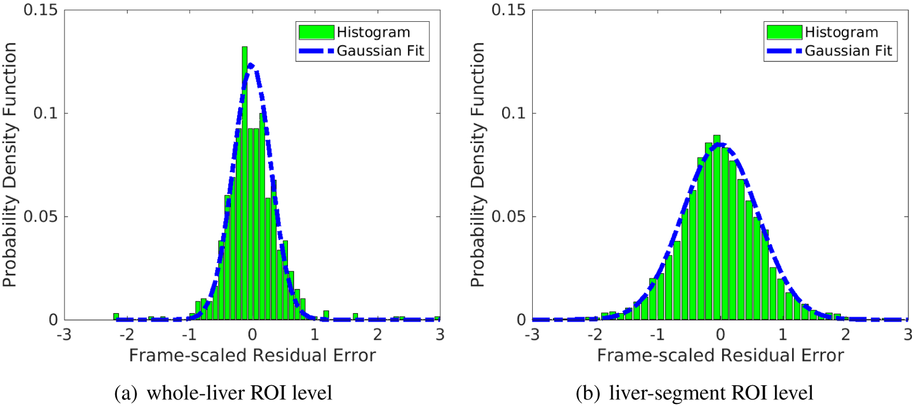
Fit of the histogram of normalized residual difference Δcm using a Gaussian distribution with the standard deviation Sc. (a) whole-liver ROI level, Sc = 0.3; (b) liver-segment ROI level, Sc = 0.6. Note that all time frames of different scan duration are included.
3.3.3. Comparison of different fitting options
Figure 8 shows the comparison of different initialization and weighting schemes for each patient at the whole-liver ROI level (Sc = 0.3). The K1 single-initialization strategy resulted in bias in K1 in several patient datasets. The bias can be reduced when the multi-initialization strategy was used, which however did not provide a universal improvement over all patients. On the other hand, use of nonuniform weighting for TAC fitting led to reduced bias in some patients. The benefit of these two modifications were maximized when they were used together and the bias in K1 remained small in all patients. Thus, the multi-initialization for K1 and nonuniform weighting scheme were used in this work for all subsequent analysis.
Figure 8.
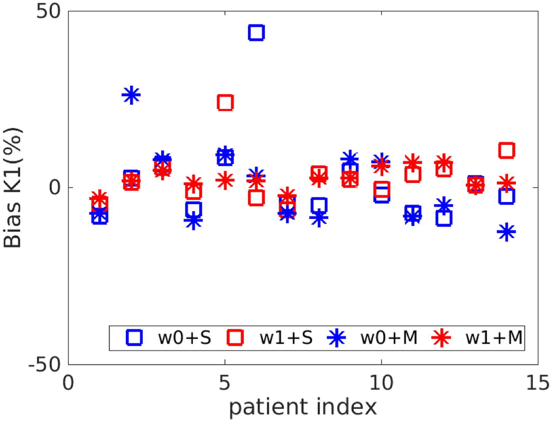
Bias in K1 estimated using different fitting options. S refers to the use of single initial value for K1 and M refers to use multiple initial values. w0 means the uniform weighting scheme and w1 means the nonuniform weighting scheme.
3.3.4. Bias of simplified kinetic models
Figure 9 show the bias and SD of K1 and Ki estimated by three different kinetic models at the noise level of Sc = 0.3. When the traditional SBIF model was used for fitting the TAC, K1 was underestimated with an average 37% bias. K1 by the population-based DBIF was also underestimated by 26%. In comparison, the mean absolute bias of K1 by the optimization-derived DBIF model was only about 3% and the biases of individual patients all remain small. For the estimation of Ki, the SBIF and population-based DBIF resulted in an underestimation of approximately 60%, as compared with an average bias of less than 5% by the optimization-derived DBIF model.
Figure 9.
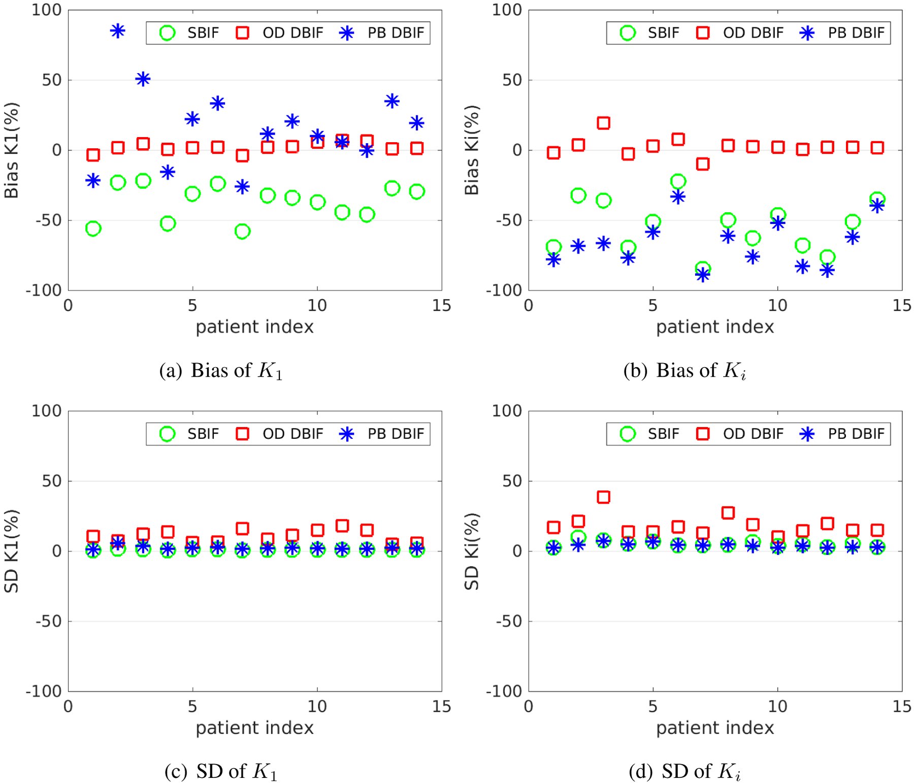
Bias and SD of K1 and Ki estimates in the optimization-derived (OD) DBIF model for 14 patient data sets with Sc = 0.3, as compared with the inaccurate SBIF model and population-based (PB) DBIF model.
The bias reduction achieved by the optimization-derived DBIF model came with the price of increased SD, as shown in Figure 9(c) and (d). The average SD was 11% for K1 and 18% for Ki by the optimization-derived DBIF, as compared to less than 6% by the other two models. This can be explained by the increased number of free parameters in the optimization-derived DBIF model.
The results of the averaged absolute bias and SD across different patients are summarized in table 2 for all FDG transport rate parameters. Generally, with the assumption of the TACs following the DBIF model, the simplified SBIF model resulted in greater than 35–85% bias and the population-based DBIF model led to greater than 20–90% bias in all kinetic estimates. The more accurate optimization-derived DBIF model still had a bias of about 3–8% in all the kinetic estimates, which can be explained by the highly nonlinear noise propagation and by the structural identifiability of the model being local as opposed to global.
Table 2.
Absolute bias and SD of liver FDG kinetic parameter estimates by different kinetic models. The absolute bias and SD are averaged over 14 patient data sets.
| OD DBIF | SBIF | PB DBIF | ||||
|---|---|---|---|---|---|---|
| Bias (%) | SD(%) | Bias(%) | SD(%) | Bias(%) | SD(%) | |
| K1 | 3.2 | 10.8 | 36.7 | 1.1 | 25.5 | 2.6 |
| k2 | 3.5 | 11.6 | 40.1 | 1.1 | 21.7 | 2.4 |
| k3 | 5.0 | 19.7 | 56.1 | 5.2 | 69.4 | 4.0 |
| k4 | 8.1 | 44.0 | 85.1 | 9.4 | 90.7 | 8.5 |
| Ki | 4.5 | 18.3 | 53.8 | 5.2 | 66.1 | 4.2 |
Note that as compared to the simplified SBIF and population-based DBIF models, the increase of SD by the optimization-derived DBIF model was generally smaller than the corresponding bias reduction. This indicates the overall gain of the new model is greater than its loss, as reflected by the RMSE evaluation in table 3. This has led to the improvement in correlating FDG K1 with histology as we observed in the previous patient study [Wang et al., 2018].
Table 3.
RMSE (%) of liver FDG kinetic parameter estimates by different kinetic models. The RMSE is averaged over 14 patient data sets.
| OD DBIF | SBIF | PB DBIF | |
|---|---|---|---|
| RMSE (%) | RMSE (%) | RMSE (%) | |
| K1 | 11.3 | 36.7 | 25.8 |
| k2 | 12.1 | 40.1 | 21.9 |
| k3 | 20.6 | 56.5 | 69.6 |
| k4 | 45.2 | 86.1 | 91.8 |
| Ki | 19.1 | 54.1 | 66.3 |
3.3.5. Effect of neglecting k4
Figure 10 compares the bias and RMSE of K1 and Ki between the two fitting options with free k4 or fixed k4 = 0 for the optimization-derived DBIF model. The averaged bias of K1 over 14 patient data sets was 3.2% versus 11.9% and the averaged bias of Ki was 4.5% and 48.8% for the two options. While with lower SD, the approach with k4 = 0 generally resulted in higher RMSE especially in Ki estimates than the approach with free k4.
Figure 10.
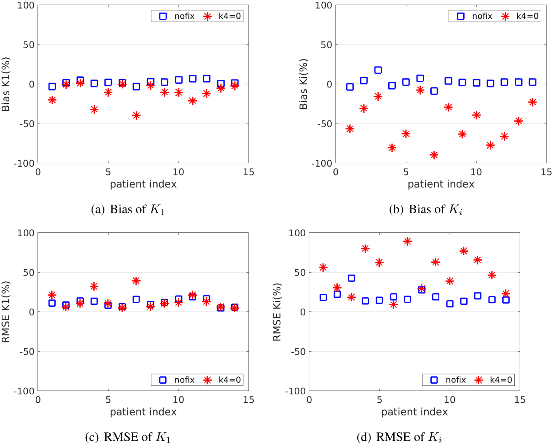
Bias and RMSE of K1 and Ki of the fitting approaches with and without fixing k4 at zero.
3.3.6. Effect of noise levels on kinetic quantification
Table 4 shows the average absolute bias and SD of kinetic parameters estimated by the optimization-derived DBIF model under three noise levels: noise-free (Sc = 0.0), noise at the whole-liver ROI level (Sc = 0.3), and noise at the liver-segment ROI level (Sc = 0.6). While other kinetic parameters had a small bias, the bias of vb and fA were surprisingly large even at the noise-free case (Sc = 0.0). This can be explained by the fact that the model is locally identifiable with potential multiple solutions. The result is also consistent with the observation on the indifferentiable sensitivity curves of vb and fA in figure 5. Despite the large bias in vb and fA, the bias of K1 remained small (<8%). The SD of K1 increased from 7% to 18% when the noise level was changed from the whole-liver ROI level to liver-segment ROI level. The estimation of Ki is more sensitive to noise, with the SD being 18% for the whole-liver ROI level and 37% for the liver-segment ROI level. k2 had similar accuracy and precision as K1 and k3 had similar accuracy and precision as Ki. k4 had a much higher bias and SD because the scan time (1-hour in our study) is not sufficient enough for robust estimation of k4, which can be justified from its sensitivity curve.
Table 4.
Bias and SD of the kinetic parameters in the optimization-derived DBIF model under three different noise levels: Sc = 0 (noise-free), Sc = 0.3 (whole-liver ROI level), and Sc = 0.6 (liver-segment ROI level).
| Sc = 0 | Sc = 0.3 | Sc = 0.6 | ||||
|---|---|---|---|---|---|---|
| Bias (%) | SD(%) | Bias(%) | SD(%) | Bias(%) | SD(%) | |
| K1 | 0.6 | 0 | 3.2 | 10.8 | 7.4 | 18.3 |
| k2 | 0.6 | 0 | 3.5 | 11.6 | 8.2 | 19.6 |
| k3 | 0.2 | 0 | 5.0 | 19.7 | 12.4 | 40.3 |
| k4 | 0.1 | 0 | 8.1 | 44.0 | 22.7 | 81.6 |
| Ki | 0.2 | 0 | 4.5 | 18.3 | 11.1 | 37.0 |
| vb | 16.2 | 0 | 71.8 | 206.5 | 182.6 | 484.6 |
| ka | 0.6 | 0 | 3.9 | 16.2 | 6.1 | 27.6 |
| fA | 16.9 | 0 | 38.3 | 121.9 | 41.6 | 142.5 |
3.3.7. Parameter estimation accuracy over clinical range
Figure 11 shows the plots of linear correlation between the true values and noisy estimates of different kinetic parameters at the whole-liver ROI noise level. The correlation coefficients under different noise levels for all kinetic parameters are summarized in table 5. As the noise level increased, the correlation coefficients reduced. Both K1 and Ki were well repeatable against noise. While all other kinetic parameters including (k2, k3, k4, ka) can be repeated well, the two vascular parameters vb and fA are less repeatable.
Figure 11.
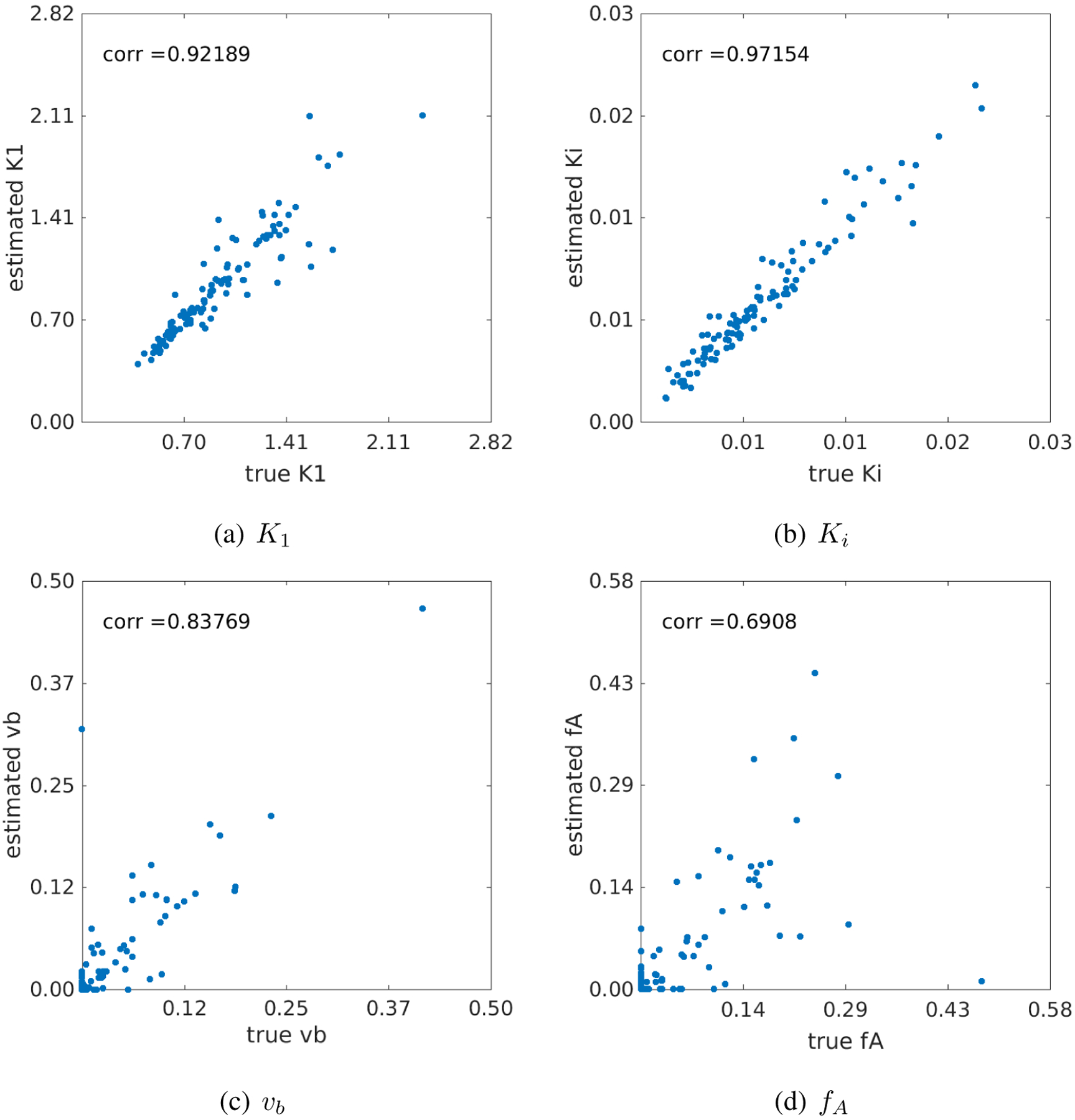
Correlation between the true kinetic parameter values and estimated values from noisy data (Sc = 0.3). (a) K1, (b) Ki, (c) vb and fA.
Table 5.
Coefficients of the linear correlation between estimated kinetic parameters and their true values.
| vb | K1 | k2 | k3 | k4 | ka | fA | Ki | |
|---|---|---|---|---|---|---|---|---|
| Sc = 0.3 | 0.84 | 0.92 | 0.90 | 0.97 | 0.98 | 0.91 | 0.69 | 0.97 |
| Sc = 0.6 | 0.78 | 0.88 | 0.83 | 0.90 | 0.91 | 0.79 | 0.66 | 0.90 |
3.3.8. Noise variation of the K1 correlation with liver inflammation
Figure 12 shows the results of correlating the histological inflammation scores with the FDG K1 estimates derived from 1000 noisy realizations (Sc = 0.3). This investigation quantitates the uncertainty (due to PET measurement noise) associated with the correlation estimation. The Pearson’s correlation r between the original K1 values and liver inflammation scores in the cohort of 14 patients was r =−0.7618 (p=0.0012). The 95% confidence interval of the noisy r estimates was estimated to be [−0.8434, −0.6494] with the mean −0.7452 and standard derivation 0.0493. The percent bias in r was −2.2% and the SD was 6.5%, both approximately close to that in K1. The results indicate the noise stability of the estimation of the correlation between FDG K1 and liver inflammation.
Figure 12.
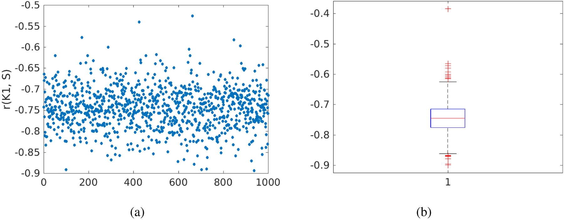
Noise variation of the correlation r between FDG K1 and histological liver inflammation score. (a) r values of 1000 noisy realizations, (b) box plot of the r values.
4. Discussion
FDG K1 by the optimization-derived DBIF model can be a promising PET biomarker for evaluating human liver inflammation in fatty liver disease [Wang et al., 2018, Sarkar et al., 2019, Wang et al., 2017, Sarkar et al., 2017]. A more detailed explanation of the possible physiological hypothesis is provided in our previous work [Sarkar et al., 2019]. The focus of the current work is to characterize the identifiability of the optimization-derived DBIF model structure and evaluate the accuracy and precision of K1 and other kinetic parameters in dynamic liver FDG-PET.
We first conducted a theoretical analysis of the structural identifiability of standard 3-compartmental model and the new DBIF model using the Laplacian transform. While standard 3-compartmental model is globally identifiable, the new model is locally identifiable due to potential multiple solutions. This suggests that particular care should be given to set the initial values as well as the upper and lower bounds such that the kinetic parameter estimation can properly constrain the optimization problem of TAC fitting with the new model.
We then conducted computer simulations to examine the practical identifiability of the model parameters based on 14 patient datasets which include both dynamic FDG-PET data and histopathology data of human liver inflammation. While the estimation of some kinetic parameters (e.g. fA and vb) is associated with large bias and standard deviation, FDG K1, the parameter of major interest, has low bias (≈3%) and standard deviation (≈11%) at the whole-liver ROI level. As demonstrated in the simulation study, fitting liver TACs using the simplified SBIF model or population-based DBIF model may result in significant bias (>20%) in liver K1 quantification. These results explain why the K1 by the new model achieved a statistically significant association with liver inflammation in the patient study, while the other two models did not demonstrate success [Wang et al., 2018].
We also examined the reliability of the new model for liver K1 quantification over a wide range of values from 0.5 to 2.5 (Fig. 11). The true K1 values and their estimates are highly correlated (r > 0.9). The stability of K1 estimation against noise is also preserved in its correlation with liver inflammation (Fig. 12).
We further studied the effect of nonzero k4. Recent interests in whole-body parametric imaging have been growing with the implementation of multi-bed dynamic PET imaging for commercial scanners [Karakatsanis et al., 2013a, Hu et al., 2017] and the advent of total-body PET scanners [Cherry et al., 2017, Badawi et al., 2019]. For parametric imaging of FDG Ki, k4 is usually neglected by standard whole-body Patlak parametric imaging [Karakatsanis et al., 2013a, Karakatsanis et al., 2013b]. Our computer simulation study suggests that k4 should not be neglected in the liver if one-hour scan is used, which is consistent with past dynamic FDG studies [Messa et al., 1992, Okazumi et al., 1992, Miyazawa et al., 1993, Karakatsanis et al., 2014]. Full 3-compartmental modeling or the generalized Patlak method [Karakatsanis et al., 2015] can be thereby used to take into account the effect of nonzero k4 when the liver is involved in the field of view.
A disadvantage of the optimization-derived DBIF model is the increased standard deviation in kinetic parameter estimation, which is basically caused by the increased number of free parameters. To control the standard deviation of K1 and other parameters of interest, one potential strategy is to add additional constraints in the optimization problem. For example, Table 6 compares the bias and standard deviation of kinetic parameters for either estimating or fixing the input function parameter ka in the optimization of TAC fitting. If ka is fixed at its true values, the bias and standard deviation of K1 (and other kinetic parameters) can be largely reduced. This is not surprising because a fixed ka corresponds to a known portal vein input function. However, the result reported here indicates the potential improvement space if a modified method can be developed to incorporate the prior information of the portal vein input function.
Table 6.
Normalized absolute Bias, SD and RMSE of a typical kinetic parameter set (population means) estimated by the optimization-derived DBIF model with ka freely estimated or fixed at its true value.
| free ka | fixed ka | |||||
|---|---|---|---|---|---|---|
| Bias (%) | SD(%) | RMSE(%) | Bias(%) | SD(%) | RMSE(%) | |
| K1 | 3.2 | 10.8 | 11.3 | 0.3 | 3.0 | 3.0 |
| k2 | 3.5 | 11.6 | 12.1 | 0.4 | 3.4 | 3.4 |
| k3 | 5.0 | 19.7 | 20.6 | 1.9 | 17.7 | 17.9 |
| k4 | 8.1 | 44.0 | 45.2 | 4.6 | 41.6 | 42.1 |
| Ki | 4.5 | 18.3 | 19.1 | 1.7 | 16.6 | 16.7 |
| vb | 71.8 | 206.5 | 158.1 | 47.9 | 116.9 | 91.0 |
| ka | 3.9 | 16.2 | 16.8 | / | / | / |
| fA | 38.3 | 121.9 | 93.6 | 40.0 | 106.0 | 81.4 |
The study also indicates that kinetic quantification at the liver-segment ROI noise level (Sc = 0.6) is less reliable than at the whole-liver ROI noise level (Sc = 0.3). Both bias and SD become nearly doubled, as shown in Table 4. It is worth noting that all the studies were conducted using standard clinical PET. The high-sensitivity EXPLORER scanner can increase sensitivity of PET by a factor of 4–5 for imaging a single organ [Poon et al., 2012, Cherry et al., 2018, Zhang et al., 2017, Badawi et al., 2019], which can reduce the liver-segment ROI noise level from current Sc = 0.6 to Sc = 0.3, i.e., by a factor equal to the square-root of the sensitivity improvement, which is estimated to be approximately a factor of 4 for single-organ imaging. Thus, quantification of liver segmental heterogeneity may become reliable on EXPLORER. Equivalently, the whole-liver ROI noise level may also be reduced from current Sc = 0.3 to Sc = 0.15 if EXPLORER is used. The resulting bias and SD of K1 were 1.4% and 6.5%, respectively, according to our simulation study using Sc = 0.15.
This study has limitations. While the Monte Carlo-based 1D computer simulation approach used in this work is not different from other studies of kinetic modeling (e.g., [Wu and Carson, 2002]), the approach simulated the noise of TACs in the temporal domain but neglected potential spatial correlations of the noise. A fully 4D Monte Carlo simulation (e.g., by GATE) can be more realistic, though we do not expect that it would result in a significant difference in TAC noise modeling. The nonlinear least-square fitting in this work was solved by the classic Levenberg-Marquardt optimization algorithm, which only finds local solutions. Our preliminary study of multi-initialization indicated that a better optimization search could be beneficial. Thus, our future work will include the development of an improved optimization algorithm for this application. In addition, the model needs to be further modified if kinetic parameters (e.g., vb) other than K1 and Ki are of interest. A possible solution could be to include the gut compartment in a way similar to [Garbarino et al., 2015].
5. Conclusion
This paper has conducted both theoretical analysis of structural identifiability and computer study of practical identifiability for the optimization-derived DBIF model in dynamic PET of liver inflammation. The theoretical analysis suggests that the parameters of the new model are identifiable but subject to local solutions. The simulation results have shown that the estimation of vascular kinetic parameters (vb and fA) suffer from high variation. However, FDG K1 can be reliably estimated in the new optimization-derived DBIF model. The bias of K1 by the new model is approximately 3% and the standard deviation is about 11% at the whole-liver ROI noise level. The estimated values of K1 are also highly correlated with the original K1 values (r = 0.92). The correlation between liver FDG K1 by the new model and histological inflammation score is robust to noise interference. These results suggest that liver FDG K1 quantification is reliable for clinical use to assess liver inflammation at the whole-liver ROI level. Future work will include further development of the DBIF modeling and optimization approaches and use of EXPLORER for reduced bias and variance in K1.
Acknowledgment
The authors thank the anonymous reviewers for their helpful comments. The work of G. Wang was supported in part by the UC Davis Comprehensive Cancer Center under NIH Grant P30 CA093373 and K12 Dean’s Scholar Award.
6. Appendix
6.1. Structural identifiability of single-input kinetic model
Substituting equations (4) – (9) into equation (20), we have
| (37) |
| (38) |
where the coefficients are defined by
| (39) |
| (40) |
| (41) |
| (42) |
| (43) |
Using the equation set αi = Di and βi = Ni, we can obtain a unique solution for θ after some algebraic operations:
| (44) |
| (45) |
| (46) |
| (47) |
| (48) |
Therefore, the traditional SBIF three-compartmental model structure is globally identifiable in the parameter space.
6.2. Derivation of the structural identifiability of dual-input kinetic modeling
Similarly, for the optimization-derived DBIF model, the numerator and denominator of the transfer function Φ(s) are given by
| (49) |
| (50) |
where {αi, βi} are defined by equations (39)–(43). The equation set to determine θ is:
| (51) |
| (52) |
| (53) |
| (54) |
| (55) |
| (56) |
| (57) |
Using equations (51) – (53), we obtain Eq. (26) for ka. Using equations (54) – (57), we obtain Eq. (27) for fA.
References
- Anderson D (1983). Compartmental Modeling and Tracer Kinetics Lecture Notes in Biomathematics. Springer Berlin Heidelberg. [Google Scholar]
- Badawi RD, Shi H, Hu P, Chen S, Xu T, Price PM, Ding Y, Spencer BA, Nardo L, Liu W, Bao J, Jones T, Li H, Cherry SR (2019). First Human Imaging Studies with the EXPLORER Total-Body PET Scanner. Journal of Nuclear Medicine, 60(3): 299–303. [DOI] [PMC free article] [PubMed] [Google Scholar]
- Bellman R and Astrom KJ (1970). On structural identifiability. Mathematical Biosciences, 7:329–339. [Google Scholar]
- Brix G, Ziegler SI, Bellemann ME, Doll J, Schosser R, Lucht R, Krieter H, Nosske D, and Haberkorn U (2001). Quantification of [F-18]FDG uptake in the normal liver using dynamic PET: Impact and modeling of the dual hepatic blood supply. Journal of Nuclear Medicine, 42(8):1265–1273. [PubMed] [Google Scholar]
- Carson RE, Yan Y, Daubewitherspoon ME, Freedman N, Bacharach SL, and Herscovitch P (1993). An approximation formula for the variance of PET region-of-interest values. IEEE Transactions on Medical Imaging, 12(2):240–250. [DOI] [PubMed] [Google Scholar]
- Cherry SR, Badawi RD, Karp JS, Moses WW, Price P, and Jones T (2017). Total-body imaging: Transforming the role of positron emission tomography. Science Translational Medicine, 9(381). [DOI] [PMC free article] [PubMed] [Google Scholar]
- Cherry SR, Jones T, Karp JS, Qi JY, Moses WW, and Badawi RD (2018). Total-body PET: Maximizing sensitivity to create new opportunities for clinical research and patient care. Journal of Nuclear Medicine, 59(1):3–12. [DOI] [PMC free article] [PubMed] [Google Scholar]
- Delbary F, Garbarino S, Vivaldi V, (2010). Compartmental analysis of dynamic nuclear medicine data: models and identifiability. Inverse Problems, 32(12):125010 (24pp). [Google Scholar]
- Doot RK, Muzi M, Peterson LM, Schubert EK, Gralow JR, Specht JM, and Mankoff DA (2010). Kinetic analysis of 18f-fluoride PET images of breast cancer bone metastases. J Nucl Med, 51(4):521–7. [DOI] [PMC free article] [PubMed] [Google Scholar]
- El Fakhri G, Kardan A, Sitek A, Dorbala S, Abi-Hatem N, Lahoud Y, Fischman A, Coughlan M, Yasuda T, and Di Carli MF (2009). Reproducibility and accuracy of quantitative myocardial blood flow assessment with 82Rb PET: comparison with 13N-ammonia PET. Journal of Nuclear Medicine, 50(7):1062–1071. [DOI] [PMC free article] [PubMed] [Google Scholar]
- Garbarino S, Vivaldi V, Delbary F, Caviglia G, Piana M, Marini C, Capitanio S, Calamia I, Buschiazzo A, and Sambuceti G (2015). A new compartmental method for the analysis of liver FDG kinetics in small animal models. EJNMMI Research, 5(1): 107. [DOI] [PMC free article] [PubMed] [Google Scholar]
- Gunn R (1996). Mathematical modelling and identifiability applied to positron emission tomography data. PhD thesis, University of Warwick. [Google Scholar]
- Hu J, Panin V, Smith AM, WH, Shah Vijay, Kehren F, and Casey M (2017), Clinical whole body CBM parametric PET with flexible scan modes, Conference Record of IEEE Nuclear Science Symposium and Medical Imaging Conference, 2017. [Google Scholar]
- Kalman RE (1963). Mathematical description of linear dynamical systems. Journal of the Society for Industrial and Applied Mathematics Series A Control, 1(2):152–192. [Google Scholar]
- Karakatsanis NA, Lodge MA, Casey ME, Zaidi H, and Rahmim A (2014). Impact of acquisition time-window on clinical whole-body PET parametric imaging. 2014 IEEE Nuclear Science Symposium and Medical Imaging Conference. [Google Scholar]
- Karakatsanis NA, Lodge MA, Tahari AK, Zhou Y, Wahl RL, and Rahmim A (2013a). Dynamic whole-body PET parametric imaging: I. concept, acquisition protocol optimization and clinical application. Physics in Medicine and Biology, 58(20):7391–7418. [DOI] [PMC free article] [PubMed] [Google Scholar]
- Karakatsanis NA, Lodge MA, Zhou Y, Wahl RL, and Rahmim A (2013b). Dynamic whole-body PET parametric imaging: II. task-oriented statistical estimation. Physics in Medicine and Biology, 58(20):7419–7445. [DOI] [PMC free article] [PubMed] [Google Scholar]
- Karakatsanis NA, Zhou Y, Lodge MA, Casey ME, Wahl RL, Zaidi H, and Rahmim A (2015). Generalized whole-body patlak parametric imaging for enhanced quantification in clinical PET. Physics in Medicine and Biology, 60(22):8643–8673. [DOI] [PMC free article] [PubMed] [Google Scholar]
- Keiding S (2012). Bringing Physiology into PET of the Liver. Journal of Nuclear Medicine, 53:425–433. [DOI] [PMC free article] [PubMed] [Google Scholar]
- Keramida G, Potts J, Bush J, Dizdarevic S, Peters AM. (2014a). Hepatic steatosis is associated with increased hepatic FDG uptake. European Journal of Radiology, 83:751–755. [DOI] [PubMed] [Google Scholar]
- Keramida G, Potts J, Bush J, Verma S, Dizdarevic S, Peters AM. (2014b). Accumulation of F-18-FDG in the Liver in Hepatic Steatosis. American Journal of Roentgenology, 203:643–648. [DOI] [PubMed] [Google Scholar]
- Komorowski M, Costa MJ, Rand DA, and Stumpf MP (2011). Sensitivity, robustness, and identifiability in stochastic chemical kinetics models. Proc Natl Acad Sci U S A, 108(21):8645–50.21551095 [Google Scholar]
- Kudomi N, Jarvisalo MJ, Kiss J, Borra R, Viljanen A, Viljanen T, Savunen T, Knuuti J, Iida H, Nuutila P, and Iozzo P (2009). Non-invasive estimation of hepatic glucose uptake from [18F]FDG PET images using tissue-derived input functions. Eur J Nucl Med Mol Imaging, 36(12):2014–26. [DOI] [PubMed] [Google Scholar]
- Lee SS, Park SH (2014). Radiologic evaluation of nonalcoholic fatty liver disease. World Journal of Gastroenterology, 20:7392–7402. [DOI] [PMC free article] [PubMed] [Google Scholar]
- Mankoff D, Muzi M, and Zaidiy H (2006). Quantitative analysis in nuclear oncologic imaging In Quantitative Analysis in Nuclear Medicine Imaging, pages 494–536. Springer. [Google Scholar]
- Mankoff DA, Shields AF, Graham MM, Link JM, Eary JF, and Krohn KA (1998). Kinetic analysis of 2-[carbon-11]thymidine PET imaging studies: compartmental model and mathematical analysis. J Nucl Med, 39(6):1043–55. [PubMed] [Google Scholar]
- Messa C, Choi Y, Hoh CK, Jacobs EL, Glaspy JA, Rege S, Nitzsche E, Huang SC, Phelps ME, and Hawkins RA (1992). Quantification of glucose utilization in liver metastases: parametric imaging of FDG uptake with PET. J Comput Assist Tomogr, 16(5):684–9. [DOI] [PubMed] [Google Scholar]
- Miao H, Dykes C, Demeter LM, Cavenaugh J, Park SY, Perelson AS, and Wu H (2008). Modeling and estimation of kinetic parameters and replicative fitness of HIV-1 from flow-cytometry-based growth competition experiments. Bulletin of Mathematical Biology, 70(6):1749–1771. [DOI] [PMC free article] [PubMed] [Google Scholar]
- Miao H, Xia X, Perelson AS, and Wu H (2011). On identifiability of nonlinear ODE models and applications in viral dynamics. SIAM Rev Soc Ind Appl Math, 53(1):3–39. [DOI] [PMC free article] [PubMed] [Google Scholar]
- Michelotti GA, Machado MV, and Diehl AM (2013). NAFLD, NASH and liver cancer. Nat Rev Gastroenterol Hepatol, 10(11):656–65. [DOI] [PubMed] [Google Scholar]
- Miyazawa H, Osmont A, Petit-Taboue MC, Tillet I, Travere JM, Young AR, Barre L, MacKenzie ET, and Baron JC (1993). Determination of 18f-fluoro-2-deoxy-d-glucose rate constants in the anesthetized baboon brain with dynamic positron tomography. J Neurosci Methods, 50(3):263–72. [DOI] [PubMed] [Google Scholar]
- Mourik JE, Lubberink M, Klumpers UM, Comans EF, Lammertsma AA, Boellaard R. (2008). Partial volume corrected image derived input functions for dynamic PET brain studies: methodology and validation for [11C]flumazenil. Neuroimage, 39(3):1041–50. [DOI] [PubMed] [Google Scholar]
- Munk OL, Bass L, Roelsgaard K, Bender D, Hansen SB, and Keiding S (2001). Liver kinetics of glucose analogs measured in pigs by PET: Importance of dual-input blood sampling. Journal of Nuclear Medicine, 42(5):795–801. [PubMed] [Google Scholar]
- Musso G, Gambino R, Cassader M, and Pagano G (2011). Meta-analysis: natural history of non-alcoholic fatty liver disease (NAFLD) and diagnostic accuracy of non-invasive tests for liver disease severity. Ann Med, 43(8):617–49. [DOI] [PubMed] [Google Scholar]
- Muzi M, Mankoff DA, Grierson JR, Wells JM, Vesselle H, and Krohn KA (2005). Kinetic modeling of 3’-deoxy-3’-fluorothymidine in somatic tumors: mathematical studies. J Nucl Med, 46(2):371–80. [PubMed] [Google Scholar]
- Muzi M, Spence AM, O’Sullivan F, Mankoff DA, Wells JM, Grierson JR, Link JM, and Krohn KA (2006). Kinetic analysis of 3’-deoxy-3’−18f-fluorothymidine in patients with gliomas. J Nucl Med, 47(10):1612–21. [PubMed] [Google Scholar]
- Okazumi S, Isono K, Enomoto K, Kikuchi T, Ozaki M, Yamamoto H, Hayashi H, Asano T, and Ryu M (1992). Evaluation of liver tumors using fluorine-18-fluorodeoxyglucose PET: characterization of tumor and assessment of effect of treatment. J Nucl Med, 33(3):333–9. [PubMed] [Google Scholar]
- Oppenheim AV, Willsky AS, and Nawab SH (1996). Signals &Amp; Systems (2Nd Ed.). Prentice-Hall, Inc., Upper Saddle River, NJ, USA. [Google Scholar]
- Poon JK, Dahlbom ML, Moses WW, et al. (2012). Optimal whole-body PET scanner configurations for different volumes of LSO scintillator: a simulation study solution. Phys Med Biol, 57:4077–4094. [DOI] [PMC free article] [PubMed] [Google Scholar]
- Sarkar S, Corwin M, Olson K, Stewart S, Johnson CR, Badawi R, and Wang GB (2017). 4D dynamic FDG-PET correlates with hepatic inflammation and steatosis in patients with non-alcoholic steatohepatitis. Hepatology, 66:107a–108a. (abstract) [Google Scholar]
- Sarkar S, Corwin M, Olson K, Stewart S, Liu C, Badawi R, and Wang G (2019). Pilot study to diagnose non-alcoholic steatohepatitis with dynamic 18F-fluorodeoxyglucose positron emission tomography. American Journal of Roentgenology, 212(3): 529–537, 2019. [DOI] [PubMed] [Google Scholar]
- Tsien H (1954). Engineering Cybernetics. McGraw-Hill book Company, Incorporated. [Google Scholar]
- Wang G, Corwin M, Olson K, Stewart S, Zha C, Badawi R, and Sarkar S (2017). Dynamic FDG-PET study of liver inflammation in non-alcoholic fatty liver disease. Journal of Hepatology, 66(1):S592 (abstract) [Google Scholar]
- Wang G, Corwin MT, Olson KA, Badawi RD, and Sarkar S (2018). Dynamic PET of human liver inflammation: impact of kinetic modeling with optimization-derived dual-blood input function. Physics in Medicine and Biology, 63(15):155004. [DOI] [PMC free article] [PubMed] [Google Scholar]
- Winterdahl M, Munk OL, Sorensen M, Mortensen FV, Keiding S. (2011). Hepatic Blood Perfusion Measured by 3-Minute Dynamic F-18-FDG PET in Pigs. Journal of Nuclear Medicine, 52:1119–1124. [DOI] [PMC free article] [PubMed] [Google Scholar]
- Wree A, Broderick L, Canbay A, Hoffman HM, and Feldstein AE (2013). From NAFLD to NASH to cirrhosis-new insights into disease mechanisms. Nat Rev Gastroenterol Hepatol, 10(11):627–36. [DOI] [PubMed] [Google Scholar]
- Wu YJ and Carson RE (2002). Noise reduction in the simplified reference tissue model for neuroreceptor functional imaging. Journal of Cerebral Blood Flow and Metabolism, 22(12):1440–1452. [DOI] [PubMed] [Google Scholar]
- Xie L, Yui J, Hatori A, Yamasaki T, Kumata K, Wakizaka H, Yoshida Y, Fujinaga M, Kawamura K, Zhang MR. (2012). Translocator protein (18 kDa), a potential molecular imaging biomarker for non-invasively distinguishing non-alcoholic fatty liver disease. J Hepatol. , 57(5):1076–82. [DOI] [PubMed] [Google Scholar]
- Zhang XZ, Zhou J, Cherry SR, Badawi RD, and Qi JY (2017). Quantitative image reconstruction for total-body PET imaging using the 2-meter long explorer scanner. Physics in Medicine and Biology, 62(6):2465–2485. [DOI] [PMC free article] [PubMed] [Google Scholar]