Effects of long-term exposure to air pollutants on the spatial spread of COVID-19 in Catalonia, Spain

Abstract

Background

The risk of infection and death by COVID-19 could be associated with a heterogeneous distribution at a small area level of environmental, socioeconomic and demographic factors. Our objective was to investigate, at a small area level, whether long-term exposure to air pollutants increased the risk of COVID-19 incidence and death in Catalonia, Spain, controlling for socioeconomic and demographic factors.

Methods

We used a mixed longitudinal ecological design with the study population consisting of small areas in Catalonia for the period February 25 to May 16, 2020. We estimated Generalized Linear Mixed models in which we controlled for a wide range of observed and unobserved confounders as well as spatial and temporal dependence.

Results

We have found that long-term exposure to nitrogen dioxide (NO₂) and, to a lesser extent, to coarse particles (PM₁₀) have been independent predictors of the spatial spread of COVID-19. For every 1 μm/m³ above the mean the risk of a positive test case increased by 2.7% (95% credibility interval, ICr: 0.8%, 4.7%) for NO₂ and 3.0% (95% ICr: -1.4%,7.44%) for PM₁₀. Regions with levels of NO₂ exposure in the third and fourth quartile had 28.8% and 35.7% greater risk of a death, respectively, than regions located in the first two quartiles.

Conclusion

Although it is possible that there are biological mechanisms that explain, at least partially, the association between long-term exposure to air pollutants and COVID-19, we hypothesize that the spatial spread of COVID-19 in Catalonia is attributed to the different ease with which some people, the hosts of the virus, have infected others. That facility depends on the heterogeneous distribution at a small area level of variables such as population density, poor housing and the mobility of its residents, for which exposure to pollutants has been a surrogate.

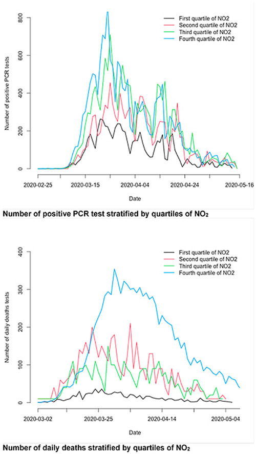
Graphical abstract

Number of positive PCR test stratified by quartiles of NO₂. Number of daily deaths stratified by quartiles of NO_2.

1. - Introduction

The Severe Acute Respiratory Syndrome CoronaVirus 2 (SARS-CoV-2) first appeared in the city of Wuhan, China, in December 2019, and then spread worldwide (Chen et al., 2020; WHO, 2020). By July 8, 2020, 210 countries and territories had been affected, 11,801,805 people diagnosed and 543,902 have died as a result of Coronavirus disease 2019 (COVID-19) (ECDC, 2020).

The main route of transmission for COVID-19 is by the direct or indirect contact with an infected subject through the small droplets that occur when an infected person coughs or sneezes (Domingo et al., 2020). It is also transmitted by touching the eyes, nose, or mouth after touching contaminated surfaces. Therefore, aerosols can play a role in the transmission of COVID-19 (Asadi et al., 2020). People with COVID-19 have reported a wide range of symptoms (fever, cough, shortness of breath, fatigue, headache, loss of taste or smell, sore throat, congestion, nausea, vomiting, and diarrhoea) ranging from mild symptoms to severe illness (CDC, 2019). Several studies have already reported that the age and underlying diseases, mainly cardiovascular, are the most important risk factors for death by COVID-19 (Li X et al., 2020; Onder et al., 2020).

Both incidence and mortality vary greatly between continents, countries and even regions within each country. There have been several factors that could explain the substantial differences in the incidence and mortality rates between affected countries and geographic regions, including, but not limited to, environmental variables and demographic and socioeconomic factors.

At the end of June 2020 we conducted a search in the online databases PubMed, Web of Science, Scopus and Google Scholar, by combining the keyword ‘COVID 19′ with the keywords, ‘environment’, '(environmental factors)', '(air pollution)', ‘socioeconomic’, '(socioeconomic variables)', ‘demographic’ or '(demographic variables)'. After excluding the repetitions, as well as preprints (studies that have not yet been peer-reviewed), qualitative studies, editorials, opinion and purely narrative papers, we were left with 22 studies. Twelve studies evaluated the association of COVID-19 with air pollution and 12 with demographic and socioeconomic variables (two of them also evaluated air pollution). However, of those 22 only 12 (seven of which evaluate air pollution, six socioeconomic and demographic variables and one which evaluates both) used regression models, that is, adjust the associations by some confounders. In fact, and as Bontempi et al. (2020) point out, a pandemic is a complex phenomenon, involving many variables and it cannot be assessed in a bivariate way. The rest of the studies were either purely descriptive (interpretation of bar plots, scatter plots and maps) and/or interpreted correlations, without adjusting for any confounder.

All studies that evaluated the association between the exposure to air pollutants (particulate matter, nitrogen dioxide, ozone and air quality index) and COVID-19 found positive and statistically significant associations, even controlling for possible confounders (especially meteorological variables and only in two of the studies also demographic and socioeconomic factors). In relation to long-term (i.e. chronic) exposure to air pollutants (measured as the spatial variation of air pollutants in a given geographic area over a relatively long period of time), Fattorini and Regoli (2020) (in 71 Italian provinces) and Coccia (2020) (in the 55 Italian cities he studied) found that exposure to air pollutants was significantly associated with an increase in the number of cumulative cases of COVID-19. With regard to short-term (i.e. acute) exposure (measured as the temporal variation of air pollutants), Xu et al. (2020) (in 33 locations in China), Zhu et al. (2020) (in 120 cities in China), Jiang et al. (2020) (3 cities in China), Li H et al. (2020) (2 cities in China) and Adhikari et al. (2020) (in Queens, New York) found significantly positive associations between the short-term exposure to air pollutants with newly confirmed cases. Furthermore, as Domingo et al. (2020) point out, in a very recent review, the results of most of the studies suggest that the long-term exposure to air pollutants might lead to more severe and lethal forms of COVID-19.

Most of the studies evaluating socioeconomic and demographic variables (four of the six studies) considered population density (Coccia, 2020; Ahmadi et al., 2020; Pequeno et al., 2020; and You et al. 2020). Three studies evaluated the influence of income (Azar et al., 2020; You et al., 2020; and Price-Haywood et al., 2020). You et al. (2020) considered the percentage of the population aged 65 or over and the ratio of total floor area to the number of residential buildings. Bontempi (2020a) considered the role of commercial exchanges, as a proxy for social interactions.

In Spain, the region of Catalonia has been the second most affected by the COVID-19 pandemic (the Madrid region being the most affected), both by number of cases (63,042 cases, 25% of all cases in Spain, 821.37 cases per 100,000 inhabitants – 537.17 cases per 100,000 in Spain), and by deaths (5675 deaths, 20% of all deaths in Spain, 73.94 deaths per 100,000 inhabitants – 60.49 deaths per 100,000 in Spain) (Secretaría General de Sanidad, 2020; INE, 2020a). The geographical distribution of the spread of the pandemic has not been spatially homogeneous in the Catalan territory either, and important differences at the small area level have been observed.

Catalonia is mainly an urban region. Sixty percent of the population reside in 23 cities with more than 50,000 inhabitants (comprising 6.62% of the total Catalan territory) and 52% in 14 cities with more than 100,000 inhabitants (comprising 4.64% of the territory) (IDESCAT, 2020). Among these include the second-largest city in Spain, Barcelona, and the 36 adjacent municipalities making up the Barcelona Metropolitan Area, i.e. 41.75% of the population of Catalonia (representing only 1.97% of the territory). All have a high population density and exhibit different levels of urban air pollution whose primary source of emission is from road traffic.

Our hypothesis is that the heterogeneity in the spatial distribution of the pandemic could be attributed to the fact that the risk of infection and death by COVID-19 could be associated with, on the one hand, a heterogeneous distribution at a small area level of environmental factors and, on the other hand, to different socioeconomic and demographic factors in each of those small areas.

Our objective in this paper was to investigate, at a small area level and controlling for socioeconomic and demographic factors, whether long-term exposure to air pollutants, such as particulate matter (PM₁₀, coarse particles with a diameter of 10 μm or less) and nitrogen dioxide (NO₂), increased the risk of COVID-19 incidence and death in Catalonia, Spain.

This work presents as novelties, the use of spatio-temporal models to evaluate the effects of long-term exposure to air pollutants on the spatial spread of COVID-19. In the models we control for a wide range of confounders, both observed and unobserved, and for spatial and temporal dependence. Finally, we have exclusively used open data.

2. - Methods

2.1. - Study area and study period

We used a mixed longitudinal ecological design, in which the response variables were observed several times at different points in time for each small area involved in the study.

The study population consisted of small areas of Catalonia: for incidence, the Basic Health Area (ABS, for its acronym in Catalan from here on) and for mortality the ‘comarca’, an administrative territorial division of Catalonia (region, hereinafter). The study period was between February 25 and May 16, 2020. The design was unbalanced, since neither the ABSs nor the regions were observed the same number of times.

Catalan health planning defines an ABS as the elementary territorial unit through which primary health care services are organized (Atenció Primària Girona, 2020). The ABSs are either made up of neighbourhoods or districts in urban areas or by one or more municipalities in rural areas. Their delimitation is determined by geographical, demographic, social and epidemiological factors and, in particular, based on the accessibility the population has to services and the efficiency in the organization of health resources (Atenció Primària Girona, 2020). Each ABS has a Primary Care Team, consisting of general practitioners, paediatricians, dentists, nurses and nursing assistants, social workers and administrative support staff. Depending on the size of the ABS, the number of municipalities and the dispersion of the population, the ABS will have one Primary Care Centre (CAP) and may have more clinics that are organically dependent on the CAP (Atenció Primària Girona, 2020). Specifically, we considered 372 of the 378 ABSs in Catalonia (because in six of the ABSs no positive test was reported), with a population between 371 and 72,321 inhabitants (mean 20,266 inhabitants, standard deviation 13,391, median 18,457 inhabitants, first quartile -Q1- 10,554, third quartile -Q3- 27,529). The population density was in the range of 0.31–34,590.58 inhabitants/km² (mean 3486.36, standard deviation 6719.23, median 309.18, Q1 44.83, Q3 3752.54). Of the 178 municipalities considered, 46 were divided into more than one ABS, 37 of them into a maximum of five ABSs, eight between six and 14 ABSs and one, (the city of Barcelona) into 67 ABSs (IDESCAT, 2020).

To avoid the identification of the deceased and to guarantee their confidentiality, no cases of mortality are provided at the level of the ABS but rather at the ‘region’ level (Open Government, 2020). We had mortality data for all 42 regions of Catalonia, with a population between 3802 and 2,252,862 inhabitants (mean 176,556 inhabitants, standard deviation 376,639, median 50,943 inhabitants, Q1 19,739, Q3 171,874). The population density was in the range 0.36–3997. inhabitants/km² (mean 170.38, standard deviation 642.44, median 30.63, Q1 11.16, Q3 83.52) (IDESCAT, 2020).

2.2. - Measures of the study, data and sources

2.2.1. Outcome variables

To evaluate the incidence, we used daily incident positive cases, which were those that tested positive on some diagnostic test (PCR or fast test) (Open Government, 2020), at the level of the ABS. For mortality we used daily deaths obtained from the funeral homes’ reports to the Catalan Health Department (Open Government, 2020). These reports declare positive cases as well as suspicious ones. Suspicious cases corresponded to people who presented symptoms at some point and a health professional classified them as a possible case, but they did not have a diagnostic test with a positive result. All data were obtained from the RSAcovid19 records from the Catalan Health Department (Open Government, 2020).

2.2.2. Air pollutants

We used long-term exposure to air pollutants, particulate matter (PM₁₀) and nitrogen dioxide (NO₂) in each of small areas from 2011 to 2019.

It is important to note that we evaluated long-term exposure to these air pollutants. That is to say, a subject, by virtue of residing in a certain small area, has been exposed to an (average) level of various environmental variables in the small area where, in our case, they resided at least during the period 2011–2019. We were interested in the effects that geographical variation of such exposure may have on the spatial spread of COVID-19.

We obtained information on the levels of air pollution for 2011–2019 from the 144 monitoring stations in the Catalan Network for Pollution Control and Prevention (XVPCA) located throughout Catalonia (Dades obertes Catalunya, 2020). We predicted the levels of air pollutants to which the inhabitants of each ABS and each region had been exposed to from 2011 to 2019 using a joint Bayesian model. The dependent variables were PM₁₀ and NO₂. As explanatory variables we included air pollutants other than the dependent variable (fine particles with a diameter of 2.5 μm or less -PM_2.5- nitrogen oxide -NO-, sulphur dioxide -SO₂-, carbon monoxide -CO-, ozone -O₃-, benzene -C₆H₆-, benzopyrene -B-, lead, arsenic, nickel, cadmium; in addition to PM₁₀ and NO₂ when the dependent variable was NO₂ and PM₁₀, respectively) and the surface of the ABS or the region. In the model we controlled for spatial heterogeneity and both spatial and temporal dependence. This model allowed us to avoid the problems caused by spatial misalignment. If this problem is not corrected properly (as we did), there will be a complex form of measurement error leading to biased (i.e. asymptotically biased) and inconsistent estimates and erroneous standard errors in the estimates of the parameters. Further details concerning this can be found in Barceló et al. (2016).

In fact, although PM₁₀ was observed at stations located at only 94 of the 372 ABSs and NO₂ at 66 of them, the model fit was very good in both cases (Figs. A1 and A2 in supplementary material).

2.2.3. Control variables

We controlled for socioeconomic and demographic variables in the last year (or period) available at the census tract level (the only small area below the municipality for which data are provided). In particular:

Average income per person (in Euros). Average of the years 2015, 2016 and 2017. Variable observed at the census track level (Source: Instituto Nacional de Estadística, INE, 2020b).

Unemployment rate in 2011 (in percentages). Variable observed at the census track level (Source: Spanish Population and Housing Census 2011, INE, 2011).

Percentage of population aged 65 and over in 2019. Variable observed at the census track level (Source: INE, 2020a).

Percentage of foreigners in 2019 from countries with medium and low human development index according to the United Nations Development UNDP. United Nations Development Program (2019). Variable observed at the census track level (Source: INE, 2020a).

Poor housing. Percentage of houses with less than 45 m² of living area in 2011. Variable observed at the census track level (Source: Spanish Population and Housing Census 2011, INE, 2011).

Percentage of single person households in 2017. Variable observed at the census track level (Source: INE, 2020n).

Population density in 2019 (in inhabitants/km²). Variable observed at both, ABS and region level (Source: INE, 2020a, and Statistical Institute of Catalonia, IDESCAT, 2020).

With the exception of population density, all other variables were observed at the census tract level. Using the population of each of the census tracts as weights (the source of the total population of the census tract and of the population of the census tract by sex was INE (2020a) we calculated the weighted average of the values at the census tracts that composed the ABS and the region to obtain their value at ABS and region levels.

2.3. - Data analysis

We specified two generalized linear mixed models (GLMM) with variable response from the Poisson family; one for daily incident positive cases and the other for daily mortality.

Conditional to the true risk in the small area (ABS or region) $i$ on day $t$, $x_{it},$the cases of the response variable ($Y_{it}$) occurring in each of the small areas on each day was distributed as a Poisson.

$$Y_{it}|{\theta }_{it}~Poisson\left({\theta }_{it}Populatio{n}_i\right)$$

where ${\theta }_{it}$, is the mathematical expectation of $Y_{it}$, $E\left(Y_{it}\right)={\theta }_{it}$; $i=1,\dots ,n$; $t$ = 1,2, …, 82; where t = 1 corresponded to February 25 and t = 82 to May 16, 2020; and $Populatio{n}_i$ was the population at risk of being a case (positive case or death) in the small area $i$ and on day $t$.

The link functions of the GLMMs were as follows:- Daily incident positive cases

$$\log \left({\theta }_{it}\right)={\beta }_0+{\beta }_{1}pollu\tan t_i+\sum _{k=1}^3{\beta }_{2k}income{Q}_{ik}+\sum _{k=2}^4{\beta }_{3k}unemployment{Q}_{ik}+{\beta }_{4}agedpopulatio{n}_i+{\beta }_{5}foreigner{s}_i+{\beta }_{6}poorhou\sin g_i+{\beta }_7\sin gleperso{n}_i+\sum _{k=2}^4{\beta }_{8k}density{Q}_{ik}+{\beta }_{9}dummy{1}_i+{\eta }_i+S\left(AB{S}_i\right)+{\tau }_t+{\varphi }_{t\_c_t}{\tau }_t+offset\left(\log \left(Populatio{n}_i\right)\right)$$

Where the subindexes $i$ and $t$ indicated the ABS, and the day, respectively; pollutant _i denoted the predicted levels of air pollutant (PM₁₀ and NO₂) in ABS $i$; incomeQ _i the average income per person in ABS $i$ (in quartiles, taking the fourth quartile as the reference category); unemploymentQ _i the unemployment rate (in quartiles, taking the first quartile as the reference category); aged population _i the percentage of population aged 65 and over; foreigners _i the percentage of foreigners; poor housing _i percentage of houses with less than 45 m² of living area in 2011; single person _i the percentage of single person households; densityQ _i the population density (in quartiles, taking the first quartile as the reference category); Population _i the population of the ABS $i$; dummy1 _i a dummy variable that collected the ABS where a possible outlier was located (explained below); ${\eta }_i,S,{\tau }_t,{\varphi }_{t\_c_t}$ denoted random effects (explained below); and $\beta s$ were the coefficients of the explanatory and control variables ($e^{\beta }$ was the relative risk associated with each of them).

- Daily mortality

$$\log \left({\theta }_{it}\right)={\beta }_0+{\beta }_{1}pollu\tan t_i+{\beta }_{2}incom{e}_i+\sum _{k=2}^4{\beta }_{3k}unemployment{Q}_{ik}+{\beta }_{4}agedpopulatio{n}_i+{\beta }_{5}foreigner{s}_i+{\beta }_{6}poorhou\sin g{}_i+{\beta }_7\sin gleperson{}_i+\sum _{k=3}^4{\beta }_{8k}density{Q}_{ik}+{\beta }_{9}dummy2{}_i+{\eta }_i+S\left(regio{n}_i\right)+{\tau }_t+offset\left(\log \left(Populatio{n}_i\right)\right)$$

In addition to considering total deaths, the model for daily deaths was stratified by sex.Where the subindexes $i$ and $t$ indicated the region, and the day, respectively; pollutant _i the air pollutant (PM₁₀, included linearly in the model, and NO₂, included in quartiles, considering the first two as the reference category); income _i the average income per person in the region $i$ (included linearly in the model); Population _i the population of the region (in the stratified models, the total number of men and the total number of women, both in 2019 (INE, 2020a)); dummy2 _i a dummy variable that collected the region where a possible outlier was located (explained below). The definition of the rest of the parameters, variables, and the random effects is the same as described previously.

In order to assess whether the effect of the exposure to pollutants was different along the epidemic curve, the models for daily incident cases and daily deaths (total, men and women) were re-estimated including the interaction between the pollutant variable and the week of the year (from week 9, that of February 25, until week 20, that of May 16, 2020).

2.3.1. Control of a possible outlier

When we represented both the number of positive cases and the number of deaths per 100,000 inhabitants by ABS and region, respectively, we observed the existence of an outlier (see Fig. A3 in supplementary material). This outlier corresponded to an ABS in the city of Barcelona in which the largest hospital in Catalonia is located. We chose to control this outlier, including dummy variables in the models. These variables took the value 1 when the ABS, or the region, coincided where the outlier was located and 0 otherwise.

2.3.2. Positive cases

The number of positive cases did not correspond to the number of subjects. The problem being that the Government of Catalonia, although it provides the daily data of diagnosed subjects, only publishes them at the level of the whole of Catalonia, without disaggregating. Therefore, the number of positive cases can only be considered as an estimator of the incidence. The measurement error of this estimator, however, was not random. If this error were not controlled, the estimators would be inconsistent.

We constructed a new variable, daily number of tests per confirmed case, t_c, dividing the daily total number of tests (for all of Catalonia) by the daily number of subjects with a confirmed diagnosis (these data were obtained from Open Government, 2020). This variable indicated the daily number of tests that were performed to detect a subject with a confirmed diagnosis of COVID-19 (at the level of Catalonia). During the study period, an average of 8.74 tests per person were performed each day in Catalonia (standard deviation: 8.62; median 5.5, Q1 3.03, Q3 10.31). Note, however, that as of mid-April the behaviour of this variable ceased to be stationary in mean. That is, the number of tests grew faster than the number of diagnosed subjects. Furthermore, the difference in the growth of both variables increased over time (Fig. A4 in supplementary material).

To control the measurement error resulting from using an estimator of the incidence and not the incidence by itself, in the model we included for daily incident positive cases a random effect indexed in the daily number of tests per confirmed case, t_c, ${\varphi }_{t\_c_t}$. To control the non-stationarity in mean explained above, we interacted this effect with ${\tau }_t$, another random effect indexed on time (see the model for daily incident positive cases).

2.3.3. Random effects

We included four random effects in the models. First, ${\eta }_i$, a random effect indexed on the small area (ABS in the model for daily incident positive cases, and region in the model for daily mortality). This random effect was unstructured (independent and identically distributed random effects, (iid), and captured individual heterogeneity, that is to say, unobserved confounders specific to the small area and invariant in time.

Second, in the model we included ${\varphi }_{t\_c}$, a structured random effect (random walk of order one, rw1). Following the integrated nested Laplace approximations (INLA) approach (Rue et al., 2009, 2017) when, as in our case, the random effects are indexed on a continuous variable, they can be used as smoothers to model non-linear dependency on covariates in the linear predictor.

We also included ${\tau }_t$, a structured random effect (rw1) indexed on time, in order to control the temporal dependency (that is, the shape of the curve itself).

Finally, we included the structured random effect S(small area) to control spatial dependency. That is to say, the fact that small areas that are close in space show more similar incidence and mortality than areas that are not close.

Following the INLA approach, random effects were defined using a multivariate Gaussian distribution with a zero mean and precision matrix kΣ, where k was a constant and Σ was a matrix that defined the dependence structure of the random effects [21,22]. In unstructured random effects (iid) Σ was a diagonal matrix of 1s; and in random walk random effects Σ was defined assuming that increments (in rw1, $\text{Δ}{u}_i=u_t-u_{t-1}$) followed a Gaussian distribution with zero mean and a constant precision k (Gómez-Rubio, 2020).

The spatially structured random effect S was normally distributed with zero mean and a Matérn covariance function:

$$Cov\left(S\left(x_i\right),S\left(x_{i^{\text{'}}}\right)\right)=\frac{{\sigma }^2}{2^{\nu -1}\Gamma \left(\nu \right)}{\left(\kappa \Vert x_i-x_{i^{\text{'}}}\Vert \right)}^{\nu }{{\rm K}}_{\nu }\left(\kappa \Vert x_i-x_{i^{\text{'}}}\Vert \right)$$

where ${\text{Κ}}_{\nu }$ is the modified Bessel function of the second type and order $\nu >0$. $\nu$ is a smoother parameter, ${\sigma }^2$ is the variance and $\kappa >0$ is related to the range ($\rho =\sqrt{8\nu }/\kappa$), the distance to which the spatial correlation is close to 0.1 (Lindgren et al., 2011).

2.3.4. Sensitivity analyses

We carried out various sensitivity analyses in which we included explanatory and control variables linearly and non-linearly (quartiles). When we included the variables non-linearly, we tried different reference categories. We tested the interaction between air pollutants and the average income per person. In the model for daily incident positive cases we included, as an additional control variable, an indicator of the number of inhabitants of the city to which the ABS belonged. We estimated the models with or without the dummy variables that controlled the outlier. We estimated the model both without controlling and controlling the measurement error due to the use of the daily number of tests per confirmed case. In the latter case, we tested without interacting and interacting with the random effect that controlled temporal dependence. Also, in this last case, we tried different smoothers (specifically autoregressive of order 1 and random walk of order 2, with curves smoother than that of a rw1).

We compared the models using their predictive accuracy and evaluated them using the Watanabe-Akaike information criterion (WAIC) (Watanabe, 2010) and the Deviance Information Criterion (DIC) (Spiegelhalteer et al., 2002).

2.3.5. Maps of risk

To evaluate the existence of a geographical pattern in the incidence of and mortality from COVID-19, we represented the relative risks (RRs), estimated in the GLMM for daily incident positive cases and for daily mortality, on a map of the region under study (i.e. Catalonia). We represented the maps at two points in time: before and after the peak of the pandemic (which occurred in the first week of April). Maps at the ABS and at the region levels were obtained from the Department of Health, Government of Catalonia (2020) and from the Institut Geogràfic i Geològic de Catalunya (2020), respectively.

We also computed exceedance probabilities which are the probability that the smoothed relative risks were above 1 (Richardson et al., 2004). Richardson et al. recommend using, as a specific interpretation rule, the cut-off 80% (and 20%). In this sense, when the exceedance probability is greater than 80% (less than 20%), a reasonable sensitivity will be achieved. That is, a large proportion of areas in which an excess (or a defect) of risk has been estimated correspond to areas that actually have an excess (or a defect) of risk (Richardson et al., 2004). This cut-off can be used as a measure of the statistical significance of the smoothed risk and, furthermore, to help assess the existence of agglomerations of excess cases (i.e. clusters). The exceedance probabilities were also represented on a map of the study area.

2.3.6. Inference

Inferences were made following a Bayesian perspective, using the INLA approach (Rue et al., 2009, 2017). We used priors that penalize complexity (called PC priors). These priors are robust in the sense that they do not have an impact on the results and, in addition, they have an epidemiological interpretation (Simpson et al., 2017).

All analyses were carried out using the free software R (version 4.0.0) (R Core Team, 2020), through the INLA package (Rue et al., 2009, 2017; R INLA project, 2020). The maps were represented using the leaflet package (Cheng et al., 2018).

3. - Results

Descriptive results are shown in Tables 1 (bivariate analyses) and A1 (univariate analyses) (in supplementary material). All variables have fairly asymmetric distributions. For this reason, only robust summary statistics (median and quartiles) should be interpreted.

Table 1.

a.- Description of the variables by Basic Health Region (ABS). Catalonia, February 25 - May 16, 2020. b.- Description of the variables by region (comarca). Catalonia, February 25 - May 16, 2020.

Quartiles of PM10
Variables	Q1	Q2			Q3		Q4
Daily positive cases
Mean (standard deviation)	109.8 (97.8)	109.3 (82.0)			160.9 (92.1)		172.4 (71.4)
Median (Q1-Q3)	86.0 (29–166.0)	92.4 (39.0–155.8)			147.0 (98.0–207.0)		162.0 (118.0–229.0)
Min-Max	2.0–376.0	6.0–426.0			19.0–600.0		9.0–325.0
Daily cases/100,000 h.
Mean (standard deviation)	1050.0 (2570.0)	980.0 (1340.0)			1200.0 (1060.0)		1120.0 (1030.0)
Median (Q1-Q3)	530.0 (170.0–950.0)	560.0 (260.0-1120.0)			850.0 (480.0-1640.0)		800.0 (550.0-1240.0)
Min-Max	30.0–23,180.0	40.0–8800			60.0–4960.0		60.0–6230.0
Quartiles of NO2
Variables	Q1		Q2		Q3		Q4
Daily positive cases
Mean (standard deviation)	65.5 (74.1)		119.9 (76.5)		175.6 (80.6)		188.7 (79.6)
Median (Q1-Q3)	40.5 (16.3–105.8)		107.0 (67–151.0)		179.0 (110.0–234.0)		171.0 (134.0–233.0)
Min-Max	2.0–426.0		14.0–376.0		38.0–376.0		63.0–600.0
Daily cases/100,000 h.
Mean (standard deviation)	910.0 (2500.0)		1080.0 (1540.0)		1360.0 (1540.0)		1000.00 (710.0)
Median (Q1-Q3)	370.0 (150.0–840.0)		580.0 (280.0-1140.0)		930.0 (680.0-1700.0)		800.0 (550.0-1150.0)
Min-Max	30.0–23,180.0		80.0–8800.0		170.0–6230.0		220.0–3750.0
	Quartiles of average income per person
Variables	Q1		Q2		Q3		Q4
Daily positive cases
Mean (standard deviation)	115.76 (81.41)		118.54 (87.22)		132.14 (88.78)		184.66 (89.64)
Median (Q1-Q3)	113.00 (40.25–168.50)		110.00 (45.00–192.00)		122.00 (67.50–172.00)		183.00 (125.50–240.50)
Min-Max	2.00–326.00		3.00–349.00		7.00–426.00		30.00–600.00
Daily cases/100,000 h.
Mean (standard deviation)	830.0 (930.0)		1097.0 (1460.0)		1110.0 (1200.0)		1310.0 (2470.0)
Median (Q1-Q3)	580.0 (240.0–940.0)		620.0 (290.0-1150.0)		700.0 (480.0-1240.0)		830.0 (510.0-1300.0)
Min-Max	38.0–4955.0		30.0–8800.00		120.0–7710.0		130.0–23,180.0
	Quartiles of unemployment
Variables	Q1		Q2		Q3		Q4
Daily positive cases
Mean (standard deviation)	123.41 (97.9)		152.9 (96.1)		148.8 (87.1)		125.9 (78.5)
Median (Q1-Q3)	105.0 (35.0–210.5)		144.0 (83.5–211.0)		137.0 (83.8–202.0)		114.0 (68–2)
Min-Max	3.0–426.0		6.0–600.0		2.0–376.0		2.0–349.0
Daily cases/100,000 h.
Mean (standard deviation)	1210.0 (2250.0)		1360.0 (1500.0)		950.0 (1040.0)		830.0 (790.0)
Median (Q1-Q3)	680.0 (350.0-1210)		810.0 (500.0-1680.0)		670.0 (400.0-1110.0)		600.0 (310.0-1000.0)
Min-Max	440.0–23,180.0		70.0–8800.0		40.0–7460.0		30.0–4270.0
	Quartiles of population density
Variables	Q1			Q2		Q3		Q4
Daily positive cases
Mean (standard deviation)	61.3 (57.4)			135.1 (78.6)		163.8 (100.3)		190.8 (64.9)
Median (Q1-Q3)	39.0 (16.0–99.5)			136.0 (76–185.0)		140.0 (83.8–220.3)		196.0 (144.0–236.0)
Min-Max	2.0–279.0			6.0–426.0		23.0–600.0		19.0–326.0
Daily cases/100,000 h.
Mean (standard deviation)	1100.0 (2560.0)			1050.0 (1320.0)		1040.0 1170.0)		1160.0 (990.0)
Median (Q1-Q3)	400.0 (140.0-1180.0)			570.0 (380.0–990.0)		730.0 (480.0-1120.0)		850.0 (610.0-1260.0)
Min-Max	30.0–23,180.0			50.0–8800.0		120.0–7710.0		60.0–6230.0

Quartiles of PM10
Variables	Q1	Q2	Q3	Q4
Daily deaths
Mean (standard deviation)	24.3 (38.9)	35.0 (52.3)	140.4 (184.8)	938.6 (1416.3)
Median (Q1-Q3)	11.5 (1.3–25.5)	16.0 (6–3)	75.0 (15.0–166.0)	402.0 (157.0-1303.8)
Min-Max	1.0–117.0	1.0–179.0	5.0–520.0	96.0–4750.0
Deaths/100,000 habs.
Mean (standard deviation)	89.0 (107.2)	48.1 (20.3)	108.9 (110.9)	158.8 (59.0)
Median (Q1-Q3)	30.6 (12.5–175.8)	43.8 (26.3–70.0)	61.8 (40.9–155.8)	148.3 (111.8–207.3)
Min-Max	4.6–296.6	22.3–79.8	22.2–408.4	86.8–277.7
Quartiles of NO2
Variables	Q1	Q2	Q3	Q4
Daily deaths
Mean (standard deviation)	83.3 (97.4)	40.7 (64.2)	33.4 (40.2)	997.7 (1386.4)
Median (Q1-Q3)	76.0 (10.0–106.5)	16.0 (6.0–24.0)	22.5 (5.0–44.3)	504.0 (201.3-1303.8)
Min-Max	1.0–316.0	1.0–179.0	1.0–129.0	148.0–4750.0
Deaths/100,000 habs.
Mean (standard deviation)	107.2 (96.5)	53.9 (40.0)	62.7 (51.3)	184.2 (95.5)
Median (Q1-Q3)	70.0 (33.7–183.8)	43.6 (22.3–79.8)	52.6 (25.8–71.9)	153.9 (117.3–227.6)
Min-Max	10.8–296.6	4.6–130.0	17.4–191.1	86.8–408.4
	Quartiles of average income per person
Variables	Q1	Q2	Q3	Q4
Daily deaths
Mean (standard deviation)	22.1 (23.0)	59.3 (63.08)	157.2 (193.6)	898.8 (1440.4)
Median (Q1-Q3)	15.0 (4.5–33.5)	27.5 (8.3–109.0)	93.0 (11.0–316.0)	350.5 (103.3-1303.8)
Min-Max	2.0–75.0	5.0–179.0	1.0–520.0	1.0–4750.0
Deaths/100,000 habs.
Mean (standard deviation)	39.9 (26.5)	58.8 (26.6)	142.9 (122.7)	150.7 (72.1)
Median (Q1-Q3)	29.7 (22.3–49.9)	54.2 (37.2–76.8)	118.6 (43.8–206.1)	153.9 (100.3–196.1)
Min-Max	17.4–102.2	26.5–110.7	43.8–206.1	26.3–277.7
	Quartiles of unemployment
Variables	Q1	Q2	Q3	Q4
Daily deaths
Mean (standard deviation)	19.1 (29.5)	551.7 (1479.2)	379.6 (507.0)	164.4 (183.8)
Median (Q1-Q3)	6.0 (2.5–25.0)	21.0 (8.0–238.8)	129.0 (19.0–550.0)	86.0 (31.5–253.5)
Min-Max	1.0–93.0	1.0–4750.0	1.0–1390.0	15.0–520.0
Deaths/100,000 habs.
Mean (standard deviation)	64.1 (54.4)	105.3 (78.9)	129.3 (92.5)	97.4 (114.6)
Median (Q1-Q3)	43.8 (19.8–116.1)	78.4 (35.9–194.9)	112.1 (61.8–174.0)	64.9 (29.7–112.7)
Min-Max	10.8–161.5	26.3–210.8	4.6–296.6	22.2–408.4
	Quartiles of population density
Variables	Q1	Q2	Q3	Q4
Daily deaths
Mean (standard deviation)	36.1 (72.4)	197.9 (199.3)	210.0 (173.9)	1622.8 (1820.4)
Median (Q1-Q3)	15.0 (5.3–22.8)	129.0 (34.0–477.0)	163.0 (90.8–297.3)	1275.0 (349.5-3070.0)
Min-Max	1.0–316.0	33.0.0–488.0	75.0–550.0	179.0–4750.0
Deaths/100,000 habs.
Mean (standard deviation)	69.7 (74.3)	143.3 (144.0)	115.4 (34.7)	145.8 (52.5)
Median (Q1-Q3)	42.2 (26.4–77.4)	86.8 (41.8–277.7)	112.6 (97.1–147.4)	152.0 (96.1–192.4)
Min-Max	4.6–296.0	24.3–408.4	56.3–155.8	73.5–210.8

The results of the bivariate analyses show that, in general, the most polluted ABSs and regions were those that presented the highest number of positive cases and deaths per 100,000 inhabitants, respectively. However, note that they grew more or less monotonically as PM₁₀ levels did, only when deaths per 100,000 inhabitants were considered (Table 1b). In the rest of the cases, the possible relationships between air pollutants and the number of positive cases and deaths (both per 100,000 inhabitants) did not appear to be monotonous. In this sense, the highest number of positive cases per 100,000 inhabitants occurred in the third quartile of PM₁₀ and NO₂ (Table 1a). Note, in particular, the possible relationship between NO₂ and deaths per 100,000 inhabitants at the region level, with an imperfect V-shape where the right wing is longer than the left (Table 1b).

The higher the average income per person in the ABS and in the region, the greater the number of positives and deaths per 100,000 inhabitants, respectively. The greater the population density of the ABS or the region, the greater the number of positive cases and deaths per 100,000 inhabitants. The possible relationship between the unemployment rate and the number of positive cases and deaths (both per 100,000 inhabitants) was nonlinear, with a maximum in the second (number of positive cases per 100,000 inhabitants, Table 1a) and in the third quartile (deaths per 100,000 inhabitants, Table 1b). Note that, after the maximum, the highest number of positive cases was in the first and third quartiles (Table 1a) and the highest number of deaths in the second quartile (Table 1b).

In the sensitivity analysis, regarding the functional form of the explanatory variables (linear or nonlinear, the latter represented parametrically, including the variable in quartiles) and the reference categories when the variable was entered non-linearly, the models with a better fit (lower WAIC and DIC) corresponded to those specified above. The interaction between air pollutants and the average income per person was not statistically significant in the two models. In the model for daily incident positive cases, the indicator of the number of inhabitants of the city to which the ABS belonged was not statistically significant either. Furthermore, both in the interaction and in the indicator, the models that included them did not show a better fit. However, the models that included the dummy variables to control the outlier, as well as those that controlled the measurement error due to the use of the daily number of positive cases (in interaction with the random effect that controlled temporal dependency) provided a much better adjustment (lower WAIC and DIC). Finally, the best smoother for the random effect indexed by the number of tests per day (in Catalonia) was the random walk of order 1 (rw1).

In Table 2, Table 3 we show the estimation results of the GLMM models with which we specified the association between air pollutants and the daily incident positive cases and daily deaths, controlling, in both cases, for socioeconomic and demographic variables, unobserved confounders and the spatial and the temporal dependency.

Table 2.

- Association between air pollutants, demographic and socioeconomic variables and daily incident positive cases. Basic Health Areas (ABS) of Catalonia, February 25 - May 16, 2020.

RR (95% credibility interval)		Prob(|log(RR)|)>0
Variables
PM10	1.030 (0.986–1.074)	0.907
NO2	1.027 (1.008–1.047)	0.997
Average income per person [Quartile 4]
Quartile 1	1.016 (0.694–1.485)	0.530
Quartile 2	1.264 (0.921–1.735)	0.926
Quartile 3	1.412 (1.062–1.876)	0.991
Unemployment rate [Quartile 1]
Quartile 2	1.005 (0.765–1.321)	0.514
Quartile 3	0.654 (0.481–0.889)	0.997
Quartile 4	0.642 (0.439–0.939)	0.989
Population density [Quartile 1]
Quartile 2	1.393 (1.013–1.914)	0.979
Quartile 3	1.603 (1.154–2.226)	0.998
Quartile 4	1.923 (1.297–2.850)	0.999
Population aged 65 or over	1.019 (0.986–1.053)	0.902
Foreigners	0.987 (0.967–1.006)	0.911
Poor housing	1.025 (0.995–1.056)	0.998
Single person households	0.969 (0.948–0.991)	0.997

NOTES.

Adjusted by the dummy variable to control the outlier, by the number of tests per day, by individual heterogeneity (at the Basic Health Area level), by spatial dependence and by temporal dependence.

Reference category in square brackets.

Prob(abs(log(RR))>0) higher than 0.95. Prob(abs(log(RR))>0) higher than 0.90.

Table 3.

- Association between air pollutants, demographic and socioeconomic variables and daily deaths. Regions (comarcas) of Catalonia, February 25 - May 16, 2020.

	Deaths (males and females)		Deaths males		Deaths females
RR (95%CrInt)		Prob(|log(RR)|)>0	RR (95%CrInt)	Prob(|log(RR)|)>0	RR (95%CrInt)	Prob(|log(RR)|)>0
Variables
PM10	1.038 (0.870–1.228)	0.672	1.126 (0.925–1.350)	0.903	1.042 (0.842–1.276)	0.663
NO2 [Quartile 1 and Quartile 2]
Quartile 3	1.288 (0.872–1.902)	0.901	1.386 (0.915–2.108)	0.939	1.114 (0.704–1.757)	0.682
Quartile 4	1.357 (0.848–2.161)	0.903	1.443 (0.899–2.303)	0.938	1.300 (0.767–2.180)	0.845
Average income per person	0.999 (0.991–1.001)	0.817	0.999 (0.991–1.001)	0.872	0.999 (0.991–1.001)	0.517
Unemployment rate [Quartile 1]
Quartile 2	1.333 (0.764–2.318)	0.849	1.244 (0.681–2.262)	0.766	1.352 (0.722–2.540)	0.831
Quartile 3	0.736 (0.448–1.219)	0.910	0.757 (0.448–1.292)	0.855	0.669 (0.378–1.199)	0.917
Quartile 4	0.500 (0.308–0.808)	0.997	0.537 (0.320–0.892)	0.991	0.526 (0.290–0.936)	0.985
Population density [Quartiles 1 and 2]
Quartile 3	1217 (0.718–1.716)	0.908	1.183 (0.892–1.474)	0.908	1163 (0.843–1.483)	0.900
Quartile 4	1.520 (1.013–2.027)	0.978	1.436 (0.949–1.923)	0.947	1.742 (1.041–2.443)	0.978
Population aged 65 or over	1.018 (0.943–1.101)	0.920	1.027 (0.941–1.122)	0.676	1.001 (0.909–1.102)	0.499
Foreigners	0.895 (0.845–0.949)	0.999	0.889 (0.837–0.945)	0.999	0.891 (0.841–0.948)	0.999
Poor housing	1.169 (0.745–1.844)	0.753	1.197 (0.743–1.976)	0.766	1.097 (0.667–1.807)	0.644
Single person households	1.036 (0.981–1.093)	0.901	1.053 (0.992–1.117)	0.945	1.005 (0.938–1.075)	0.564

NOTES.

Adjusted by the dummy variable to control the outlier, by individual heterogeneity (at the region level), by spatial dependence and by temporal dependence.

95%CrInt 95%: Credibility interval. Reference category in square brackets.

Prob(abs(log(RR))>0) higher than 0.95. Prob(abs(log(RR))>0) higher than 0.90.

To facilitate the interpretation of the Relative Risks (RR) in the case of the variables introduced in the models linearly, we centred these variables, subtracting the mean. Furthermore, in Table 2, Table 3, in addition to the RR and their credibility intervals at 95% (95% ICr, from now on), the probability of the parameter estimator (the log (RR)) as an absolute value being more than 0 is also shown. Unlike the p-value in a usual environment (i.e. frequentist), this probability allows us to make inferences about possible associations.

For NO₂, for every 1 μm/m³ above the mean, the risk of a positive result increased by 2.7% (Relative Risk 1.027, 95% ICr: 1.008–1.047). In the case of PM₁₀, for every 1 μm/m³ above the mean, the risk of a positive result increased by 3.0% (95% ICr: 0.986–1.074) (Table 3). However, in the latter case, the association was found only marginally significant (i.e. the 95% credibility interval contained the unit, but not the 90% credibility interval).

Associations between the levels of air pollution and the risk of dying were found for NO₂ (total deaths and deaths of men) and for PM₁₀ (only in deaths of men), although in all cases they were only marginally significant (Table 3). Regions with levels of NO₂ exposure in the third quartile had 28.8% (95% ICr: 0.872–1.902) (total deaths) and 38.6% (95% ICr: 0.915–2.108) (deaths in men) greater risk than the regions located in the first two quartiles. The relative risk was even higher in the regions located in the fourth quartile, with a 35.7% (95% ICr: 0.848–2.161) greater risk in total deaths and 44.3% (95% ICr: 0.899–2.303) in male deaths. For every 1 μm/m³ above the mean for PM₁₀, the risk of death in men increased by 12.6% (95% ICr: 0.925–1.350).

With regard to the socioeconomic and demographic control variables, with the exception of average income per person and poor housing, both in mortality (Table 3), associations were found for both the risk of a positive case and of death, although many of them were only marginally significant. The higher the population density, the greater the percentage of population aged 65 years old and the higher the percentage of poor housing in the small area (ABS for the three variables, region only in the first two), the greater the risk of a positive result and death. Conversely, the higher the unemployment rate and the percentage of foreigners in the small area (both in ABS and in the region), the lower the risk of a positive result and death. Note that with respect to the most economically favored ABS (quartile 4), those ABSs located in the third and in the second quartiles (in this order) had the highest risk of a positive result (Table 2) (the average income per person was not associated with the risk of death). The higher the percentage of single person households, the lower the risk of a positive result (Table 2), but the higher the risk of death (Table 3).

At least in terms of risk of death (data on small areas segregated by sex are only provided for mortality), sex could be a confounding variable of the association of the risk with air pollutants, single person households, and poor housing, since in these cases, the credibility intervals of 90% and 95% in the stratum of women contained the unit (Table 3).

The association between the air pollutants and the risk of a positive case and of a death throughout the evolution of the pandemic are shown in Fig. 1, Fig. 2 , respectively. We observed that RRs increased up to a few weeks after the lockdown and then decreased (albeit oscillating). For mortality this week was from March 23 to 29 (third week after lockdown) (Fig. 2 right) and for positive results it was somewhat earlier, the week from March 16 to 22 (second week after lockdown) for PM₁₀ and the week from March 9 to 15 (the week after lockdown) for NO₂ (Fig. 2 left). It should be noted, however, that the credibility intervals of the RRs overlapped (that is, we could not reject the null hypothesis that the RRs were the same) and that there were few statistically significant RRs (especially for PM₁₀ both in daily incident positive cases and in deaths) and most of them were only marginally significant (especially in NO₂ in deaths) (Fig. 2).

Fig. 1.

Association between the long-term exposure to air pollutants and the risk of a positive case throughout the evolution of the pandemic. Relative risks and 95% credibility intervals. Catalonia, February 25 - May 16, 2020. The start of the lockdown in Spain (March 14, 2020) is indicated by the broken red line. The week of February 24 to March 1 there were almost no tests, so the 95% credibility intervals are extremely wide.

Fig. 2.

- Association between the long-term exposure to air pollutants and the risk of a death throughout the evolution of the pandemic. Relative risks and 95% credibility intervals. Catalonia, February 25 - May 16, 2020. The start of the lockdown in Spain (March 14, 2020) is indicated by the broken red line. The week of February 24 to March 1 there were no deaths.

The maps of the smoothed relative risks of the study area and of the exceedance probabilities are shown in Fig. 3 (positive result) and 4 (death). The smoothed relative risks should be interpreted in relation to the smoothed RR average throughout Catalonia in the period considered (before and after the peak of the pandemic). Both the maps of smoothed relative risk of a positive result (Fig. 3) and those of a death (Fig. 4), closely resemble the maps of the exceedance probabilities (Fig. A5a and A5b in supplementary material, respectively). Most of the small areas (ABSs or regions), in which we estimated either an excess (RR > 1, exceedance probability>80%) or a risk defect (RR < 1, exceedance probability<20%) corresponded, effectively, with areas with an excess or a defect of risk, respectively. In the maps of the smoothed relative risks of a positive result, the same geographic pattern was observed both before and after the peak of the pandemic (Fig. 3). It is observed how the largest smoothed RRs were concentrated in three parallel axes from north-south direction, one on the coast, another in the interior and a third on the western limit of Catalonia. The first two coincided with densely populated ABSs and large road and rail infrastructures. The third, however, was made up of ABSs with very little population, suggesting that smoothed RRs could be very unstable. In the maps of the smoothed relative risks of death (Fig. 4 and Fig. A5b in supplementary material), the highest (and statistically significant, i.e. exceedance probabilities>80% or <20%) smoothed RRs are observed in an area in the center of Catalonia, with the lower limit in the city of Barcelona (Fig. A5b in supplemental material).

Fig. 3.

Maps of the smoothed relative risks of a positive case in the Basic Health Areas (ABS) of Catalonia. February 25 - May 16, 2020. Left. Before the peak of the pandemic (which occurred in the first week of April). Right. After the peak of the pandemic (which occurred in the first week of April)

Fig. 4.

Maps of the smoothed relative risks of a death in the regions (comarcas) of Catalonia. February 25 - May 16, 2020. Left. Before the peak of the pandemic (which occurred in the first week of April). Right. After the peak of the pandemic (which occurred in the first week of April)

In Fig. A6 (in supplementary material) we show those ABSs and regions with statistically significant variation in the smoothed Relative Risks before and after the peak of the pandemic (first week of April 2020). Very few ABSs, and even fewer regions, varied their smoothed RR. Specifically, 18 ABS (out of a total of 372) went from having a smoothed RR of a positive result greater than unity to a RR less than unity, and most of them were ABS from the city of Barcelona (11 of 18). Only five went from having a smoothed RR less than unity to one greater than unity and only four regions out of a total of 42 went from having a smoothed RR of death greater than one to another less than one. All of these regions had very low population densities (Alt Camp, Noguera, Urgell and Vall d’Aran). No region was found in the opposite case.

4. - Discussion

We have found that long-term exposure to nitrogen dioxide (NO₂) and, to a lesser extent, to coarse particles (PM₁₀), have been independent predictors of the spatial spread of COVID-19 in Catalonia, from late February to mid-May 2020.

As we have found, significantly positive associations between air pollutants and COVID-19 cases were found by all studies that, in the systematic review we carried out, evaluated the association with air pollutants. The problem is that not all of them are totally comparable. Only Coccia (2020) and Fattorini and Regoli (2020) evaluated, as we did, long-term exposure to air pollutants. However, the dependent variable used by both studies (number of cumulative cases) differed from ours. In addition, as a difference with respect to our study, Fattorini and Regoli (2020) did not adjust for confounders other than air pollutants, while Coccia (2020) adjusted for meteorological variables (in addition to socioeconomic variables). Both studies evaluated the exposure to ozone and Fatorini et al. (2020) also evaluated the exposure to PM_2.5.

Short-term exposure to air pollutants was also found to be statistically significantly associated with an increase in new daily cases of COVID-19, in all cases controlling for meteorological variables (Xu et al., 2020, who evaluated the Air Quality Index; Zhu et al., 2020, PM₁₀ and NO₂ - in addition to PM_2.5 and O₃-; H Li et al., 2020, PM₁₀ and NO₂ -in addition to PM_2.5 and the Air Quality Index-; Jiang et al., 2020, PM_2.5). However, Jiang et al. (2020) found a negative association with short-term exposure to PM₁₀. This discrepancy could be attributed, in addition to the different study population, to the fact that Zhu et al. (2020) allowed, as in our case, non-linear relationships (approximated in a non-parametric way through GAM models) between the pollutants and the new daily cases of COVID-19. Secondarily, part of the discrepancy could also be due to the probability family used for the response variable (Gaussian in Zhu et al., 2020; and in X Li et al., 2020; Poisson in Jiang et al., 2020). Adhikari et al. (2020), who evaluated the influence between meteorological variables and air pollutants on the incidence and mortality from COVID-19, found that, among pollutants, daily maximum 8-h ozone concentrations were significantly and positively associated with new confirmed cases related to COVID-19 (although not so PM_2.5). However, neither meteorological variables nor air pollutants showed significant associations with deaths related to COVID-19.

All studies evaluating the association between population density and COVID-19, found, as we did, that increases in population density were associated with increased COVID-19 morbidity and mortality. Although they differ in the study population (55 Italian cities in Coccia, 2020; Iran in Ahmadi et al., 2020; the 27 state capital cities of Brazil in Pequeno et al., 2020; and the 13 districts of Wuhan, China in You et al., 2020), in the response variable (number of cumulative cases (Coccia, 2020; Pequeno et al., 2020; You et al., 2020-; infection rate - Ahmadi et al., 2020-: and deaths – Coccia, 2020-), in the variables they controlled for (meteorological – Coccia, 2020; Ahmadi et al., 2020; Pequeno et al., 2020-; air pollutants – Coccia, 2020-; and socioeconomic variables - Pequeno et al., 2020; You et al., 2020-) and in the statistical methods used (linear regression – Coccia, 2020; Ahmadi et al., 2020-, GLMM with a Poisson link - Pequeno et al., 2020-, and spatial regression with a Gaussian response variable, i.e. linear model - You et al., 2020).

Only three studies evaluated the influence of income. Unlike us, Azar et al. (2020) and You et al. (2020), found that the most economically favored areas show less morbidity from COVID-19. You et al. (2020) found that increasing GDP per unit of land area (13 districts of the city of Wuhan, China) was associated with a decreased COVID-19 morbidity rate. Azar et al. (2020), whose study population consisted of a cohort of individual patients residing in 21 counties from Northern California, USA (ten of them in San Francisco Bay), found that COVID-19 positive patients residing in ZIP codes within the third and fourth quartiles of income were less likely to be admitted to hospital than those residing in the bottom ZIP code quartile. However, Price-Haywood et al. (2020), who also used an individual data cohort from the Ochsner Medical Centre, New Orleans, Louisiana, USA, found that black race was not associated with higher in-hospital mortality than white race, after adjustment for differences in sociodemographic and clinical characteristics on admission.

However, we have important differences with respect to Azar et al. (2020) and You et al. (2020). Firstly, the dependent variable differed from ours, the COVID-19 morbidity rate (number of cumulative cases divided by the population of the district) in You et al. (2020) and hospital admissions of confirmed COVID-19 patients in Azar et al. (2020). While we, as You et al., used an ecological design, Azar et al. used a cohort of subjects. Azar et al. did not control for the population of the ZIP code where the patient resided. Finally, neither study controlled for environmental pollutants or for unobserved confounders, as we did. However, some similarities to our work with that of You et al. should be noted. Both their study and ours included other socioeconomic contextual variables such as the percentage of the population in the area aged 65 or over or an indicator of poor housing. But, undoubtedly, the main similarity with You et al., is that, like us, they controlled for spatial dependence (not so in Azar et al.).

You et al. (2020), as in our case, found that both the percentage of the population aged 65 or over and the ratio of total floor area to the number of residential buildings (indicator of poor housing) were risk factors of morbidity due to COVID-19.

None of the studies reviewed considered the unemployment rate, the percentage of foreigners or of single person households in the area.

The Instituto de Salud Carlos III (Ministry of Health, Government of Spain) (2020) has already carried out two rounds of the National Study of sero-Epidemiology of SARS-CoV-2 Infection in Spain (ENE-Covid). ENE-Covid is a large population-based sero-epidemiological longitudinal study, whose objectives are to estimate the prevalence of SARS-Cov2 infection in Spain by determining antibodies against the virus and evaluating its temporal evolution. The estimated prevalence of IgG antibodies against SARS-Cov-2 in Spain is 5.2% (95% CI:4.9%–5.5%) (5.0%; 95% CI: 4.7%–5.4%, in the first round). When stratified by employment situation, the highest prevalence is presented by retirees (6.0%, 95% CI:5.3%–6.7%), followed by active workers (5.7%, 95% CI:5.5.2%–6.2%). The lowest prevalence, after those who are dedicated to charitable activities (2.7%, 95% CI:0.6%–10.8%), is presented by the unemployed (3.2%, 95% CI: 2.5%–4.0%; men 3.8%, 95% CI: 2.8%–5.0%; women 2.9%, 95% CI:2.1%–3.9%).

These results are in line with ours. The higher the percentage of unemployment the small area (ABS or region) has, the less positive results and fewer deaths from COVID-19 it presented. Although it is true that the information on the unemployment rate referred to 2011 (the worst year of the Great Recession in Spain) and that, today, the percentages are much lower, the spatial distribution of the rate is practically identical (that is, those areas with lower rates continue to have lower rates and vice versa).

None of the studies reviewed evaluated the influence of the percentage of foreigners. Our results, however, are in line with those we found for the average income. The higher the percentage in a certain small area, the lower the income of that area and, therefore, the lower incidence and mortality from COVID-19.

Nor did any study evaluate the percentage of single person households in the small area. Our findings, although contrary in positive results and deaths, could be explained by Fig. A7 (in supplementary material). When considering ABSs (positive results), that is the general population, single person households are inhabited by high-income people. However, when the region (deaths), that is the elderly population, is used as a small area, single person households are inhabited by low-income people. Thus, the RRs for this variable were in line with the RR for income.

It has been argued that there could be potential biological mechanisms that may explain the association between air pollutants and respiratory viral infections, including influenza, pneumonia, and SARS (Ciencewicki and Jaspers, 2007). Wu et al. (2020), in a very recent study evaluating the effects of long-term average exposure to fine particulate matter (PM_2.5) on the risk of COVID-19 death in the United States at the small area level (3087 counties), point out that exposure to PM_2.5 adversely affects the respiratory and cardiovascular systems, increasing mortality risk. Furthermore, exposure exacerbates the severity of COVID-19 infection symptoms and worsens the prognosis of COVID-19 patients (Wu et al., 2020).

Although we do not rule out that these mechanisms could partially explain our findings, we are more inclined to suppose that, in our work, air pollutants have actually been surrogates of another variable, the mobility of residents in the small area (ABS or region). There are several pieces of evidence that support this. First, that NO₂ was the pollutant that we found statistically significantly associated in the two small areas (that is, for a positive case result and for death). PM₁₀ was not found statistically significant when we considered the region (that is, deaths) and, in addition, in this case NO2 was found only marginally significant. This suggests that the effects of exposure to air pollutants that we found were related to urban traffic. In fact, in the city of Barcelona, while 60% of NO₂ originates from traffic, this origin is only 21% for PM₁₀ (Barcelona City Council, 2020). Conversely, while 71% of PM₁₀ is generated outside the municipality, only 13% of NO₂ is generated outside (Barcelona City Council, 2020). It is not unreasonable to suppose that these figures can be extrapolated to the entire Barcelona Metropolitan Area, which comprises 41.75% of the total population of Catalonia. Residing in an area with significant urban traffic (i.e. with high long-term exposure to the pollutants generated by it, especially NO₂) means residing in an area with greater mobility and, therefore, a higher risk of contagion.

On the other hand, the fact that we found that sex has been a confounding variable of the association between exposure to air pollutants and the risk of dying from COVID-19, contributes to this first evidence. Deaths, in both men and women, occurred mainly in the elderly population. However, elderly women in this age group are much less mobile than men (for whom statistically significant relationships were found).

This evidence can also be confirmed by the fact that, after an increase in RRs up to one to three weeks after the lockdown (the incubation time, first, and worsening for the seriously ill and eventual death, later) the RRs associated with exposure to air pollutants barely varied (credibility intervals overlapped), even though exposure to air pollutants was substantially reduced. The same phenomenon could be behind the finding that the smoothed RRs were very similar before and after the peak of the pandemic (the first week of April).

The second piece of evidence is provided by the effects the socioeconomic variables have on the risk of a positive outcome and death. In the most economically favored areas (with more average income per person, lower percentage of foreigners from low- and middle-income countries, and a lower unemployment rate) mainly people with middle-high incomes reside there. In the period that we have analyzed, these people have been mobile very little. During the confinement, they have stayed at home, teleworked, and those who had to go anywhere have done so with their own vehicles. Residents in the most economically disadvantaged areas have also been mobile very little. Most of those who were working have lost their jobs due to the lockdown and the subsequent closure of economic activity. However, residents in the intermediate areas (those located in quartiles 2 and 3 of average income per person) have been the most mobile. They had to go to work (at least since the restrictions on work in non-essential activities were lifted after Easter in the second week of April) and they commuted, mainly, by public transport.

High mobility, and therefore a greater possibility of contact, has been found to be associated with a higher spread of the disease (Ahmadi et al., 2020; Pequeno et al., 2020).

Another argument in favor of our hypothesis could be drawn from the discussion about the route of transmission of the virus. Some authors have suggested that the rapid spread of the SARS-CoV-2 could be explained not only by person-to-person transmission, but also by air pollution-to-human transmission (ie airborne transmission) (Frontera et al., 2020; Hadei et al., 2020; Morawska and Cao, 2020). Coccia (2020), even, has suggested that the transmission dynamics of COVID-19 could be due to air pollution-to-human transmission, rather than the direct human-to-human transmission (Domingo et al., 2020). Bontempi (2020b), however, argues that it is not possible to conclude that COVID-19 diffusion mechanism also occurs through the air, by using PM₁₀ as a carrier. In particular, she showed that Piedmont cities, presenting lower detected infections cases in comparison to Brescia and Bergamo in the investigated period, had most sever PM₁₀ pollution events in comparison to Lombardy cities. In fact, Bontempi et al. (2020) argue that the current pandemic's diffusion patterns are caused by a multiplicity of environmental, economic and social factors and that the spread of the infection is more non-linear and depends on measures, health care system's efficiency and other factors, which could even explain different trajectories. For example, Bontempi (2020a) found a strong correlation (even higher than with air pollutants) between commercial exchanges (that exemplify the social interactions) and COVID-19 diffusion in Italy. Thus, it could happen that the contagion was greater in those areas that, in addition to greater mobility, had high economic/commercial exchanges.

5. - Conclusion

Our study might have some limitations. First of all, we used an ecological design. The potential ecological fallacy should be taken into account and, when interpreting the results, no inferences should be made at the individual level. Also, there might still be unmeasured confounding bias inherent in this type of design. However, we have tried to control for bias, including in the models both observed variables, demographic and socioeconomic variables, as well as, unstructured and structured confounders, random effects, that captured unobserved confounders at the small area level, and spatial and temporal dependence, respectively. On the other hand, although data are not yet available at the individual level, we are sure that when we have the data, we will be able to contrast the findings of our study with them.

Second, all the variables we had were measured with error. As we explained, we control for non-random measurement errors, both those associated with using an estimator of the incidence of COVID-19, and those associated with estimating long-term exposure to air pollutants. However, we were unable to control other measurement errors. Governments and agencies do not use the same COVID-19 death definition. For example, according to the Ministry of Health (Government of Spain) in Catalonia, until June 21, 2020, there were 5666 deaths (Secretaría General de Sanidad, 2020). However, according to the Government of Catalonia there were 6456 deaths (Open Government, 2020). For the Government of Catalonia, one death by COVID-19 is both the one who had a positive result on some test (PCR or fast test) and the one who presented symptoms at some point and a sanitary professional classified them as a possible case, but they did not have a diagnostic test with a positive result (Open Government, 2020). For the Government of Spain, until May 21, one death by COVID-19 was someone who presented a positive result by PCR. From then on, it uses the same definition as in Catalonia, although it has not yet updated the information prior to that date.

As we said, with the exception of population density, all other socieconomic and demographic variables were observed at the census tract level and then they were averaged, weighted by population, to obtain their value in the small area. However, not all residents in the small area actually had these mean values of the variables, leading to a measurement error, most likely random. If the explanatory variables are measured with error, the estimators will be inconsistent (Greene, 2018). Nevertheless, if the between-area variability of the variable measured with error is much greater than the within-area variability of such variable then the effect of measurement error on the estimator consistency may be negligible (Elliott and Savitz, 2008). In our case, this occurred with the ABSs but not with the regions. As we pointed out, the boundaries of the ABSs are determined based on geographical, demographic, social and epidemiological factors, as well as on the accessibility the population has to services. A region is an administrative unit that, in most cases, is quite heterogeneous. In any case, when, as in the region, this criterion is not met, the presence of measurement errors tends to underestimate the effect of the variable measured with error (Greene, 2018).

Third, we were unable to distinguish whether the effects of the variables that we found associated with the spread of COVID-19 were more related to initial contagion or subsequent diffusion mechanisms (Bontempi et al., 2020). Our hypothesis is that we have provided evidence of the different starting conditions with which they found the small areas (through both observed and unobserved confounders, such, in particular, individual heterogeneity) for, in the words of Bontempi et al. (2020), the development of the different contagion trajectories in each of those small areas.

Fourth, there are a number of limitations inherent in spatio-temporal ecological designs. In them it is essential to minimize within-area exposure variability and maximize between-area exposure variability [49]. As we have mentioned, this is true when we used ABSs. On the other hand, these designs assume that the exposure that a person has suffered is the same in that of the area in which their residence has been identified. In our case, that person's residence was identified from their health card (Open Government, 2020). However, the person does not have to have always resided in the same area and/or could have been exposed in different areas. Fortunately, this measurement error, although unavoidable in any spatio-temporal ecological design, is also random. Another problem is known as the ‘modifiable areal unit problem’ (MAUP). The MAUP, which refers to data aggregation in units for analysis, is a potential source of bias that affects spatial studies using aggregated data. Wang and Di (2020) found that the association between NO2 and COVID-19 deaths varies when the data is aggregated at different levels. Thus, they found that NO₂ was a protective factor on mortality in the Hubei Province, however, it was a risk factor when considering an aggregation of Wuhan districts (from 13 to four districts). Similar differences were discovered in the Henan Province, where the positive city-level association became negative when the aggregation strategy was employed (Wang and Di, 2020). In our case, perhaps part of the non-significance of PM₁₀ in daily mortality could be attributed to MAUP.

Finally, from a methodological point of view, in the models we have assumed that space and time were independent. In other words, the spatial variability of the pandemic did not vary over time. Although the results seem to confirm our assumption, we estimated another GLMM for daily incident positive cases, with the same specification, but assuming that, although space and time were not independent, they were separable. The estimators of the RRs were very similar to those shown in this work. However, we believe that these could vary with a dependent and non-separable time and space specification. In any case, this aspect deserves further research.

We believe that these limitations are offset by the strengths of our study. In particular, we highlight four. First, although we are not the only ones to consider small areas below the municipality (You et al., 2020, analyzed the districts of Wuhan, China), we are in using a spatio-temporal model to evaluate the effects of long-term exposure to air pollutants on the spatial spread of COVID-19. Second, we used models in which we control for a wide range of confounders, observed and unobserved, and for spatial and temporal dependence, that is, for the spread of the disease in the territory and over time. Third, we have shown the robustness of our results to a different specification errors (i.e. outliers, non-random measurement errors). Finally, we have exclusively used open data.

Although it is possible that there are biological mechanisms that explain, at least partially, the association between long-term exposure to air pollutants and COVID-19, we hypothesize that the spatial spread of COVID-19 in Catalonia is attributed to the different ease with which some people, the hosts of the virus, have infected others. That facility depends on the heterogeneous distribution at a small area level of variables such as population density, poor housing and the mobility of its residents, for which exposure to pollutants has been surrogate.

We believe that our results can serve health authorities to take measures (lockdown, partial confinement, etc.) to prevent future outbreaks of this pandemic or future pandemics.

6. Data availability

Data and code are available upon request to Marc Saez (marc.saez@udg.edu).

Ethics

Not applicable.

Funding

This work was partially funded by the SUPERA COVID19 Fund, from SAUN: Santander Universidades, CRUE and CSIC. The funding sources did not participate in the design or conduct of the study, the collection, management, analysis, or interpretation of the data, or the preparation, review, or approval of the manuscript.

CRediT authorship contribution statement

Marc Saez: Conceptualization, Methodology, Formal analysis, Investigation, Resources, Data curation, Writing - original draft, Writing - review & editing, Supervision, Funding acquisition. Aurelio Tobias: Investigation, Writing - original draft, Writing - review & editing. Maria A. Barceló: Methodology, Formal analysis, Investigation, Resources, Data curation, Writing - original draft, Writing - review & editing, Visualization, Supervision, Funding acquisition.

Declaration of competing interest

The manuscript is an original contribution that has not been published before, whole or in part, in any format, including electronically. All authors will disclose any actual or potential conflict of interest including any financial, personal or other relationships with other people or organizations, that could inappropriately influence or be perceived to influence their work, within three years of beginning the submitted work.

The authors declare that they have no known competing financial interests or personal relationships that could have appeared to influence the work reported in this paper.

Appendix A. Supplementary data

The following is the Supplementary data to this article:

References

- Adhikari A., Yin J. Short-term effects of ambient ozone, PM2.5 and meteorological factors on COVID-19 confirmed cases and deaths in Queens. New York. Int. J. Environ. Res. Publ. Health. 2020;17(11):E4047. doi: 10.3390/ijerph17114047. [DOI] [PMC free article] [PubMed] [Google Scholar]
- Ahmadi M., Sharifi A., Dorosti S., Ghoushchi S.J., Ghanbari N. Investigation of effective climatology parameters on COVID-19 outbreak in Iran. Sci. Total Environ. 2020;729:138705. doi: 10.1016/j.scitotenv.2020.138705. [DOI] [PMC free article] [PubMed] [Google Scholar]
- Asadi S., Bouvier N., Wexler A.S., Ristenpart W.D. The coronavirus pandemic and aerosols: does COVID-19 transmit via expiratory particles? Aerosol. Sci. Technol. 2020:1–4. doi: 10.1080/02786826.2020.1749229. 0(0) [DOI] [PMC free article] [PubMed] [Google Scholar]
- Atenció Primària Girona Institut català de la Salut. Basic health areas (ABS) http://www.icsgirona.cat/ca/contingut/primaria/370 Available at:
- Azar K.M.J., Shen Z., Romanelli R.J., Lockhart S.H., Smits K., Robinsooon S., Brown S., Pressman A.R. Disparities in outcomes among COVID-19 patients in a large health care system in California. Health Aff. 2020 doi: 10.1377/hlthaff.2020.00598. 101377hlthaff202000598. [DOI] [PubMed] [Google Scholar]
- Barceló M.A., Varga D., Tobías A., Díaz J., Linares C., Saez M. Long term effects of traffic noise on mortality in the city of Barcelona, 2004-2007. Environ. Res. 2016;147:193–206. doi: 10.1016/j.envres.2016.02.010. [DOI] [PubMed] [Google Scholar]
- Barcelona City Council . 2015-2018. Barcelona Air Quality Improvement Plan.https://ajuntament.barcelona.cat/ecologiaurbana/ca/que-fem-i-per-que/ciutat-productiva-i-resilient/pla-de-qualitat-de-l-aire-de-bcn [in Catalan] [Available at: [Google Scholar]
- Bontempi E. Commercial exchanges instead of air pollution as possible origin of COVID-19 initial diffusion phase in Italy: more efforts are necessary to address interdisciplinary research. Environ. Res. 2020;188:109775. doi: 10.1016/j.envres.2020.109775. [DOI] [PMC free article] [PubMed] [Google Scholar]
- Bontempi E. First data analysis about possible COVID-19 virus airborne diffusion due to air particulate matter (PM): the case of Lombardy (Italy) Environ. Res. 2020;186:109639. doi: 10.1016/j.envres.2020.109639. [DOI] [PMC free article] [PubMed] [Google Scholar]
- Bontempi E., Vergalli S., Squazzoni F. Understanding COVID-19 diffusion requires an interdisciplinary, multi-dimensional approach. Environ. Res. 2020;188:109814. doi: 10.1016/j.envres.2020.109814. [DOI] [PMC free article] [PubMed] [Google Scholar]
- Centers for Disease Control and Prevention (CDC) Coronavirus Disease 2019 (COVID19. Symtoms of Coronavirus. https://www.cdc.gov/coronavirus/2019-ncov/symptoms-testing/symptoms.html Available at:
- Chen N., Zhou M., Dong X., Qu J., Gong F., Han Y., Qiu Y., Wang J., Liu Y., Wei Y., Xia J., Yu T., Zhang X., Zhang L. Epidemiological and clinical characteristics of 99 cases of 2019 novel coronavirus pneumonia in Wuhan, China: a descriptive study. Lancet. 2020;395(10223):507–513. doi: 10.1016/S0140-6736(20)30211-7. [DOI] [PMC free article] [PubMed] [Google Scholar]
- Cheng J., Karambelkar B., Xie Y. 2018. Leaflet: Create Interactive Web Maps with the JavaScript ‘Leaflet’ Library.https://CRAN.R-project.org/package=leaflet R package version 2.0.2. [Google Scholar]
- Ciencewicki J., Jaspers I. Air pollution and respiratory viral infection. Inhal. Toxicol. 2007;19(14):1135–1146. doi: 10.1080/08958370701665434. [DOI] [PubMed] [Google Scholar]
- Coccia M. Factors determining the diffusion of COVID-19 and suggested strategy to prevent future accelerated viral infectivity similar to COVID-19. Sci. Total Environ. 2020;729:138474. doi: 10.1016/j.scitotenv.2020.138474. [DOI] [PMC free article] [PubMed] [Google Scholar]
- Dades obertes Catalunya Immission data from the measurement points of the Air Pollution Monitoring and Forecasting. https://analisi.transparenciacatalunya.cat/ca/Medi-Ambient/Dades-d-immissi-dels-punts-de-mesurament-de-la-Xar/uy6k-2s8r Network [in Catalan] [Available at:
- Domingo J.L., Marquès M., Rovira J. Influence of airborne transmission of SARS-CoV-2 on COVID-19 pandemic. A review. Environ. Res. 2020;188:109861. doi: 10.1016/j.envres.2020.109861. [DOI] [PMC free article] [PubMed] [Google Scholar]
- Elliott P., Savitz D.A. Design issues in small-area studies of environment and health. Environ. Health Perspect. 2008;116(8):1098–1104. doi: 10.1289/ehp.10817. [DOI] [PMC free article] [PubMed] [Google Scholar]
- European Centre for Disease Prevention and Control (ECDC) 2020. Situation Update Worldwide, as of 8 July.https://www.ecdc.europa.eu/en/geographical-distribution-2019-ncov-cases Available at: [Google Scholar]
- Fattorini D., Regoli F. Role of the chronic air pollution levels in the Covid-19 outbreak risk in Italy. Environ. Pollut. 2020;264:114732. doi: 10.1016/j.envpol.2020.114732. [DOI] [PMC free article] [PubMed] [Google Scholar]
- Frontera A., Martin C., Vlachos K., Sgubin G. Regional air pollution persistence links to COVID-19 infection zoning. J. Infect. 2020;81(2):318–356. doi: 10.1016/j.jinf.2020.03.045. [DOI] [PMC free article] [PubMed] [Google Scholar]
- Gómez-Rubio V. Chapman and Hall/CRC; London, United Kingdom: 2020. Bayesian Inference with INLA.https://www.idescat.cat/?lang=en (Chapter 3). IDESCAT. Statistical Institute of Catalonia [Available at: [Google Scholar]
- Greene W.H. eighth ed. Pearson; Boston, London: 2018. Econometric Analysis. (Chapter 5) [Google Scholar]
- Hadei M., Hopke P.K., Jonidi A., Shahsavani A. A letter about the airborne transmission of sars-cov-2 based on the current evidence. Aerosol Air Quality Res. 2020;20:911–914. doi: 10.4209/aaqr.2020.04.0158. [DOI] [Google Scholar]
- INE. Instituto Nacional de Estadística . 2011. Indicators for Census Tracks.http://www.ine.es/censos2011_datos/cen11_datos_resultados_seccen.htm Spanish Census of Population and Housing [in Spanish] [Available at: last accessed on June. [Google Scholar]
- INE. Instituto Nacional de Estadística . 2020. Continous Register Statistics.https://www.ine.es/dyngs/INEbase/en/operacion.htm?c=Estadistica_C&cid=1254736177012&menu=resultados&secc=1254736195461&idp=1254734710990#!tabs-1254736195557 [Available at: [Google Scholar]
- INE. Instituto Nacional de Estadística . 2020. Household Income Distribution Atlas.https://www.ine.es/en/experimental/atlas/exp_atlas_tab_en.htm Available at: [Google Scholar]
- Institut Geogràfic i Geològic de Catalunya. https://www.icgc.cat/en/Public-Administration-and-Enterprises/Downloads/Geoinformation-layers/Administration-boundaries Available at: last accessed on.
- Instituto de Salud Carlos III. Ministry of Health. Government of Spain National Study of sero-Epidemiology of SARS-CoV-2 Infection in Spain (ENE-Covid) https://www.mscbs.gob.es/ciudadanos/ene-covid/home.htm [in Spanish] [Available at: last accessed on.
- Jiang Y., Wu X.J., Guan Y.J. Effect of ambient air pollutants and meteorological variables on COVID-19 incidence. Infect. Control Hosp. Epidemiol. 2020;11:1–5. doi: 10.1017/ice.2020.222. [DOI] [PMC free article] [PubMed] [Google Scholar]
- Li H., Xu X.L., Dai D.W., Huang Z.Y., Ma Z., Guan Y.J. Air pollution and temperature are associated with increased COVID-19 incidence: a time series study. Int. J. Infect. Dis. 2020;S1201–9712(20):30383. doi: 10.1016/j.ijid.2020.05.076. 0. [DOI] [PMC free article] [PubMed] [Google Scholar]
- Li X., Wang L., Shaonan Y., Yan F., Xiang L., Zhu J., Shen B., Gong Z. Clinical characteristics of 25 death cases with COVID-19: a retrospective review of medical records in a single medical center, Wuhan, China. Int. J. Infect. Dis. 2020;94:128–132. doi: 10.1016/j.ijid.2020.03.053. [DOI] [PMC free article] [PubMed] [Google Scholar]
- Lindgren F.K., Rue H., Lindström J. An explicit link between Gaussian fields and Gaussian Markov random fields: the stochastic partial differential equation approach. J R Stat Soc Series B Stat Methodol. 2011;73(4):423–498. j.1467-9868.2011.00777.x. [Google Scholar]
- Morawska L., Cao J. Airborne transmission of SARS-CoV-2: the world should face the reality. Environ. Int. 2020;139:105730. doi: 10.1016/j.envint.2020.105730. [DOI] [PMC free article] [PubMed] [Google Scholar]
- Onder G., Rezza G., Brusaferro S. Case-fatality rate and characteristics of patients dying in relation to COVID-19 in Italy. J. Am. Med. Assoc. 2020;323 doi: 10.1001/jama.2020.4683. 1776.1776. [DOI] [PubMed] [Google Scholar]
- Open Government Generalitat de Catalunya. http://governobert.gencat.cat/en/dades_obertes/dades-obertes-covid-19/index.html Open data and COVID-19 [Available at: last accessed on.
- Pequeno P., Mendel B., Rosa C., Bosholn M., Souza J.L., Baccaro F., Barbosa R., Magnusson W. Air transportation, population density and temperature predict the spread of COVID-19 in Brazil. PeerJ 2020. 2020;8 doi: 10.7717/peerj.9322. [DOI] [PMC free article] [PubMed] [Google Scholar]
- Price-Haywood E.G., Burton J., Fort D., Seoane L. Hospitalization and mortality among Black patients and White patients with Covid-19. N. Engl. J. Med. 2020;382(269):2534–2543. doi: 10.1056/NEJMsa2011686. [DOI] [PMC free article] [PubMed] [Google Scholar]
- R Core Team . R Foundation for Statistical Computing; Vienna, Austria: 2020. R: A Language and Environment for Statistical Computing.https://www.r-project.org Available at: [Google Scholar]
- R INLA project 2020. http://www.r-inla.org/home Available at:
- Richardson S., Thomson A., Best N., Elliott P. Interpreting posterior relative risk estimates in disease-mapping studies. Environ. Health Perspect. 2004;112(9):1016–1025. doi: 10.1289/ehp.6740. [DOI] [PMC free article] [PubMed] [Google Scholar]
- Rue H., Martino S., Chopin N. Approximate Bayesian inference for latent Gaussian models using integrated nested Laplace approximations (with discussion) J R Stat Soc Series B Stat Methodol. 2009;71:319–392. j.1467-9868.2008.00700.x. [Google Scholar]
- Rue H., Riebler A., Sørbye H., Illian J.B., Simpson D.P., Lindgren F.K. Bayesian computing with INLA: a review. Annual Reviews of Statistics and its Applications. 2017;4(March):395–421. annurev-statistics-060116-054045. [Google Scholar]
- Secretaría General de Sanidad Dirección General de Salud Pública, Calidad e Innovación. Ministerio de Sanidad. Gobierno de España. Update 135. https://www.mscbs.gob.es/en/profesionales/saludPublica/ccayes/alertasActual/nCov-China/situacionActual.htm Coronavirus disease (COVID-19) [in Spanish]. 8.07.2020 [Available at:
- Simpson D.P., Rue H., Martins T.G., Riebler A., Sørbye S.H. Penalising model component complexity: a principled, practical approach to constructing priors (with discussion) Stat. Sci. 2017;32(1):1–46. doi: 10.1214/16-STS576. [DOI] [Google Scholar]
- Spiegelhalteer D.J., Best N.G., Carlin B.P., van der Linde A. Bayesian measures of model complexity and fit (with discussion) J. Roy. Stat. Soc. B. 2002;64(4):583–639. doi: 10.1111/1467-9868.00353. [DOI] [Google Scholar]
- UNDP. United Nations Development Program . 2019. Human Development Report.http://hdr.undp.org/en/content/human-development-report-2019-readers-guide Available at: [Google Scholar]
- Wang Y., Di Q. Modifiable areal unit problem and environmental factors of COVID-19 outbreak. Sci. Total Environ. 2020;740:139984. doi: 10.1016/j.scitotenv.2020.139984. [DOI] [PMC free article] [PubMed] [Google Scholar]
- Watanabe S. Asymptotic equivalence of Bayes cross validation and widely applicable information criterion in singular learning theory. J. Mach. Learn. Res. 2010;11:3571–3594. [Google Scholar]
- WHO . 2020. Virtual Press Conference on COVID-19.https://www.who.int/docs/default-source/coronaviruse/transcripts/who-audio-emergencies-coronavirus-press-conference-full-and-final-11mar2020.pdf?sfvrsn=cb432bb3_2 March 11. [Available at: [Google Scholar]
- Wu X., Nethery R.C., Sabath M.B., Braun D., Dominici F. Exposure to air pollution and COVID-19 mortality in the United States: A nationwide cross-sectional study. https://www.medrxiv.org/content/10.1101/2020.04.05.20054502v2 [DOI] [PMC free article] [PubMed]
- Xu H., Yan C., Fu Q., Xiao K., Yu Y., Han D., Wang W., Cheng J. Possible environmental effects on the spread of COVID-19 in China. Sci. Total Environ. 2020;731:139211. doi: 10.1016/j.scitotenv.2020.139211. [DOI] [PMC free article] [PubMed] [Google Scholar]
- You H., Wu X., Guo X. Distribution of COVID-19 morbidity rate in association with social, and economic factors in Wuhan, China: implications for urban development. Int. J. Environ. Res. Publ. Health. 2020;17(10):3417. doi: 10.3390/ijerph17103417. [DOI] [PMC free article] [PubMed] [Google Scholar]
- Zhu Y., Xie J., Huang F., Cao L. Association between short-term exposure to air pollution and COVID-19 infection: evidence from China. Sci. Total Environ. 2020;727:138704. doi: 10.1016/j.scitotenv.2020.138704. [DOI] [PMC free article] [PubMed] [Google Scholar]
Associated Data
This section collects any data citations, data availability statements, or supplementary materials included in this article.
Supplementary Materials
Data Availability Statement