Lagged WQS regression for mixtures with many components

Abstract

The developmental timing of exposures to toxic chemicals or combinations of chemicals may be as important as the dosage itself. This concept is called “critical windows of exposure.” The time boundaries of such windows can be detected if exposure data are collected repeatedly in short time intervals. The development of tooth-matrix biomarkers which provide prenatal and postnatal exposure measures in repeated intervals can provide such data. Using teeth, we use reverse distributed lagged models (DLMs) to incorporate weekly prenatal and postnatal measures of exposures to estimate time-varying associations with developmental effects. The analysis of such data using lagged weighted quantile sum (WQS) regression as an extension to reverse DLMs for complex mixtures was first proposed by Bello et al. This prior algorithm was not operationally generalizable to large numbers of components (say, more than five or six). We propose a revised algorithm that may be useful for larger mixtures by combining time-specific WQS(t) indices in a reverse DLM. We demonstrate the new algorithm using tooth data in association with a neurodevelopmental score and in simulated data from 3 cases wherein different components of a mixture have time varying associations and in the case where none have associations. The new algorithm correctly detects the simulated associations when the number of samples within the time-specific analyses is moderate to large.

1. Introduction

The concept of early life environmental exposures during critical periods in development manifesting as disease or dysfunction in later life is often referred to as “developmental origins of health and disease” or DOHaD. While originating in the nutrition field, the concept has moved into environmental health as data demonstrate that similar principles apply to environmental toxicants. In parallel, environmental health has moved towards the study of mixtures – i.e., higher order combinations of chemicals that act in concert to produce health effects as humans are exposed to many chemicals – not one at a time. Such effects are contextual and require specialized statistical methods. The most prominent challenges faced in developing these solutions are in devising methods appropriate for the complex and inevitably collinear data involved in high-dimensional mixtures, and in resolving time-specific or temporally-lagged effects.

Complex correlation patterns typical of environmental mixtures challenge standard multiple regression methods which suffer from multi-collinearity effects where regression coefficients have inflated variances (Neter et al., 1996), and the reversal paradox (Tu et al., 2008) where regression coefficients have opposite signs due to correlation between components. The objective is often to identify “bad actors” in exposure concentrations - not necessarily for building a parsimonious model. Thus, one analysis strategy is weighted quantile sum (WQS) regression, which creates an empirically weighted index as a measure of a mixture effect (i.e., chemicals at low concentrations that individually may have no observable effect but acting together produce a joint effect (Orton et al., 2014). The WQS index identifies bad actors based on non-negligible weights. WQS regression yields easy-to-understand graphical displays of the association between the exposure index and an outcome through a lower dimensional plot (Carrico et al., 2015; Czarnota et al., 2015).

WQS regression consists of two steps: (i) estimating a weighted index of standardized concentrations (e.g., scored into quantiles) in a nonlinear model across bootstrap samples from a randomly selected training dataset (e.g., 40% of the full dataset); and (ii) testing for significance of the estimated weighted index in a generalized linear model using a holdout validation dataset (i.e., the remaining 60% of the full dataset). A test for the significance of the regression coefficient associated with the weighted index (where the weights are constrained to sum to 1) is a test for a mixture effect in the direction associated with the parameter estimate. These constraints (single direction and weights that sum to 1), implemented in conjunction with the ensemble procedure, reduce ill-conditioning due to complex correlations among components and provide more powerful single degree-of-freedom tests in the direction of the association. Analyses are conducted to evaluate positive and negative associations separately through the discrete aggregation of ensemble models, with models identifying positive associations used in the aggregation of a positive-associated mixture, and negatively-associated models used in the aggregation of a negative mixture. Facilitating this, a constraint can be imposed during weight estimation to constrain the direction of association. The combination of the ensemble step and the application of constraints in parameter estimation yield a strategy that is relatively robust to correlation patterns in terms of sensitivity and specificity for identifying bad actors. Another ensemble step that may be utilized in WQS regression (instead of a bootstrap step) is to estimate weights on multiple random subsets of components (e.g., from 1000 components, randomly select, say, 30 components) and then average across all random subsets to determine a final WQS index (Curtin et al., 2019).

2. Identifying critical windows of exposure using the tooth biomarker

The underlying concept of critical windows derives from biological observations that traits develop unevenly in childhood, with particular life stages being the “window” during which development occurs. Critical exposure windows refer to environmental factors that can disrupt the acquisition of a trait. The exposure may coincide with the developmental window, or it may precede it. For example, a chemical exposure such as methylmercury that occurs in pregnancy may interfere with hearing development subclincally and interfere with subsequent language development. In this example the exposure window for methylmercury and the developmental window for language do not overlap in time but they are connected biologically. Recently, statistical methods to uncover exposure windows have been developed using distributed lag regression modeling (DLMs) with air pollution data using different health endpoints. Because air pollution can be estimated in short time intervals it is ideally suited for use in DLMs and critical exposure windows.

Recent advances in exposure biomarkers, including the tooth matrix, allow for temporally dense data on internal biomarker concentrations to be estimated (Arora and Austin, 2013; Arora et al., 2014). The sequential pattern of tooth development is analogous to the development of growth rings in a tree in providing a time-resolved biomarker. This technique leverages this growth pattern by zeroing in on specific rings that correspond to specific life stages, such as prenatal life (even specific trimesters of pregnancy) or specific years of early childhood. Using laser-based analysis, metals and other chemicals in tooth layers are measured that correspond to these life periods. In essence, past exposure to metals is reconstructed with a level of precision that was previously impossible.

Based on daily growth layers in teeth, the technique measures concentrations of multiple elements on a transverse axis along the length of the tooth. The neonatal line, a histologically distinct layer formed on the day of birth, orients the analysis with respect to subject age and the calendar date of exposure. The growth trajectory is then divided into roughly a hundred time points and thus yields a temporal map of prenatal and postnatal metal exposure (Fig. 1). Concentrations of each element are normalized to the concurrent value of calcium, constructing a semi-quantitative unitless value of relative concentration at each time point.

Fig. 1.

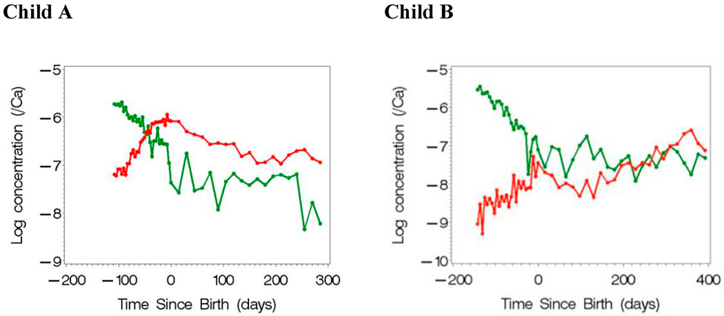
Prenatal and postnatal concentrations of Pb (red) and Mn (green) measured from two children’s teeth. (For interpretation of the references to color in this figure legend, the reader is referred to the Web version of this article.)

Data from children’s environmental health cohort studies offer the opportunity to evaluate critical windows of exposure. Distributed lagged regression models yield an estimate of the effect of exposure incurred at a specific time window while adjusting for exposures at earlier times, under the assumption that the effect of exposure varies smoothly over time. Our group was the first to propose using DLMs to uncover critical exposure windows for human health first by using air pollution data (Hsu et al., 2015; Wilson et al., 2017). Because the tooth biomarker has a similar temporally dense data structure to air pollution, we adapted this method to the tooth biomarker (Modabbernia et al., 2016). A limiting feature of DLMs is the requirement that all observations have complete data within the same time window. Exposure sampling times often vary across subjects and may be wide enough to mask important critical windows (e.g., trimesters of pregnancy). Thus, following previous work (Coull et al., 2014; Chen et al., 2015), we interchange roles of outcomes and exposures and use a functional spline model with time varying coefficients to evaluate associations between exposures and outcome:

$$X(t)={\beta }_0(t)+{\beta }_1(t)Y+\gamma z+u+\epsilon ,$$ (1)

where X(t) are standardized exposure concentrations over time, and Y is the standardized outcome variable, adjusted for covariates. The focus of the inference is the time-varying correlation between X and Y, depicted by β₁(t), with both Y and X centered and scaled. The random effect term, u, permits the assumption of a compound symmetry correlation pattern for intra-subject observations. Values of β₁(t) > 0 indicate higher concentrations are associated with higher mean outcome variable values, and vice versa. Time frames where Holms-Bonferroni-adjusted 95% confidence intervals on β₁(t) exclude 0 indicate critical windows of development.

Because of the growing interest in chemical mixtures research, Bello et al. (Bello et al., 2017) proposed a lagged version of WQS that uses an algorithm to extend the reverse DLM for analysis of mixtures. The rationale is based on the logic of WQS regression, where an empirically weighted index of standardized concentrations is constructed in multiple steps. The algorithm begins with equivalent weights for the initial WQS(t); estimates a reverse DLM on WQS(t); then, conditional on parameter estimates, improves the weights on WQS(t) from analysis of the residuals; then re-estimates the reverse DLM using the updated WQS weights. Confidence intervals are constructed on the time-varying association parameters. When the estimate of β₁(t) associated with WQS (t) is positive and significant, the mixture is positively correlated with the outcome; when the estimate is negative and significant, the mixture is negatively correlated and time-varying weights are graphically displayed.

An important feature in this algorithm is that it uses a reverse DLM which permits subjects to have measurements at different time points. For example, in Fig. 1, child A has Pb and Mn concentrations measured between 110 days before birth to roughly 300 days after birth. Child B has concentrations measured between 150 days before birth to almost 400 days after birth. The algorithm proposed by Bello et al. results in a temporal domain that includes the union of the time measurements across all subjects. A limitation of the algorithm, however, is the middle step where time varying weights are updated by simultaneously estimating a spline function per component in the mixture. When the number of components is small (say, 3 to 4) with a moderate to large sample size, the algorithm performs well in simulation studies. But, environmental exposure data often consists of more components; e.g., tooth data may have 15 metals and elements. Our objective herein is to extend lagged WQS regression to include temporally varying higherdimensional measures of exposure. We describe the revised approach in section 3 with an illustration in section 4. We conduct a sensitivity analysis on the algorithm through simulated data in section 5 with a final discussion in section 6.

3. Lagged WQS regression for mixtures with large numbers of components

WQS regression may be conducted using one of two ensemble steps where the final set of weights are averaged over the ensemble samples: i.e., (1) a bootstrap step whereby the ensemble step includes B (say, B = 100) bootstrap samples of subjects selected with replacement; or (2) a random subset step whereby subsets of components are selected randomly for analysis and averaged across all subsets (e.g., for analysis of 100 components, take 1000 random subsets of size 10). In the bootstrap ensemble step, the complex correlation pattern is at least roughly similar across all bootstrap samples; in the random subset version, the correlation pattern is broken apart for each subset thereby permitting a “de-correlation” of complex patterns in some of the analyses. We include these capabilities in a lagged version of WQS regression using the following steps for longitudinal exposures for multiple components that are each quantile scored (e.g., in deciles) across the temporal record.

Step 1:

Select a temporal domain and time unit (e.g., a week) for analysis. It is generally advisable, and for the bootstrap ensemble method essential, that the minimum number of subjects within any time unit in the domain exceeds the number of components in an ensemble step analysis plus the number of covariates. If a random subset ensemble procedure were used, it would be possible to construct a mixture wherein the number of mixture-components exceeds the number of subjects.

Step 2:

Conduct the first step of WQS regression (i.e., estimate the average weights from the ensemble step) within each time unit and output the estimated weights per time unit and the calculated weighted index per subject; i.e., WQS_i(t).

Step 3:

Estimate the time varying association across these indices using a reverse DLM model:

$$WQS(t)={\beta }_0(t)+{\beta }_1(t)Y+\gamma z+u+\epsilon$$ (2)

Step 4:

Plot the time varying association β₁(t) with corresponding confidence intervals. Plot smoothed functions of the estimated weights per component.

Since the focus of Step 2 is the estimation of the weights, and not hypothesis testing of the weighted index, there is no reason to split the data. Variations of the algorithm include estimating the mixture effect of the components by identifying the majority direction of the association across the bootstrap samples. Alternatively, the algorithm can be run by constraining the direction of the WQS regressions in a single direction, one at a time.

4. Illustration

Tooth biomarker concentrations were measured on 162 children from a pregnancy cohort. Fifteen elements (Ba, Bi, Cd, Co, Cr, Cu, Li, Mg, Mn, Mo, Ni, Pb, Sn, Sr, and Zn) were measured in both pre-natal and postnatal timepoints. Characteristics of the study participants included a population-centered neurological assessment scale, a sex indicator, maternal IQ, and a binary measure of socio-economic status (Table 1). Further details of the study data are not provided as the focus herein is on the biostatistical method and not on the particular neurological scale, resulting critical exposure windows, or the potential association with the measured elements.

Table 1.

Summary statistics for covariates with tooth biomarker data (N = 162).

Variable	Mean
% female	52%
Maternal IQ	86.3 (SD = 12.6)
% low SES	49%

The complex bi-variate correlation pattern among the metals across time includes both negative and positive Spearman correlation estimates with the strongest correlation estimates of 0.65 between Ba and Sr and 0.58 between Sr and Li (Fig. 2A). Interestingly, five of the elements (Bi, Cd, Co, Mo, and Ni) were measured near the limit of detection (LOD), and are included in the analyses as potential negative controls since their exposure concentrations may be somewhat random.

Fig. 2.

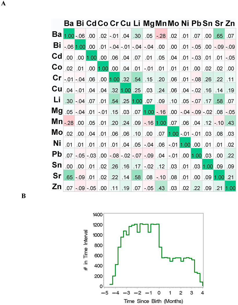
(A) Heat Map for Spearman correlation coefficients for all data (N = 162); and (B) histogram for the number of time points over time-since-birth (months).

Single element analyses were conducted for each of the 15 elements adjusted for covariates in Table 1 (Fig. 3). Positive associations were identified by a positive lower 95% Holms-Bonferroni confidence limit; negative associations would be identified by a negative upper 95% confidence limit. Here, concentrations of Ba are positively associated with Y, the neurological assessment score, postnatally; Sr is positively associated with Y at 2 months of age; and Zn is positively associated with Y in a prenatal time window. Significant windows of association were not identified for the other 12 elements.

Fig. 3.

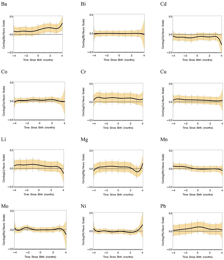
Single element reverse DLM analyses adjusted by covariates in Table 1 (n = 162 with an average of 136 time points per subject) with 95% Holm-Bonferroni simultaneous confidence intervals.

For analysis of the mixture of 15 elements, the lagged WQS regression was conducted over time in the following four steps.

STEP 1:

Concentrations for each of the elements measured over time were ranked into deciles. The unit for ‘time since birth’ (TSB) in the dataset is in months; i.e., TSB was calculated by dividing days by 30 with measurements taken roughly every 3rd or 4th day.

STEP 2:

Separate WQS regression analyses were conducted within quarter-month time units (i.e., rounding TSB into 0.25 intervals; Fig. 2B) between −4 months and 4 months where 0 is birth with a bootstrap ensemble step at each quarter-month. Final weights for the elements in each of the 32 analyses was the average over the time-specific 100 bootstrap samples (Fig. 4a.A with color legend in Fig. 4a.C). The number of bootstrap betas in the majority direction (Fig. 4a.B) indicate the strength of the signal in the majority direction. For example, the signal was almost always in the positive direction between 4 months before birth (i.e., TSB = −4) to birth; the signal is generally in the positive direction but with a decreased signal postnatally. The time-varying WQS(t) index was calculated for each subject using the estimated weights.

Fig. 4.

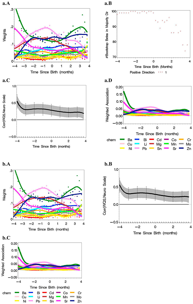
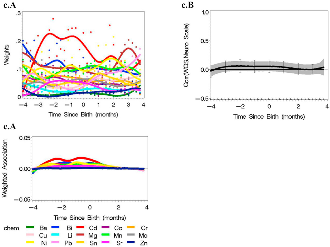
a Results from lagged WQS regression analysis of the mixture of 15 metals and a neuro scale unconstrained, adjusted by covariates in Table 1 (n = 162 with an average of 136 time points per subject). (A) WQS regression was conducted in quarter-month intervals with estimated weights and LOESS plot over analyses, and (B) the number of betas in the majority direction from the 100 bootstrap samples. (C) The resulting WQS(t) calculated in each quarter month analysis were used in a reverse DLM analysis with (D) related weighted association across the 15 metals plotted. b: Results from lagged WQS regression analysis of the mixture of 15 metals and a neuro scale constrained in the positive direction, adjusted by covariates in Table 1 (n = 162 with an average of 136 time points per subject). (A) WQS regression was conducted in quarter-month intervals with estimated weights and LOESS plot over analyses. (B) The resulting WQS(t) calculated in each quarter month analysis were used in a reverse DLM analysis with (C) related weighted association across the 15 metals plotted, c: Results from lagged WQS regression analysis of the mixture of 15 metals and a neuro scale constrained in the negative direction, adjusted by covariates in Table 1 (n = 162 with an average of 136 time points per subject). (A) WQS regression was conducted in quarter-month intervals with estimated weights and LOESS plot over analyses. (B) The resulting WQS (t) calculated in each quarter month analysis were used in a reverse DLM analysis with (C) related weighted association across the 15 metals plotted.

STEP 3:

A reverse DLM analysis was conducted on the association between Y and the estimated WQS(t) indices, adjusted for covariates in Table 1.

STEP 4:

The resulting association parameter with corresponding 95% confidence intervals were plotted (Fig. 4a.C). The weighted association (i.e., the estimated weights multiplied by the association parameter at each time point) for each of the 15 elements indicated a positive association both prenatally and postnatally. Ba and Sr were most highly weighted 4 months before birth with Pb, Mg and Zn more highly weighted within 2 months before birth. However, Ba, Zn and Pb dominated postnatally (Fig. 4D).

An alternative analysis strategy is to constrain the WQS indices over time to a single direction. This may be particularly helpful when the overall mixture includes both toxins and nutrients, for example, and it becomes essential to dissect discrete sub-mixtures. Here, the signal was primarily in the positive direction, so the resulting analysis with the beta constrained to be positive was essentially the same as the unconstrained analysis (Fig. 4b compared to Fig. 4a). In contrast, when the beta coefficient was constrained to be negative, there was no signal detected in the perinatal period (Fig. 4c).

5. Simulated data based on observed teeth data

The correlation pattern from the tooth data from a subset of seven element concentrations and covariates were used as the basis of the simulation study. Time (t) varying beta coefficients were assumed for each element in three different cases: Case 1: only X4 has a time-varying association; Case 2: X4, X5 and X7 have differing time-varying associations; Case 3: none of the variables are associated with the mean of Y. Specifically, as depicted in Fig. 5,

Fig. 5.

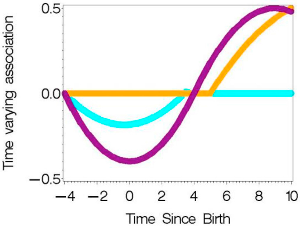
Assumed time varying association between Y and X4 (purple: Cases 1,2), X5 (orange: Case 2), and X7 (cyan: Case 2) in simulated data. (For interpretation of the references to color in this figure legend, the reader is referred to the Web version of this article.)

Cases 1,2:

$$\begin{gathered} {\beta }_4=(t-4)\{-0.2(t+4)+0.025{(t+4)}^2\} \\ +(t\ge 4)\{0.2(t-4)-0.02{(t-4)}^2\} \end{gathered}$$

Case 2:

$$\begin{gathered} {\beta }_5=(t>5)\{0.15(t-5)-0.01{(t-5)}^2\} \\ {\beta }_7==(t<4)\{-0.1(t+4)+0.0135{(t+4)}^2\} \end{gathered}$$

In Case 3, all beta coefficients were set to 0. The simulated Y values were assumed to be normally distributed, with mean mu which is linear in the Xs with time-varying regression coefficients; i.e., $\mu ={\Sigma }_{j=1}^7{\beta }_j{X}_j$ It is important to consider the change in sample sizes over time where the 3 months prior to birth have roughly 240 measurements; the first 4 months after birth has roughly 130 measurements; and 4–10 months of age has only about 50 measurements per time interval (Fig. 2B).

The new version of lagged WQS was conducted in the following steps. All concentrations were ranked into deciles for each element. WQS regression was conducted in quarter month intervals with the weights and WQS(t) combined across analyses. The reverse DLM model of WQS(t), as given in equation (2), was estimated adjusted for the covariates. Estimates of the correlation between WQS and Y were plotted with 95% family-wise Holm-Bonferroni confidence intervals for all three cases (Fig. 6).

Fig. 6.

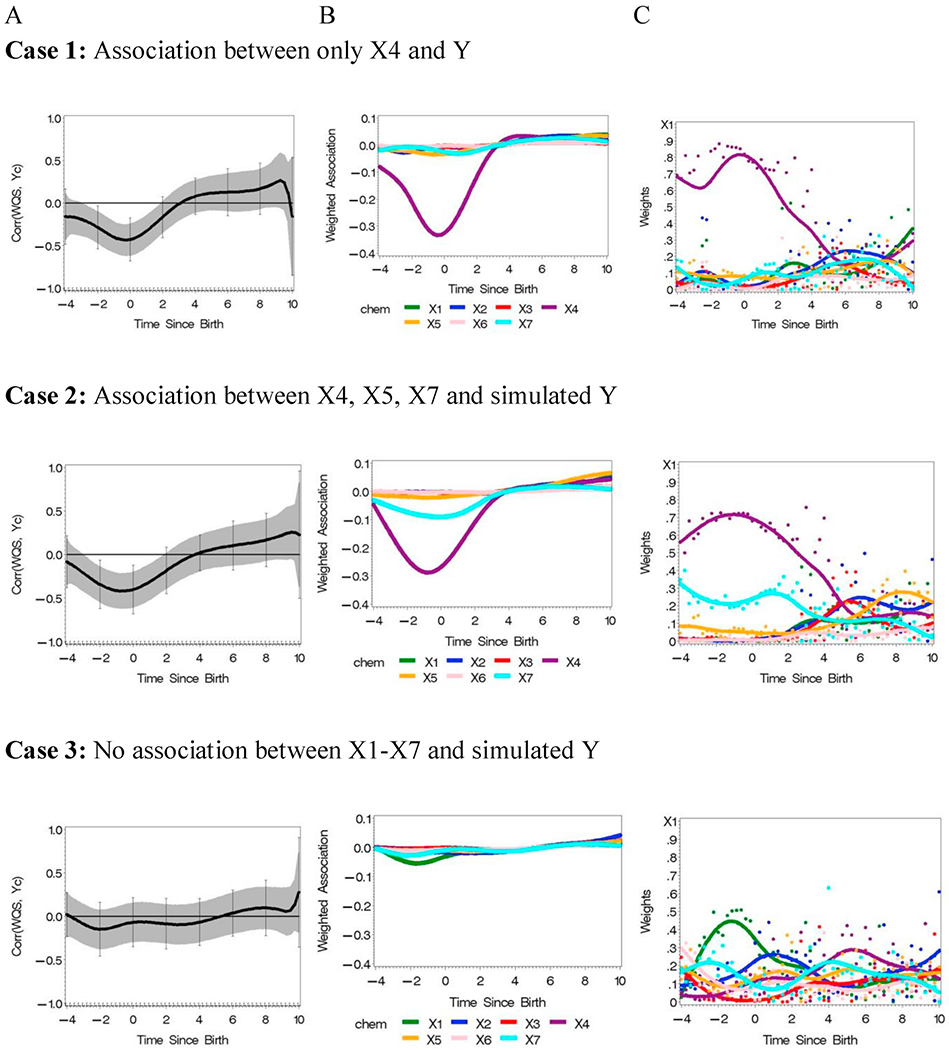
Analysis of simulated data from three cases using observed teeth data (N = 138) with hypothetical associations with an outcome variable Y.

In Case 1, a peri-natal negative association was detected between 2 months before birth and 1 month after birth. Only X4 was associated with the association as evident in Fig. 6, Case 1B,C). The weights from the WQS regressions as depicted by the dots in Figure C demonstrate the association with the largest sample size provide the strongest signal; the smaller sample size after about 4 months was not large enough to estimate the postnatal positive association. Further, the decrease in sample size was also evident in the increase in variability of adjacent WQS weights as depicted, for example, for X4 in Fig. 6C Case 1.

In Case 2, the strongest peri-natal significant association was with X4 but a negative association was also detected for X7. Again, the sample size was too small to detect the association after about 4 months for X5 and X4. And, again, the variability of adjacent WQS weights increased in this later time frame, for example, for X4 in Fig. 6C Case 2. Finally, there was no evidence of an association with any of the components in Case 3, which was as designed.

6. Discussion

We have presented a revised version of lagged WQS regression that may be operationally generalizable to combinations of many chemicals. The original algorithm proposed in Bello et al. (Bello et al., 2017) fit separate splines to estimated weights of components over time, which worked well for 3 or 4 components but was untenable for dozens of components due to the number of required parameters. Herein, we propose to compromise the flexibility of the full time-domain in the design across subjects by selecting a somewhat narrower time domain and conduct WQS regression in time-specific analyses. We demonstrate the approach using quarter-month analyses between 4 months before birth to 4 months after birth. The advantage is that the time-specific analyses may utilize both the bootstrap (Carrico et al., 2015) and the random subset (Curtin et al., 2019) versions of the ensemble step in WQS regression.

The time-specific WQS regression analyses result in local estimates of weights that are more precise for larger sample sizes. In the simulation study conducted herein, the specified associations were detected in time intervals with sample sizes that exceeded about 100 measurements. For smaller sample sizes, the weights were associated with more variability and the simulated signals were not detected.

The proposed revised lagged WQS regression model allows the inference to be focused in both directions throughout the observed time frame by constraining in each direction one at a time – as demonstrated in Fig. 4b and c. This may be particularly useful as the number of components increases and the mixtures include both toxins and nutrients – or more generally, where components are positively or negatively associated with the outcome. Such a case was observed in an analysis of the association between PCB exposures and time-to-pregnancy (Gennings et al., 2013); the WQS indices were significantly associated with the time to pregnancy in both directions. The components with non-negligible weights in the positive direction were distinct from the components with weights in the negative direction. The proposed lagged WQS regression model allows for such associations to change over time.

We have used a truncated power function spline in our analyses for both β₀(t) and β₁(t) using PROC NLMIXED in SAS. (The SAS code is available in the supplementary material.) For general model selection criteria that may include different spline functions and covariates, there is a literature that considers temporal dependencies with flexible spline functions and selection criteria on the basis of profile likelihood (Hauptmann et al., 2001), AIC (Hauptmann et al., 2000; Hauptmann et al., 2002; Berhane et al., 2008), and BIC (Sylvestre and Abrahamowicz, 2009).

Finally, there are some limitations in using DLMs and tooth biomarkers that should be acknowledged. We suggest using the square root of the number of components in the random-subset ensemble step, but we have not fully characterized the sensitivity of the results to this choice. Perhaps model selection criteria (e.g., AIC, BIC) may be useful in further characterizing the size of the subsets. There are well known seasonal aspects to environmental exposures (e.g., lead tends to increase in summer months perhaps due to seasonal differences in Vitamin D metabolism (Kemp et al., 2007)). However, analysis of the tooth in TSB units, instead of calendar units, homogenizes these seasonal effects. As previously noted, some elements are nutritional (zinc, manganese, copper among others) even though they may be toxic at high exposure levels, while other elements are only toxins (lead, tin) but may have critical exposure windows. Reverse DLMs are models of time-varying association for either single chemicals or mixtures that are either positive or negative at a given point in time. This allows for the detection of differential effects, essentially comprising sub-mixtures of components within the overall mixture, which associate either positively or negatively with health endpoints. There are also differences in detection limits and precision for chemicals measured concurrently in teeth. It is possible that not all chemicals deposit in teeth or that they deposit in a way that doesn’t reflect body burden. Either way, we use quantile scores for measurements over time for each component. Nonetheless the ability to measure environmental exposures in short time intervals has great promise in improving our understanding of environmental influences on human health and the role of exposure timing in determining toxicant effects.

Understanding the role of exposure timing in driving human health effects is an important area of study that can address issues such as the optimal timing for prevention interventions. If an environmental factor predicts a health outcome only during a critical exposure window, public health efforts to reduce the prevalence of disease can focus on this window with maximal benefit and potentially reduced costs. For example, if a chemical predicts later onset of autism when exposure occurs in the 3rd trimester but not post-natally, then public health interventions can be directed at the 3rd trimester. A converging issue in public health research is how to study the joint impact of multiple exposure - both positive such as good nutrition and toxic, such as environmental neurotoxins. In this paper we merge these two issues and illustrate methodologies that can jointly address both. A key advantage in this approach is that the weights estimated in the lagged WQS can also allow public health clinicians and policy makers to prioritize both the timing of intervention and identify the mixture components that are most important to address. While further work is needed to replicate results, and to refine these methods and expand the chemical measures available from exposure biomarkers such as the tooth, there is great promise in our ability to address all of these issues in future studies.

References

- Arora M, Austin C, 2013. Teeth as a biomarker of past chemical exposure. Curr. Opin. Pediatr 25 (2), 261–267. [DOI] [PubMed] [Google Scholar]
- Arora M, Austin C, Sarrafpour B, Hernandez-Avila M, Hu H, Wright RO, Tellez-Rojo MM, 2014. Determining prenatal, early childhood and cumulative long-term lead exposure using micro-spatial deciduous dentine levels. PloS One 9 (5), e97805. [DOI] [PMC free article] [PubMed] [Google Scholar]
- Bello GA, Arora M, Austin C, Horton MK, Wright RO, Gennings C, 2017. Extending the Distributed Lag Model framework to handle chemical mixtures. Environ. Res 156, 253–264. [DOI] [PMC free article] [PubMed] [Google Scholar]
- Berhane K, Hauptmann M, Langholz B, 2008. Using tensor product splines in modeling exposure-time-response relationships: application to the Colorado Plateau Uranium Miners cohort. Stat. Med 27 (26), 5484–5496. [DOI] [PMC free article] [PubMed] [Google Scholar]
- Carrico C, Gennings C, Wheeler DC, Factor-Litvak P, 2015. Characterization of weighted quantile sum regression for highly correlated data in a risk analysis setting. J. Agric. Biol. Environ. Stat 20 (1), 100–120. [DOI] [PMC free article] [PubMed] [Google Scholar]
- Chen YH, Ferguson KK, Meeker JD, McElrath TF, Mukherjee B, 2015. Statistical methods for modeling repeated measures of maternal environmental exposure biomarkers during pregnancy in association with preterm birth. Environ. Health 14, 9. [DOI] [PMC free article] [PubMed] [Google Scholar]
- Coull B, Claus Henn B, Wright RO, Arora M, 2014. Statistical methods for analyzing critical windows of metal exposures using the tooth biomarker. In: 2014 Conference of the International Society of Exposure Science. Cincinnati, OH. [Google Scholar]
- Curtin P, Kellogg JJ, Cech NB, Gennings C, 2019. A random subset implementation of weighted quantile sum (WQSRS) regression for analysis of high-dimensional mixtures. Communications in Statistics - Simulation and Computation. Taylor & Francis; Onlinehttps://doi.org/l0.1080/03610918.2019.1577971. [Google Scholar]
- Czarnota J, Gennings C, Wheeler DC, 2015. Assessment of weighted quantile sum regression for modeling chemical mixtures and cancer risk. Cane. Inf 14 (Suppl. 2), 159–171. [DOI] [PMC free article] [PubMed] [Google Scholar]
- Gennings C, Carrico C, Factor-Litvak P, Krigbaum N, Cirillo PM, Cohn BA, 2013. A cohort study evaluation of maternal PCB exposure related to time to pregnancy in daughters. Environ. Health 12 (1), 66. [DOI] [PMC free article] [PubMed] [Google Scholar]
- Hauptmann M, Berhane K, Langholz B, Lubin J, 2001. Using splines to analyse latency in the Colorado Plateau uranium miners cohort. J. Epidemiol. Biostat 6 (6), 417–424. [DOI] [PubMed] [Google Scholar]
- Hauptmann M, Pohlabeln H, Lubin JH, Jockel KH, Ahrens W, Bruske-Hohlfeld I, Wichmann H, 2002. The exposure-time-response relationship between occupational asbestos exposure and lung cancer in two German case-control studies. Am. J. Ind. Med 41 (2), 89–97. [DOI] [PubMed] [Google Scholar]
- Hauptmann M, Wellmann J, Lubin J, Rosenberg P, Kreienbrock L, 2000. Analysis of exposure-time-response relationships using a spline weight function. Biometrics 56, 1105–1108. [DOI] [PubMed] [Google Scholar]
- Hsu HH, Chiu YH, Coull BA, Kloog I, Schwartz J, Lee A, Wright RO, Wright RJ, 2015. Prenatal particulate air pollution and asthma onset in urban children. Identifying sensitive windows and sex differences. Am. J. Respir. Crit. Care Med 192 (9), 1052–1059. [DOI] [PMC free article] [PubMed] [Google Scholar]
- Kemp FW, Neti PV, Howell RW, Wenger P, Louria DB, Bogden JD, 2007. Elevated blood lead concentrations and vitamin D deficiency in winter and summer in young urban children. Environ. Health Perspect 115 (4), 630–635. [DOI] [PMC free article] [PubMed] [Google Scholar]
- Modabbernia A, Velthorst E, Gennings C, De Haan L, Austin C, Sutterland A, Mollon J, Frangou S, Wright R, Arora M, Reichenberg A, 2016. Early-life metal exposure and schizophrenia: a proof-of-concept study using novel tooth-matrix biomarkers. Eur. Psychiatr 36, 1–6. [DOI] [PMC free article] [PubMed] [Google Scholar]
- Neter J, Kutner M, Nachtsheim C, Wasserman W, 1996. Applied Linear Statistical Models, fourth ed. (Chicago, Irwin: ). [Google Scholar]
- Orton F, Ermler S, Kugathas S, Rosivatz E, Scholze M, Kortenkamp A, 2014. Mixture effects at very low doses with combinations of anti-androgenic pesticides, antioxidants, industrial pollutant and chemicals used in personal care products. Toxicol. Appl. Pharmacol 278 (3), 201–208. [DOI] [PubMed] [Google Scholar]
- Sylvestre M-P, Abrahamowicz M, 2009. Flexible modeling of the cumulative effects of time-dependent exposures on the hazard. Stat. Med 28, 3437–3453. [DOI] [PubMed] [Google Scholar]
- Tu YK, Gunnell D, Gilthorpe MS, 2008. Simpson’s Paradox, Lord’s Paradox, and Suppression Effects are the same phenomenon-the reversal paradox. Emerg. Themes Epidemiol 5, 2. [DOI] [PMC free article] [PubMed] [Google Scholar]
- Wilson A, Chiu YM, Hsu HL, Wright RO, Wright RJ, Coull BA, 2017. Potential for bias when estimating critical windows for air pollution in children’s health. Am. J. Epidemiol 186 (11), 1281–1289. [DOI] [PMC free article] [PubMed] [Google Scholar]
Associated Data
This section collects any data citations, data availability statements, or supplementary materials included in this article.